Multimodal Deep Learning for Participatory Public Art Assessment: Integrating Computer Vision and Behavioral Analytics for Community Engagement

Resumen

This paper presents a new multimodal deep learning architecture for evaluating public engagement with public art. With the help of 3D convolutional neural networks and cross-attention transformers, the proposed model extracts spatio-temporal information and interactions, thereby outperforming other methods in predicting engagement, recognizing emotions, and assessing aesthetics.

Resumen

In this work, a deep learning-based multimodal framework for evaluating public engagement with public art is introduced by combining computer vision and behavioral analysis. Existing multimodal models have primarily been applied in domains such as educational settings and behavior analysis, while their application to public art assessment remains limited by challenges in representing subjective human factors, complex behaviors, and interactions across modalities. To address these challenges, the proposed framework employs a Transformer-based architecture to integrate multimodal information and model cross-modal interactions. Image and video inputs representing artworks and participant behaviors, including movement, gaze, and interaction, are processed using 3D convolutional neural networks to extract spatiotemporal features, followed by modality-specific encoding and adaptive fusion using cross-attention. The framework generates outputs related to engagement, emotion recognition, and interaction assessment. For component-level evaluation before real-world public art deployment, the framework was evaluated on three complementary benchmark datasets: NTU RGB+D, Kinetics-700, and AVA (Aesthetic Visual Analysis), representing behavioral, activity recognition, and aesthetic perception tasks. In the classification task, the accuracy obtained was 92.0% and the F1-score of 0.909 for NTU RGB+D, while that of Kinetics-700 was 89.0% and the F1-score of 0.878. The AVA dataset was evaluated using aesthetic-score regression, yielding a Pearson correlation coefficient of 0.87. These findings provide component-level evidence of computational effectiveness but do not constitute end-to-end validation in real-world public art settings.

Introducción

The value of art education has become increasingly apparent in today's academic landscape. It has a significant effect on children's overall growth and encourages their artistic and creative skills. Personalized instruction has emerged as a major trend in the advancement of art instruction as educational philosophies continue to change¹. Some students experience low excitement and poor learning outcomes as a result of the conventional "one-size-fits-all" education model's inability to address these unique requirements². The collection of behavioral information from multiple perspectives during the art learning process is now possible thanks to the development of multimodal data-gathering and analysis methodologies³. These data demonstrate notable technological advantages for analyzing art-learning behaviors and provide evidence for a better understanding of learners' behavioral patterns⁴.

Convolutional and recurrent neural networks have demonstrated effectiveness in applications such as autonomous systems, audio processing, and image recognition⁵. As a result of this integration, smart, adaptive systems that can react dynamically to inputs in real time have been developed. Internet of things (IoT)-enhanced artworks, in contrast to conventional static forms, can leverage motion, sound, and visual data to enable dynamic, adaptable interactions. As a result, the distinction between the viewer and the artwork has become increasingly blurred in kinetic, algorithmic, biosensor-based, and interactive art forms^6,7.

Increased computing power, large-scale annotated datasets, and advances in deep learning have enabled complex representation learning^8,9. Deep learning is increasingly applied in creative industries, including the use of Generative Adversarial Networks (GANs) to generate realistic media content^10,11.

In sports, artistic performances, and similar contexts, action recognition is also crucial¹². In sports, analyzing athletes’ postural movements and comparing them with reference movement patterns can help identify performance deficiencies and guide training. Similarly, in performance arts such as dance, movement analysis can support technique assessment and improve training effectiveness. Additionally, human motion recognition can help performers complete their performances and training more effectively through motion analysis¹³. Feature extraction and classification are key components of human action-recognition systems¹⁴.

Recent research on multimodal deep learning has demonstrated success in areas such as art education, human activity recognition, and behavior analysis. For example, previous studies have emphasized the integration of multimodal features to analyze behavior in art education and to support personalized teaching. However, research on multimodal deep learning has mainly focused on improvements in cross-modal integration and representation learning^15,16. In addition, human activity recognition studies use predefined datasets rather than addressing the challenges posed by public environments.

A further research gap is the lack of a unified methodology that integrates computer vision and behavioral analytics to comprehensively assess human interactions with public artworks. Dataset availability also remains limited, particularly for real-world scenarios involving community engagement, public art, and environmental conditions^17,18. In addition, existing models often provide limited interpretability regarding the factors associated with audience engagement.

A generative adversarial network (GAN)-based pencil-drawing learning system was developed to support art education¹⁹. Previous studies have also analyzed student assignments to characterize learning progress, preferred styles, and individual learning needs^20,21, with the aim of supporting personalized and collaborative art education^22,23. Emerging technologies, including 5G and virtual reality, can enhance interactive artistic experiences by enabling communication, immersive content, and audience participation²⁴.

Recent studies have demonstrated that generative AI has been applied across diverse creative domains, including graphic design, architecture, fashion, and visual content generation. These studies highlight the ability of deep learning models to support creative workflows and generate novel visual content. However, relatively few studies have explored multimodal deep learning frameworks for assessing human engagement with participatory public art, particularly by integrating visual, behavioral, and contextual information²⁵. When generative art was applied to architecture, the author found that it produced nearly limitless structural variations and more creative work²⁶. Previous research has also explored the integration of generative and futuristic art to investigate new aesthetic components and procedural approaches²⁷. The author also discusses how computational art can assess fashion designs and generate original concepts based on form analysis of earlier designs²⁸. Other researchers have examined how generative AI may affect visual content advertising²⁹. VQGAN and CLIP together give designers greater adaptability and creative control over the design process by enabling them to produce unique graphics based on textual clues³⁰. Because deep learning models like VQGAN and CLIP can instantaneously present a wide variety of visual alternatives based on textual ideas, they allow designers to work more quickly and effectively³¹.

Gao et al.³² proposed a multimodal dance emotion recognition framework using MobileNetV2 with a lightweight attention module to enhance salient feature learning. The model jointly processes channel and spatial information while employing 1 x 1 and 3 x 3 convolutions to reduce computational complexity. Separate audio, video, and multimodal fusion networks were developed to achieve effective deep feature learning. Teng et al.³³ introduced a sports action recognition framework based on adaptive graph convolution and neural tensor networks (NTN). The model constructs a global adjacency matrix using an attention mechanism and NTN, dynamically updates neighboring nodes through the TopK strategy, and extracts temporal and contextual information using hybrid pooling to improve motion representation by jointly modeling joint, bone, and movement features. Yin et al.³⁴ presented an anomaly detection method for the 6G Internet of Everything (IoE) that uses a deep autoencoder and a capsule graph convolutional network, optimized with the Sparrow Search Algorithm. The framework generates pseudo-abnormal samples, performs capsule-based dynamic feature fusion, reconstructs bottleneck features to maximize anomaly discrimination, and optimizes network parameters using the Sparrow Search Algorithm. Chen³⁵ developed a multimodal music emotion recognition framework based on a dual-channel Long Short-Term Memory (LSTM) that models auditory and visual information separately. The extracted features are fused using the Analytic Hierarchy Process (AHP) at the decision level, thereby improving emotion recognition accuracy while reducing training time. Given the limited availability of real-world public art datasets, a proof-of-concept framework requires evaluation on complementary benchmark datasets that can serve as surrogate sources to validate its individual computational components before deployment in actual public art environments.

The aim of this study was to develop a multimodal, deep learning-based proof-of-concept framework to assess public engagement with participatory public art using computer vision and behavioral analytics. Specifically, the framework integrates visual, behavioral, and contextual information to estimate engagement, emotion, and interaction-related outcomes. Because suitable real-world public art datasets are limited, benchmark datasets are used as surrogates for component-level training and evaluation. The performance of the proposed framework is subsequently compared with representative baseline models to assess its computational effectiveness.

The main contributions of this study are as follows: (1) A multimodal proof-of-concept framework that integrates computer vision and behavioral analytics is proposed to assess public engagement with participatory public art, bridging the gap between computational analysis and community participation. (2) An encoder-decoder-based multimodal fusion approach incorporating cross-attention is introduced to model relationships among visual, behavioral, and contextual information and enhance feature representation. (3) A unified processing framework is presented to integrate heterogeneous data through spatiotemporal feature extraction using 3D CNNs and modality-specific encoding. (4) A community-oriented evaluation system is developed to assess public art performance using behavioral outcomes, including engagement scores, emotion recognition, and interaction levels. (5) The proposed framework is evaluated using the NTU RGB+D, Kinetics-700, and AVA benchmark datasets, providing component-level evidence of its activity, behavioral, and aesthetic assessment capabilities. (6) Behavioral analytics and attention mechanisms are incorporated to characterize the contribution of different modalities to engagement and interaction assessment.

While a number of multimodal deep learning techniques have been proposed for applications such as cross-media understanding, human activity recognition, art education, and behavioral analysis, their goals, fusion strategies, and application domains differ markedly from the proposed framework for participatory public art assessment. Table 1 compares representative techniques across input modalities, fusion mechanisms, behavioral analytics capabilities, application domains, and major limitations to position the proposed study relative to previous studies. Although these methods employ multimodal learning, they do not simultaneously integrate visual, skeletal, auditory, and contextual information for participatory assessment of public art. Additionally, most current research does not integrate behavioral analytics, engagement prediction, and aesthetic evaluation into a single framework. By integrating behavioral analytics, Transformer-based multimodal fusion, and cross-modal attention into a single end-to-end framework specifically designed for public art appraisal, the proposed architecture addresses these limitations.

Protocolo

This study did not involve human participants. All data were utilized in accordance with applicable usage policies; therefore, ethical approval and consent to participate were not required.

The proposed framework integrates multimodal visual, behavioral, and contextual data to assess participatory public art. Following data acquisition and preprocessing, spatiotemporal features are extracted using a pretrained 3D CNN and encoded into modality-specific representations. A cross-attention Transformer fuses these representations to generate a unified feature embedding, which a behavioral analytics module then analyzes to estimate engagement, interaction, and aesthetic perception. The overall workflow of the proposed framework is illustrated in Figure 1.

Step 1: Dataset acquisition and preparation

To begin with, the NTU RGB+D, Kinetics-700, and AVA datasets were extracted from their respective databases and preprocessed individually using their original annotations and identifiers. Each of the three datasets was divided into training, validation, and testing sub-datasets, in the ratios of 70%, 15%, and 15%, respectively. Identifiers for each individual dataset were used during the division process to ensure that no subject, source video, or sample would appear in both the training and independent testing sub-datasets.

Step 2: Multimodal data preprocessing

Multimodal data were processed using Gaussian filtering to eliminate noise, normalization to ensure feature consistency, uniform frame sampling, and data augmentation to improve model robustness. As a result, standardized multimodal data were obtained and used for the feature extraction stage.

Step 3: Multimodal feature extraction

The encoding of the input modalities was based on their intrinsic native data representation in their respective datasets. In the case of NTU RGB+D, the RGB, depth, and skeleton sequences were individually encoded to extract modality-specific features. Similarly, for Kinetics-700, the video frames and the associated audio sequence were encoded separately. However, in the case of AVA, the image was extracted using the visual feature extractor, while the associated aesthetic score remained the ground-truth label for that image.

Step 4: Feature embedding and alignment

These features were mapped into a shared 256-dimensional latent embedding space by utilizing linear projection layers. The projection was performed separately for each modality present in any dataset. The alignments between modalities belonging to the same sample were performed using their natural temporal alignment or the sample itself. No cross-dataset pairing or concatenation was done. In case where multiple synchronized modalities were present, the aligned embeddings were then passed through the cross-modal attention layer.

Step 5: Cross-modal attention-based fusion

The cross-modal attention Transformer was employed with embeddings from each modality in each dataset. In the case of NTU RGB+D, the cross-attention learned interactions among the embeddings of the RGB, depth, and skeleton modalities. In the case of Kinetics-700, the cross-attention learned interactions between the video and audio modalities. In the case of AVA, where image data along with the aesthetic rating are provided but no behavioral or audio input is available, there was no need for cross-modal attention, and the image representation was fed directly to the prediction head.

Step 6: Model training

The above multimodal aspects were used to train the Behavioral Analytics model with the AdamW optimizer and the Cross-Entropy and Contrastive Loss functions. The model was trained over 10 epochs with a batch size of 32 and a learning rate of 0.001. These same training and optimization parameters were used for the five experiments.

Step 7: Validation and optimization

Validation of the model was performed after each of 10 training epochs. The checkpoint with the highest validation accuracy across the 10 training epochs was selected as the best model for testing on the test set.

Step 8: Performance evaluation

The performance of the optimized model was assessed on the independent test set. Performance was evaluated using accuracy, precision, recall, F1-score, mean squared error (MSE), mean absolute error (MAE), Pearson correlation coefficient (PCC), and engagement score.

The accuracy, precision, recall, and F1 score of the classification tests on NTU RGB+D and Kinetics-700 were derived from predictions on the separate test sets. Accuracy is computed as the ratio of correct classifications to the total number of samples, while precision and recall are derived using the counts of true positives, false negatives, and false positives. The F1 score is computed as the harmonic mean of precision and recall. Classification scores are derived separately for each dataset and were not aggregated between NTU RGB+D and Kinetics-700.

Validation checkpoints and intermediate outputs

To ensure reproducibility of the suggested pipeline, the intermediate outputs were validated at the end of each step. Once data processing was complete, samples were visually analyzed to validate the frame-extraction procedure, which included Gaussian filtering, normalization, and temporal synchronization across all modalities. During the feature extraction stage, the feature dimensions were verified to be consistent with the multimodal transformer. The consistency of the embeddings and attention weights was analyzed after the feature alignment and cross-modal fusion steps to validate the modality fusion process. During training, validation accuracy and loss were calculated at the end of each epoch, and the model with the highest validation accuracy was saved as the final checkpoint.

Data acquisition

For behavioral analysis, human activity modeling, and aesthetic perception assessment, NTU RGB+D³⁶, Kinetics-700³⁷, and AVA³⁸ were used, respectively. The features of the datasets are summarized in Table 2. For the proposed methodology, the following three benchmark datasets covering different types of data were chosen: (1) NTU RGB+D, which consists of more than 56,000 video sequences with 60 activities performed by 40 subjects, 4 million frames with 3D skeletal data (with 25 joints per frame); (2) Kinetics-700, which includes 650,000 audiovisual clips corresponding to 700 human actions classes, each video having on average 10 s duration; and (3) AVA, comprising approximately 255,000 images with crowdsourced aesthetic ratings on a scale of 1–10.

NTU RGB+D, Kinetics-700, and AVA were deliberately chosen because they collectively capture the primary modalities required by the proposed framework, even though they were not initially intended for interactive public art assessment. For modeling participant movements and interaction behaviors, NTU RGB+D offers synchronized RGB, depth, and skeleton data. While AVA offers crowdsourced aesthetic ratings that enable assessment of perceptual responses, Kinetics-700 provides extensive, unrestricted human activity recordings that capture a variety of real-world behavioral contexts. These datasets served as complementary benchmarks for component-level validation of the proposed architecture before evaluation in real-world public art settings. It is important to note that the datasets were used independently as benchmarking sources and not combined as samples; thus, multimodal correspondence was achieved only for modalities within the same sample of a given dataset.

Data preparation and preprocessing

The NTU RGB+D (NTU RGB+D 60), Kinetics-700, and AVA datasets were obtained from their respective repositories and validated to ensure data integrity before preprocessing. Each dataset was preprocessed separately, using the original annotations and metadata, without mixing samples across datasets.

Data splitting and leakage prevention

Each dataset was split into training, validation, and test sets in the proportions 70%, 15%, and 15%, respectively. The splitting process was performed prior to model training and was repeated across all experiments. In the case of NTU RGB+D, the splitting unit was chosen based on the available unique identifiers so that samples corresponding to the same identifier are never present in both the training and test splits. In the case of Kinetics-700, samples from the same source video were kept in the same split to avoid source-video overlap between training and test samples. For the AVA, the dataset samples were split by their original identifiers, removing any duplicates or overlaps. The training split was used to train the model; the validation split was used for model selection and monitoring of convergence; and the test split was held out and never accessed prior to the evaluation phase. Therefore, none of the subjects or source samples used for training were included in the independent test split.

Dataset-specific multimodal sample construction and fusion

Multimodal samples were generated separately for each benchmark dataset and did not involve combining samples from NTU RGB+D, Kinetics-700, and AVA. In NTU RGB+D, each sample was represented as an action sequence consisting of RGB, depth, and skeleton streams of one subject performing a particular action at a certain point in time. Alignment between RGB and depth frames was performed using their common frame index, and alignment between skeleton joint coordinates and action time was also performed. Three different representations were independently encoded and then mapped into a common 256-dimensional embedding space for cross-modal attention.

In Kinetics-700, each sample consisted of an audiovisual clip, with the video frames serving as the visual representation and the audio clip as the contextual representation. Temporal alignment between the video and audio streams, based on their timestamps, was performed prior to encoding and projection into a common embedding space, followed by cross-modal attention.

In AVA, each instance consisted of an image with its crowdsourced aesthetic score. The image was used as the input for aesthetic-score regression, whereas the aesthetic score served as the prediction target and was not treated as an input modality. Because AVA does not contain synchronized behavioral or audio streams, its primary regression evaluation was performed using the available visual information. Additional architecture-level diagnostic analyses were also performed to compare the behavior of the evaluated model configurations. These diagnostic measures were used for model comparison and do not indicate that AVA contains native behavioral or temporal modalities.

In light of the above information, the proposed cross-modal Transformer operates on the modalities available in the dataset rather than requiring all three modalities in every instance. In cases where multiple modalities are available, the corresponding modality-specific embeddings are projected into the latent space, and cross-attention is applied across them. If only one modality is available as input, the corresponding encoded representation skips cross-modality attention and goes directly to the prediction head. Therefore, the benchmark data sets provide component-level evaluation of the proposed multimodal architecture, in contrast to a combined evaluation across data sets.

NTU RGB+D, Kinetics-700, and AVA were not treated as multimodal behavior datasets in the same way; they were considered distinct datasets to evaluate components separately. NTU RGB+D and Kinetics-700 were used for behavior evaluation on temporally structured data, while AVA was used for evaluation on static images with crowd aesthetic scoring. For this reason, temporal behavior evaluation measures such as attention time, interaction, and social participation were assessed using the NTU RGB+D and Kinetics-700 datasets.

Frame extraction for video

Video frames were sampled at regular intervals to reduce redundancy while preserving motion information for spatiotemporal feature learning. Equations (1)–(16) were adapted from previously published formulations³².

F_t=V(t.∆t),    t=1,2,3,…….,N  (1)

Here, F_t indicates the frame that has been sampled at the time step t and ∆t indicates the interval between frames. To ensure consistency across different lengths of video clips, an equal number of frames N per clip was chosen based on uniform sampling as follows:

   (2)

Here T denotes the clip duration. Uniform sampling reduced computational redundancy while preserving motion information for downstream feature extraction.

Noise removal for audio/behavior signals

Gaussian filtering was applied to audio and behavioral signals to reduce sensor noise, interference, and other high-frequency artifacts, as follows:

  (3)

In the above equation,  is the signal to be smoothed, and  w(i) represents Gaussian weights. This filtering reduced high-frequency noise in the signals.

Data alignment across modalities

Because the modalities were acquired at different sampling rates, temporal alignment was required. Temporal alignment was performed using interpolation as follows:

   (4)

where f_m denotes the sampling rate of the modality m and f_ref denotes the reference frequency. Moreover, for feature-level alignment of data captured using various modalities, each modality was mapped onto a latent space, represented by:

Z_m= Φ_m (X_m)  (5)

where Φ_m represents the encoder for the respective modality.

Data augmentation for generalization

Augmentation was performed to increase robustness and avoid overfitting. Transformations like rotation, scaling, and flipping were applied to images:

I'=T(I;θ)  (6)

where T denotes the transformation operation and θ is a parameter set. This helped to account for different views and lighting conditions. Augmentation strategies such as time warping and jittering were applied for temporal and behavioral data:

x'(t) = x(t+δ,δ~N(0,σ²))  (7)

where δ adds randomness to the data.

Algorithm 1: multimodal data preprocessing

Input: D_v is video data (NTU RGB+D, Kinetics-700), D_b is behavioral data (skeleton, gaze), D_a is audio/context data

Output: D_processed is pre-processed multimodal dataset

Begin

Step 1: Initialize D_processed = ∅

Step 2: For each sample i in the dataset do

Step 3: Frame extraction

Step 4: Extract frames F_i from video D_v(i) at interval ∆t

Step 5: Noise removal

Step 6: Apply filtering on behavioral data:

D_{b_clean} =Filter(D_b (i))

Step 7: Apply smoothing on audio data:

D_{a_clean} = Smooth(D_a (i))

Step 8: Normalization

Step 9: Normalize all modalities:

F_{i_norm} = normalize(F_i)

D_{b_norm} = normalize(D_{b_clean})

D_{a_norm} = normalize(D_{a_clean})

Step 10: Dataset-specific modality alignment

Step 11: Align modalities temporally:

[F_{i_align},D_{b_align},D_{a_align}]=Align([F_{i_norm},D_{b_norm},D_anorm))

Step 12: Data augmentation

Step 13: Apply transformations:

F_{i_aug} = Augment([F_{i_align})

D_{b_aug} = Augment([D_{b_align})

Step 14: Construct dataset-specific multimodal representation

Step 15: D_processed = D_processed U {F_{i_aug},D_{b_aug},D_{a_align}}

Step 16: End For

Step 17: Return  D_processed 

End

Algorithm 1 provided a systematic preprocessing procedure before model training. First, relevant video frames were extracted from the datasets at uniform intervals to maintain temporal consistency. Behavioral and audio signals were then filtered and smoothed to reduce noise and improve signal quality. All modalities were subsequently normalized to ensure consistent feature distributions. Temporal alignment was performed to synchronize the video frames with the corresponding behavioral and audio signals. Finally, the augmented modalities were incorporated into the training process to improve model robustness and reduce the risk of overfitting.

In the preprocessing step, 32 uniformly chosen frames per video sequence were used to give a fixed temporal input to the 3D CNN. In the case of 30 fps videos, frame sampling was done uniformly within the available temporal length instead of choosing frames after a fixed gap of five frames. Video denoising was performed using a 5 × 5 Gaussian filter with σ = 1.2. The temporal synchronization of the various modalities was performed using linear interpolation, and all modalities were first resampled to 30 Hz. Random horizontal flip with a probability of 0.5, random rotation of ±10 degrees, a scaling factor between 0.9 and 1.1, and random brightness adjustment of ±15% were among the methods employed for image augmentation. Temporal augmentation included time jittering of ±2 frames and random temporal cropping.

Spatio-temporal feature extraction using 3D CNN

Following the preprocessing step, the multimodal video data was processed using a pre-trained Pretrained ResNet3D-50 model for feature extraction. Unlike conventional 2D CNNs that process individual images, Pretrained ResNet3D-50 operates on consecutive video frames and captures both spatial appearance and temporal motion information. The extracted spatiotemporal representations were subsequently projected into the modality-specific embedding space for multimodal fusion.

To enable effective summarization of temporal information, pooling operations were applied along both the spatial and temporal dimensions of the feature maps. This reduced redundancy and improved computational efficiency. The aggregation operation was described mathematically as

F_st=Pooling(F_l)  (8)

where the learned features represent both appearance features and motion features that are useful in determining engagement and interaction levels within public artworks.

Spatio-temporal feature extraction implementation

For extracting spatio-temporal features, a pretrained ResNet3D-50 network was used in the proposed architecture. Network initialization used pre-trained weights on the Kinetics-700 dataset, and Input sequences were provided to the neural network, consisting of 32 RGB images, each sized 224 x 224, yielding an input sequence length of 32 frames per image sequence. In other words, the input tensor had dimensions of 32 x 224 x 224 x 3. An initial convolution operation used a kernel of dimension 3 x 7 x 7 with a stride of (1, 2, 2). Furthermore, the subsequent residual blocks used 3 x 3 x 3 convolution kernels to learn spatiotemporal features hierarchically. The global average pooling operation yielded a compact 2048-dimensional feature vector that was mapped into a multimodal embedding space.

Modality-specific encoding

Following spatiotemporal feature extraction, visual, behavioral, and contextual features were encoded separately because the modalities differed in data structure and statistical characteristics. Each modality was mapped to its corresponding latent representation as follows:

Z_m = Φ_m(F_m)  (9)

where F_m refers to the features of modality m,  Φ_m refers to the modality-specific encoder, and Z_m refers to the encoded modality.

The encoded features of the visual modality were generated from spatiotemporal representations, which in turn were produced by 3D CNN models. The extracted features represented information on artwork structure and texture, as well as human posture and behavior. The visual encoder comprised convolutional and fully connected neural network layers. It was mathematically defined as:

Z_v = σ(W_v F_v+ b_v)  (10)

Here, W_v and b_v are the learning parameters, and σ symbolizes a ReLU-like non-linear activation function.

In cases where the data contained behavioral information, the behavioral representation included features related to motion, such as skeletal joint locations and motion sequences. These features were encoded using a sequential architecture comprising an LSTM and a temporal encoder.

Z_b = LSTM(F_b)  (11)

Here, F_b refers to behavioral data features. Contextual features, including audio and environmental information, were encoded using fully connected layers as follows:

Z_c = Φ_c (F_c)  (12)

Here, Z_c refers to contextual features such as ambient sound and environment. To ensure compatibility across modalities, the encoded features were standardized using normalization techniques, where:

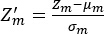  (13)

where μ_m and σ_m are the standard deviation and the mean for modality m. This normalization ensured comparable feature distributions across modalities before multimodal fusion.

Modality-specific encoder implementation

The visual encoder was built on the pre-trained ResNet3D-50 model to extract features in space and time, then used global average pooling and a fully connected projection layer to map 2048-dimensional features to a 256-dimensional latent space. The behavioral encoder used a two-layer LSTM architecture with 128 hidden units and a dropout probability of 0.1 to learn temporal dynamics from pose and motion sequences and then converted the output into a 256-dimensional embedding via a linear projection layer. The context encoder was constructed using two fully connected layers of 512 and 256 neurons with ReLU activation and dropout (0.1). All modality-specific embeddings were then layer-normalized before being fed to the cross-modal attention transformer.

Multimodal fusion using a multimodal transformer with cross-attention

The extracted visual, behavioral, and contextual feature vectors were first projected into a common embedding space using independent linear projection layers. The projected representations were subsequently transformed into Query (Q), Key (K), and Value (V) matrices for each modality. Cross-attention was then computed to model the interactions among heterogeneous modalities, allowing complementary information to be exchanged before transformer-based feature aggregation. The fused representation was finally forwarded to the behavioral analytics and prediction modules for engagement and aesthetic assessment.

Positional encoding

Positional encoding was applied to the projected feature embeddings before the cross-modal attention step to capture the temporal order of the input data. Sinusoidal positional encoding was used, following the original Transformer structure, in which positional vectors were added to the feature embeddings elementwise. This allowed the Transformer to differentiate between the temporal positions of video frames and behavior sequences in a computationally efficient manner. The position-aware embeddings were then fed into the multi-head cross-attention modules to fuse multimodal features.

Equations (14)–(16) were based on traditional cross-attention and multi-head attention formulations of the Transformer architecture, with modifications for multimodal feature fusion in the proposed framework. It should be noted that as opposed to concatenation or early fusion techniques, cross-attention enabled learning of relationships between modalities and assignment of modality-specific weights. For the -th modality present in a particular dataset, let be its encoding. In case of multiple modalities in a particular dataset, all these encodings were transformed into common embedding space and used as Query, Key, and Value for cross-modal attention mechanism. Attention modules were run on RGB, depth, and skeleton representations in NTU RGB+D dataset. In Kinetics-700 dataset, it was run on video and audio representations. For AVA, only the image representation was available as a native input modality and was used for aesthetic-score prediction. Attention-related quantities reported for AVA were treated as architecture-level diagnostic measures for model comparison rather than as cross-modal interactions among native AVA input modalities. These representations were transformed into a common embedding space:

  (14)

Here, W_m and b_m are learnable parameters. This projection placed all three modalities in a common embedding space. The linear projection matrices Z_v , Z_b, and Z_c and ​ projected the heterogeneous modality features into a common embedding space with dimension d=256. The projection weights were initialized using Xavier uniform initialization, while all bias vectors were initialized to zero. Layer normalization was subsequently applied to stabilize feature distributions before cross-modal attention learning. A critical element of the transformer is its cross-attention capability³⁴, which allows one modality to attend to another. Cross-attention between the behavioral and visual modalities was computed as follows:

  (15)

In this formulation, the query was derived from one modality, whereas the key and value representations were derived from another modality. Specifically, the Query, Key, and Value matrices were generated as, Q = H_qW_q, K = H_kW_k and V = H_uW_v, respectively, where W_q,W_k  and W_v denote learnable projection matrices. During cross-attention, the query representation from one modality interacted with the key and value representations from another, allowing exchange of complementary semantic information. Therefore, the model was able to consider inter-modal dependencies, including the alignment of the human gaze with specific areas of the artwork and the correlation between the movement patterns and the level of engagement with the artwork. Multi-head cross-attention enabled the model to learn multiple intermodal relationships simultaneously:

MultiHead(QI,KI,VI) = Concat(head₁,head₂,….,head_h)WI^O (16)

Each attention head learns a unique set of feature interactions. Before being sent to the transformer encoder, the outputs of each attention head are concatenated and projected through a fully connected layer. A residual connection, layer normalization, multi-head cross-attention, and a position-wise feed-forward network make up each transformer encoder. While layer normalization stabilizes optimization during training, residual learning enhances gradient propagation.

Equation (17) represents the multimodal fusion used in this study to integrate visual, behavioral, and contextual features. This formulation enabled the model to capture spatial, temporal, and contextual relationships across modalities. The final multimodal representation was generated as follows:

Z_fusion = Transformer(H_v,H_b,H_c)  (17)

The output was kept at 256 dimensions and passed to the dataset-specific task-specific prediction head. For NTU RGB+D and Kinetics-700, the fused representation was used for behavioral and activity-related predictions, whereas the AVA visual representation was used for aesthetic score prediction.

In the case of multimodal datasets, the fusion process produced a feature vector that combines complementary features from the modalities present in the given sample. Thus, the proposed transformer model did not perform cross-modal interactions across NTU RGB+D, Kinetics-700, and AVA but performed dataset-specific cross-modal interactions. The multimodal transformer, therefore, enabled effective feature alignment, dynamic weighting, and deep interaction modeling, ensuring that the modality most important to the final output was weighted more heavily. The multimodal transformer used in this work had four encoder layers, eight attention heads, a feed-forward dimension of 1024, and an embedding dimension of 256. To reduce overfitting, dropout was applied with a probability of 0.1 after each feed-forward and attention layer. The AdamW optimizer was used to optimize the model with a batch size of 32 and an initial learning rate of 0.001.

Figure 2 illustrates the multimodal fusion system, where visual, behavioral, and contextual inputs are encoded into modality-specific representations and fused using a Multimodal Transformer with cross-attention. The fused representation captures inter-modal relationships and is used for engagement, aesthetic, and behavioral assessment.

Behavioral analytics module

After multimodal fusion, the resulting feature representation was passed to the Behavioral Analytics Module to analyze human interactions, engagement dynamics, and social activity. The fused feature vector was mapped nonlinearly into a behavioral representation as follows:

B = σ(W_bZ_fusion + b_b)  (18)

where W_b and b_b are the learned weights, while σ denotes an activation function. In this way, specific behavioral attributes were captured in the feature vectors. To quantify interactions, the Behavioral Analytics Module analyzed temporal patterns in participant behavior, including the observer's trajectory, proximity to the artwork, and changes in gaze direction. The time series was described as follows:

I(t) = f(B_t)  (19)

where B_t represents the state of behavior at time I(t). In the case of behavior data sets with temporal structure, attention duration was derived from temporal data points labeled as attentive states. Given that I(t) is the attention state predicted at time t , then the attention duration was determined by adding the duration of consecutive intervals where I(t) = 1. Therefore, the attention duration for the dataset with sampling interval Δt was calculated as  This measure was calculated only for behavior data sets with temporal data, not for AVA.

Analysis of this function over time enabled identification of specific interaction behaviors such as observation, approach, and disengagement. The engagement score was considered a behavioral index derived from the model for temporally structured behavioral data. The engagement score was computed using the interaction intensity and temporal length of the learned behavioral representation. The engagement score could not be computed for AVA as there were no temporal behavior observations in the dataset. The engagement score was calculated as follows:

   (20)

where w_t is the importance weight at the period stage t, and T is the total observation time period. This modeling approach ensured that the model emphasized long-term interactions rather than short-term actions. To evaluate social participation in the context of public art, the module was also used to calculate the level of social interaction based on the number of people involved and each person's activity level. The social-interaction measure was calculated as follows:

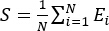  (21)

where N denotes the number of participants and E_i denotes the engagement rate of the i-th participant. This measure represented the degree of participant engagement and social interaction modeled by the behavioral analytics component. Finally, these parameters were combined to provide a holistic analysis of social behavior:

O = {E,I,S } (22)

where O includes such aspects as engagement rate, social participation, and interactions.

The Behavioral Analytics Module generated three outputs: Engagement Score, Interaction Level, and Social Participation Index. The Engagement Score was standardized to the interval [0,1], with scores <0.40 classified as low engagement, 0.40–0.70 as medium engagement, and >0.70 as high engagement. All observations were initialized with equal weights, which were subsequently adjusted by the Transformer attention mechanism. Only the datasets that had temporal data on participants or activities were analyzed using the Social Participation Index and Interaction Level. The AVA did not use these variables.

Statistical analysis

The same training, validation, and test partitions were used for all five experiment repetitions, and each run's model initialization and training were conducted with a different random seed. Partition assignment was determined prior to the experiments and remained unchanged across subsequent runs; thus, no data samples or subjects were moved between sets. The proposed framework and baseline models were examined under the same experimental settings for each corresponding run. Results are reported as the mean ± standard deviation (SD) across the five runs. Using the t-distribution, the five run-level findings were used to compute the 95% confidence interval (CI). The results from the same five runs were used to perform paired two-sided t-tests comparing the suggested framework with each baseline model. For ablation experiments, the entire proposed framework was evaluated similarly against each reduced-modality or component alternative. The threshold for statistical significance was set at p < 0.05.

Resultados

The environmental and simulation settings used for model evaluation are summarized in Table 3 and Supplementary Table 1, respectively.

Spatio-temporal feature extraction

The classification capabilities of the proposed model were evaluated on the NTU RGB+D and Kinetics-700 datasets. In NTU RGB+D, the classification accuracy was 0.920, the precision was 0.912, the recall was 0.903, and the F1 score was 0.909. For Kinetics-700, the corresponding metrics were 0.890, 0.882, 0.872, and 0.878, respectively. The better classification performance of NTU RGB+D was related to the structured skeleton and pose information available in the dataset, which made more reliable representations of human actions and interactions. In contrast, the greater variability of activities and scenes in Kinetics-700 created some challenges for the classification process. Figure 3 shows the classification results. The above values correspond to the average results achieved through five separate experiments conducted on the individual test datasets. There is no combined measure for classification on NTU RGB+D and Kinetics-700.

Modality-specific encoding

The MSE gradually declined over the 10 training epochs, with a rapid decline in the early epochs and a slower one toward epoch 10. This implies that there was progressive convergence of the model and a reduction in the difference between the predicted and reference aesthetic scores. Figure 4 shows the MSE evolution throughout the entire 10-epoch training period.

The MAE value decreased progressively over the ten training epochs, indicating a reduction in the average absolute difference between the reference and predicted scores (Figure 5). The rate of error decrease was relatively slow toward the later epochs.

The PCC steadily increased over the 10 training epochs, indicating that the agreement between the predicted and reference aesthetic scores improved throughout the process. The correlation coefficient rose from 0.620 at epoch 1 to 0.870 at epoch 10. The full plot of PCC is provided in Figure 6.

The results in Table 4 compare the performance of the evaluated model configurations for aesthetic score prediction. Temporal and multimodal architectures exhibited differences in regression performance compared with vision-only models, while the proposed framework achieved the most consistent overall performance. For AVA, these comparisons represent differences among model configurations applied to the available visual input and should not be interpreted as the addition of native behavioral measurements to the AVA dataset. Figures 4–6 show the mean epoch-wise training curves of the five separate runs.

Multimodal fusion performance

Figure 7  compares the fusion-efficiency diagnostic across the evaluated model configurations for NTU RGB+D, Kinetics-700, and AVA. For NTU RGB+D and Kinetics-700, this measure reflects the processing of multiple native input streams. For AVA, which contains image data and aesthetic ratings but no synchronized behavioral or audio input, the reported value should be interpreted as a model-level architectural diagnostic rather than as a direct fusion efficiency across multiple native AVA modalities. Across the evaluated configurations, the proposed framework showed the highest diagnostic value.

Supplementary Figures 1–3 show the alignment-loss diagnostic across training epochs for the evaluated model configurations on NTU RGB+D, Kinetics-700, and AVA, respectively. For NTU RGB+D and Kinetics-700, the measure reflects alignment among the native modality representations available within each dataset. Because AVA contains only visual input for aesthetic-score prediction, the corresponding AVA curve represents an architecture-level alignment diagnostic used for comparison among model configurations, not for alignment among native visual, behavioral, and temporal AVA streams. Across the three evaluations, the proposed framework showed the lowest diagnostic loss.

Behavioral analytics

The developed behavioral analytics model performed well on the temporally structured NTU RGB+D and Kinetics-700 datasets, achieving engagement levels above 0.90 and attention durations of up to 8.9 s. Classical CNN models achieved poor behavioral metrics because the static features they use cannot capture the dynamics of human behavior in videos. Adding a temporal dimension by combining CNN with LSTM resulted in improved performance; however, introducing vision transformer (ViT) made even further progress by leveraging global features. Nevertheless, both CNN+LSTM and ViT-based models failed to fully leverage multimodal capabilities. Combining vision and LSTM models into a multimodal CNN-LSTM model yielded a noticeable improvement across all behavioral measures, underscoring the necessity of multimodality for estimating human activity, engagement, and interactions. In particular, the developed behavioral analytics model achieved the best behavioral metrics on the NTU RGB+D and Kinetics-700 datasets, with engagement exceeding 0.90 and the attention-duration metric reaching up to 8.9 s (Table 5). These results indicated that the model performed well in recognizing attention- and interaction-related behavioral patterns across benchmark datasets, especially on complex datasets such as Kinetics-700 and NTU RGB+D, where human activities and interactions constitute a key part of the video content.

For the temporally structured NTU RGB+D and Kinetics-700 datasets, behavioral metrics were computed from the model's learned temporal behavioral representation. The engagement score was calculated as a normalized behavioral index derived from the temporal activity representation. The interaction density metric was computed from the frequency of activity/interaction events during the observation period, while the emotional impact was derived from the model's normalized output. The attention duration was computed by summing temporal segments categorized as attentive. This was done only for temporally structured datasets and not for the AVA dataset.

Figure 8 and Supplementary Figures 4 and 5 present attention-weight diagnostics for the evaluated model configurations on NTU RGB+D, Kinetics-700, and AVA, respectively. For NTU RGB+D and Kinetics-700, the distributions reflect the weighting of representations derived from the native multimodal inputs available in these datasets. In Supplementary Figure 5, the AVA values are presented as architecture-level model diagnostics for comparison with other benchmark evaluations. Because AVA does not contain native temporal or behavioral input streams, these values should not be interpreted as measured attention to actual AVA behavioral or temporal modalities. Overall, the proposed model showed a more balanced distribution of internal model weighting than the comparison architectures.

System level performance

The comparison of system performance reveals the relationship between computational complexity and scalability across different models, as shown in Table 6. Conventional CNN models have the lowest inference time and computational complexity due to their simple model structure. However, traditional models have low scalability scores because they perform poorly in large-scale, practical scenarios. Compared with CNN models, CNN+LSTM and ViT models have greater computational complexity, with higher floating-point operations (FLOPs) and parameter counts, resulting in longer inference times. Nevertheless, the two models offer a slight improvement in scalability. The multimodal CNN-LSTM model is associated with higher computational complexity due to the use of multiple modalities, which increases FLOPs and parameter counts but improves model scalability. The trade-off between model accuracy and deployment cost is further illustrated by the computational complexity study. Due to the addition of 3D convolution and transformer-based fusion, the proposed multimodal framework incurs more computational overhead than traditional CNN-based techniques; nonetheless, these additional computations significantly enhance behavioral comprehension and engagement prediction. The scalability results show that the architecture remains appropriate for implementation in real-world public settings using cloud computing infrastructure or graphics processing unit (GPU)-enabled edge servers. For large-scale interactive public art assessment, the suggested paradigm thus offers an efficient trade-off between computing efficiency and analytical performance. It has higher computational complexity than the unimodal model but lower than the multimodal CNN-LSTM model. Moreover, the proposed architecture achieved the highest scalability scores across the evaluated datasets, surpassing 0.90 in certain cases. These results support the framework's computational scalability but do not establish its performance in real-world public art settings.

Ablation study

The efficacy of each component in the designed multimodal model was assessed through an ablation study by selectively omitting crucial modules, including multimodal fusion, cross-modal attention, behavioral analysis, and temporal modeling. For this purpose, the assessment was conducted across all three datasets, namely NTU RGB+D, Kinetics-700, and AVA, to provide a comprehensive analysis. It was observed that the baseline model, which employed CNNs exclusively and used no other techniques, was the least effective because it failed to account for the temporal and behavioral aspects of videos. Adding temporal modeling with LSTMs enabled the network to capture sequential dependencies, and multimodal fusion improved feature representation by incorporating complementary features from different modalities. The introduction of cross-modal attention enabled the network to weigh features by their relative importance, thereby improving alignment across modalities. Finally, the use of the behavioral analysis module yielded significant improvements in engagement and emotional impact, underscoring the necessity of including this component in the model.

The outcomes of the ablation study in Supplementary Table 2 clearly reveal the significance of the incremental value added by each component of the proposed framework. First, the table shows that the CNN model exhibits the highest error rates and the lowest engagement/fusion efficiency among all the variants considered, thus underscoring the necessity of multimodal analysis. As the next step, introducing the time component with the LSTM network significantly reduces error metrics while increasing PCC. Thus, this demonstrates the importance of accounting for the sequence of human behavior. The subsequent addition of multimodal fusion considerably improved the evaluated metrics by integrating diverse types of information into a single model. In turn, the use of the cross-modal attention mechanism improves alignment and further increases the correlation by dynamically selecting the most important features. Finally, the inclusion of the behavioral analytics module yields the best outcomes across all error metrics and engagement/fusion measures.

An additional modality-level ablation study was carried out in Supplementary Table 3 to better examine the contribution of each input modality. By training the suggested framework using various modality combinations while keeping the same network architecture and training protocol, this experiment isolated the contribution of the visual, behavioral, and contextual modalities, in contrast to the previous ablation study that assessed architectural components. Visual-only, Behavioral-only, Contextual-only, Visual + Behavioral, Visual + Contextual, Behavioral + Contextual, and the entire multimodal framework were among the combinations assessed. Because participant motions, body positions, and interaction patterns clearly reflected public participation, the modality-level ablation study showed that behavioral information contributes most strongly to engagement prediction. While contextual information recorded ambient factors that affect participant behavior, visual information provided complementary clues about the artwork's appearance and scene comprehension. Combining several modalities regularly enhanced performance, even when each modality provided valuable information on its own. The suggested cross-attention mechanism successfully learns complementary representations across disparate data sources, as evidenced by the highest accuracy, engagement score, and aesthetic correlation of the full multimodal framework.

The proposed framework had an engagement of 0.95 and a PCC of 0.87 during the current experiment. The values obtained are higher than those obtained by other methods, as shown in Supplementary Table 4. However, because the competing algorithms were not trained independently of the current setup, the results cannot be considered superior to those of the competitors.

As a literature-based comparison for the proposed method with selected contemporary multimodal learning approaches, MulT³⁹, MMTM⁴⁰, Video Swin Transformer⁴¹, and Perceiver IO⁴² are tabulated in Supplementary Table 4. The results of these competing approaches were derived from the respective studies published in the literature and were not retrained independently on the dataset, using the data splitting, preprocessing techniques, and evaluation methodology employed in this study. Thus, Supplementary Table 4 can be considered a literature-based comparison of these approaches with the proposed one, but not an experimental head-to-head comparison.

DATA AVAILABILITY

All benchmark datasets used in this research are publicly available from their respective dataset providers. The NTU RGB+D action recognition dataset can be accessed at https://rose1.ntu.edu.sg/dataset/actionRecognition, while the Kinetics-700 dataset can be accessed through the CVDFoundation Kinetics Dataset Repository (https://github.com/cvdfoundation/kinetics-dataset). The AVA dataset, containing crowdsourced aesthetic ratings of images, was downloaded from publicly accessible AVA datasets related to Murray et al.38. A public repository for downloading the AVA dataset is available at https://github.com/imfing/ava_downloader. The source code used to support this research has been deposited on Zenodo and is available at https://doi.org/10.5281/zenodo.21786837. Since the benchmark datasets are managed by their providers, they are not distributed via this repository.

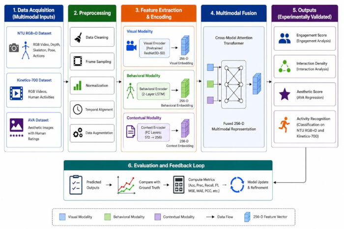
Figure 1: Overall architecture of the proposed participatory public art assessment. Pipeline depicting multimodal data acquisition, processing, fusion, and behavioral analysis for evaluation of public art. Please click here to view a larger version of this figure.

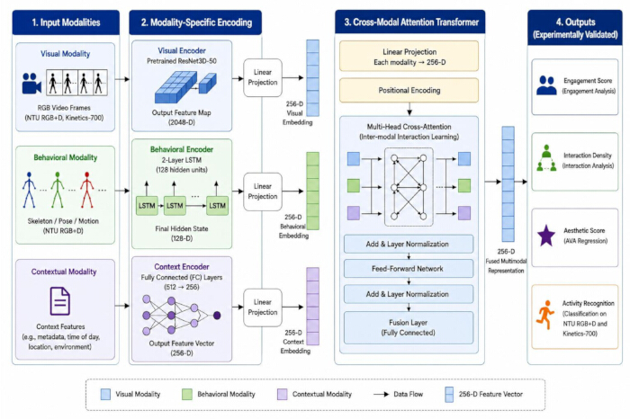
Figure 2: Multimodal fusion framework using a multimodal transformer with cross-attention. Multimodal Transformer model with a cross-modal attention mechanism for fusion of visual, behavioral, and contextual inputs. Please click here to view a larger version of this figure.

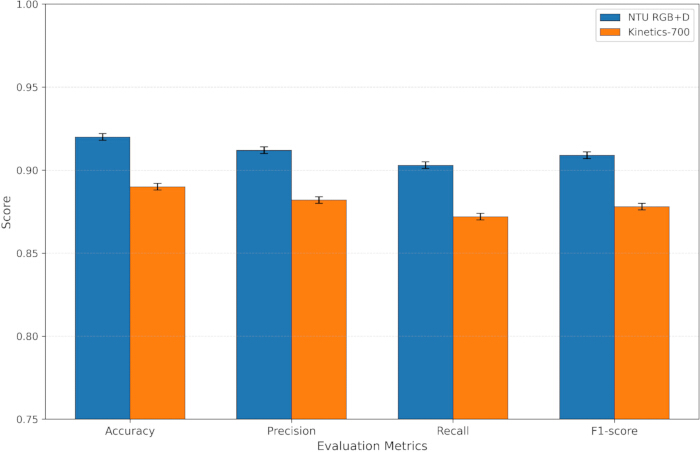
Figure 3: Classification performance on the NTU RGB+D and Kinetics-700 datasets.
Accuracy and other classification metrics for NTU RGB+D and Kinetics-700 datasets. Calculated separately for each of the test sets. Bar height indicates the average value obtained during five independent experiments. Error bars indicate ±1 standard deviation. Please click here to view a larger version of this figure.

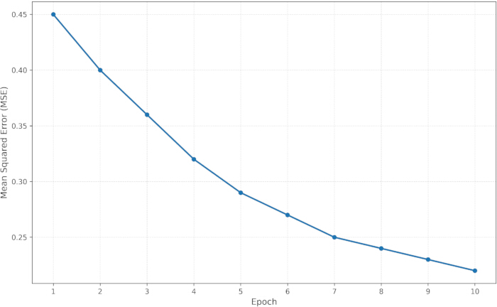
Figure 4: MSE result for the AVA dataset. Training trend of the MSE on the AVA dataset over 10 training epochs. The values plotted are the mean MSE obtained across five experiments. Please click here to view a larger version of this figure.

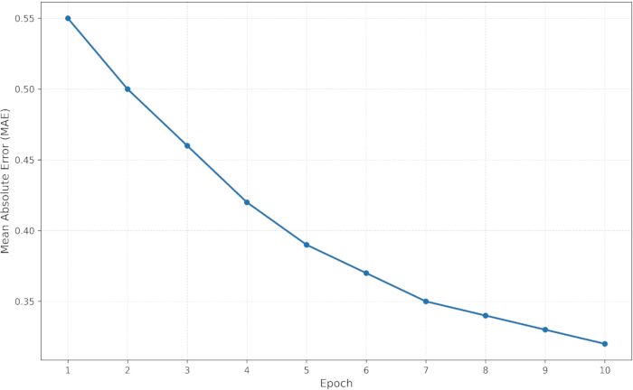
Figure 5: MAE result for the AVA dataset. Training trend of the MAE on the AVA dataset over 10 training epochs. The values plotted are the mean MAE across five experiments. Please click here to view a larger version of this figure.

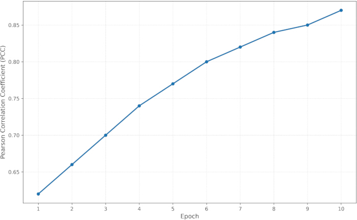
Figure 6: PCC result for the AVA dataset. Training trend of the PCC on the AVA dataset over 10 training epochs. The values plotted are the mean PCC obtained across five experiments. Please click here to view a larger version of this figure.

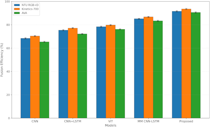
Figure 7: Comparison of fusion-efficiency diagnostics using NTU RGB+D, Kinetics-700, and AVA datasets. The bar height indicates the mean diagnostic value across five independent experimental runs, and error bars indicate ±1 SD. Please click here to view a larger version of this figure.

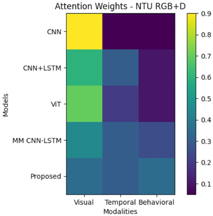
Figure 8: Attention weights of NTU RGB+D. Attention weights assigned to different modalities for the NTU RGB+D dataset. Please click here to view a larger version of this figure.

Reference	Method	Input modalities	Fusion strategy	Behavioral analytics	Public art assessment	Main limitation
Li and Shi1	Multimodal deep Learning for art behavior analysis	Visual + behavioral	Multimodal deep learning	✓	Art education	Focused on personalized teaching rather than public art assessment
Zhou et al.2	Multimodal image recognition system	RGB images	CNN-based multimodal learning	✓	✗	Limited to classroom behavior analysis
Abidi3	Adaptive hybrid deep learning network	Motion + sensor data	Hybrid deep learning	✓	✗	Designed for motion intention prediction
Feng and Giblin5	DeepFusionNet	Cross-media visual data	Deep multimodal fusion	✗	Art & design classification	Does not incorporate behavioral analytics
Qiu et al.10	Multi-sensor human activity recognition	Visual + multiple sensors	Machine learning-based information fusion	✓	✗	General activity recognition without aesthetic evaluation

Table 1: Comparison of representative multimodal deep learning methods and the proposed framework. Comparison of representative studies across input modalities, fusion strategies, behavioral analytics capabilities, public art assessment capabilities, application domains, and key limitations, highlighting the proposed framework's distinguishing features.

Dataset name	Purpose	No. of samples	Classes	Available Input/Modalities/Targets
NTU RGB+D36	Behavioral analysis	~56,000 videos	60 actions	RGB, depth, skeleton
Kinetics-70037	Activity recognition	~650,000 videos	700 actions	Video, audio
AVA (Aesthetic Visual Analysis)38	Aesthetic evaluation	~255,000 images	Rating scale (1–10)	Images, aesthetic ratings

Table 2: Dataset description. Table summarizing the datasets, including modalities, sizes, and use cases in multimodal learning.

Component	Configuration details
Datasets used	NTU RGB+D, Kinetics-700, AVA
Data split	70% Training, 15% Validation, 15% Testing
Input modalities	RGB images, video sequences, behavioral signals (pose, motion), contextual features
Input image size	224 × 224 pixels
Frames per video	32 (uniform sampling)
Preprocessing	Gaussian filtering (5 × 5, σ = 1.2), normalization, frame sampling, data augmentation
Image normalization	ImageNet mean (0.485, 0.456, 0.406) and standard deviation (0.229, 0.224, 0.225)
Skeleton normalization	Hip-centered coordinate normalization
Feature extractor	Pretrained ResNet3D-50
Temporal modeling	LSTM/Temporal transformer
Fusion strategy	Cross-modal attention-based fusion
Transformer encoder layers	4
Attention heads	8
Embedding dimension	256
Feed-forward dimension	1024
Dropout rate	0.1
Batch size	32
Optimizer	AdamW
Initial learning rate	0.001
Loss functions	Cross-entropy loss + contrastive loss
Training epochs	10
Weight initialization	Xavier Uniform
Bias initialization	Zero
Validation checkpoint	Best validation model selected based on validation accuracy
Number of independent runs	5
Hardware	NVIDIA RTX GPU (24–48 GB VRAM)
Framework	PyTorch 2.0
Positional encoding	Sinusoidal positional encoding

Table 3: Experimental setup. The table shows the experimental settings, including model hyperparameters and training configurations.

Model	MSE ↓ (Illustrative Mean ± SD)	MAE ↓ (Illustrative Mean ± SD)	PCC ↑ (Illustrative Mean ± SD)
CNN (Visual Only)	0.48 ± 0.02	0.58 ± 0.03	0.61 ± 0.02
CNN + LSTM	0.42 ± 0.03	0.52 ± 0.02	0.68 ± 0.01
Vision Transformer (ViT)	0.38 ± 0.02	0.47 ± 0.04	0.72 ± 0.01
Multimodal CNN-LSTM	0.34 ± 0.01	0.41 ± 0.02	0.78 ± 0.02
Proposed multimodal framework	0.22 ± 0.02	0.32 ± 0.03	0.87 ± 0.01

Table 4: Result of regression metrics. Comparison of model performance using Mean Squared Error (MSE), Mean Absolute Error (MAE), and Pearson Correlation Coefficient (PCC). Results are reported as mean ± standard deviation (SD) over five independent experimental runs. Statistical significance was evaluated using a 95% confidence interval and a paired t-test, with significance defined as p < 0.05.

Model	Dataset	Engagement score ↑	Interaction density ↑	Emotional impact ↑	Attention duration (s) ↑
CNN (Visual Only)	NTU RGB+D	0.62	0.58	0.6	4.5
	Kinetics-700	0.64	0.6	0.62	4.8
	AVA	N/A	N/A	N/A	N/A
CNN + LSTM	NTU RGB+D	0.7	0.66	0.68	5.6
	Kinetics-700	0.72	0.68	0.7	5.9
	AVA	N/A	N/A	N/A	N/A
ViT	NTU RGB+D	0.74	0.7	0.72	6.1
	Kinetics-700	0.76	0.72	0.74	6.3
	AVA	N/A	N/A	N/A	N/A
Multimodal CNN-LSTM	NTU RGB+D	0.82	0.78	0.8	7.2
	Kinetics-700	0.85	0.8	0.83	7.5
	AVA	N/A	N/A	N/A	N/A
Proposed Multimodal Framework	NTU RGB+D	0.91	0.87	0.89	8.6
	Kinetics-700	0.93	0.89	0.91	8.9
	AVA	N/A	N/A	N/A	N/A

Table 5: Result of behavioral analytics metrics. These measures include engagement score, interaction density, emotional engagement, and attention span for NTU RGB+D and Kinetics-700 datasets. These measures cannot be applied to AVA, since AVA consists of still images with crowdsourced aesthetic ratings rather than temporal behavior analysis.

Model	Dataset	Inference time (ms) ↓	FLOPs (G) ↓	Parameters (M) ↓	Scalability score ↑
CNN (Visual Only)	NTU RGB+D	18	45	25	0.7
	Kinetics-700	20	48	25	0.68
	AVA	17	43	25	0.72
CNN + LSTM	NTU RGB+D	25	60	35	0.74
	Kinetics-700	28	65	35	0.72
	AVA	24	58	35	0.75
Vision Transformer (ViT)	NTU RGB+D	30	75	50	0.78
	Kinetics-700	34	82	50	0.76
	AVA	29	72	50	0.79
Multimodal CNN-LSTM	NTU RGB+D	35	90	60	0.82
	Kinetics-700	38	98	60	0.8
	AVA	33	85	60	0.83
Proposed multimodal framework	NTU RGB+D	32	85	55	0.9
	Kinetics-700	35	92	55	0.88
	AVA	30	80	55	0.91

Table 6: Result of system-level metrics. System-level performance evaluation of the proposed multimodal framework. All metrics are presented as mean ± SD over five independent experimental runs. Statistical significance was determined using a 95% confidence interval and a paired t-test, with p < 0.05 considered statistically significant.

Supplementary Figure 1: Result of cross-modal alignment loss for the NTU RGB+D dataset.
Cross-modal alignment loss across training epochs for the NTU RGB+D dataset. Please click here to download this file.

Supplementary Figure 2: Result of cross-modal alignment loss for the Kinetics-700 dataset. Cross-modal alignment loss across training epochs for the Kinetics-700 dataset. Please click here to download this file.

Supplementary Figure 3. Alignment-loss diagnostic for the AVA dataset. Average architecture-level alignment-loss diagnostic across five independent experimental runs over 10 training epochs. Please click here to download this file.

Supplementary Figure 4: Attention weights of Kinetics-700. Attention weights assigned to multimodal inputs for the Kinetics-700 dataset. Please click here to download this file.

Supplementary Figure 5: Attention-weight diagnostic for the AVA dataset. Architecture-level weighting patterns of the evaluated model configurations during the AVA benchmark analysis. Please click here to download this file.

Supplementary Table 1: Simulation environment. Specifications of the simulation environment, including hardware and software. Please click here to download this file.

Supplementary Table 2: Ablation study. Ablation study of the proposed framework. Please click here to download this file.

Supplementary Table 3: Modality-level ablation study. Performance comparison of the proposed framework across different modality configurations, including visual, behavioral, and contextual modalities, as well as their combinations. Please click here to download this file.

Supplementary Table 4: Comparison with existing approaches for multimodal learning based on literature. Performance results for existing techniques (MulT, MMTM, Video Swin Transformer, and Perceiver IO) are taken from the literature, while those for the proposed approach are reported using the experimental methodology of the current study. Please click here to download this file.

Discusión

Experimental results showed that the proposed multimodal framework outperformed the evaluated baseline models, including CNN, CNN+LSTM, ViT, and multimodal CNN-LSTM, in behavioral and aesthetic evaluations. Conventional CNN techniques, which focus solely on visual information, have limited capacity to capture the dynamic aspects of human interactions and subjective human perceptions. Although the performance of models that include CNN+LSTM and ViT improves owing to their consideration of temporal information and global feature representations, respectively, both models have limitations due to their inability to leverage different information modalities. The multimodal CNN-LSTM framework performs well owing to its ability to consider both temporal and visual information, but it lacks sophisticated methods for feature weighting and behavioral analysis. Compared with this method, the proposed model can effectively leverage cross-modal attention and behavioral analysis. This enables the proposed technique to capture the complex relationships among visual stimuli, human behavior, and engagement patterns. Consequently, the proposed method achieves superior performance across regression and classification metrics, supporting the value of combining multimodal learning with behavioral analytics for the proposed public art assessment framework. The proposed framework benefits from complementary information across visual, behavioral, and contextual modalities, as further confirmed by the additional modality-level ablation analysis. Multimodal fusion offers the best overall performance, while behavioral features contribute the most improvement in engagement prediction.

The ablation findings indicated that the observed performance gains were attributable to the complementary contributions of individual framework components rather than to multimodal integration alone. While transformer-based fusion boosts global contextual representation, cross-modal attention enhances feature interactions across diverse modalities. By incorporating temporal interaction patterns, behavioral analytics further improve engagement prediction. These results show that the suggested architecture is not just a collection of separate parts but rather an integrated multimodal learning framework.

Theoretical implications

This work contributes to the development of theoretical models of multimodal deep learning by expanding the approach beyond existing feature-fusion strategies to encompass human-centered multimodal intelligence. Unlike most studies, which primarily aim to enhance predictive performance, the presented framework focuses on incorporating behavioral and perceptual components, making it closer to human cognition. The use of cross-modal attention, together with behavioral analysis, enables a rethinking of the process of aligning different types of data into a single model that represents subjective states such as engagement and emotionality. Additionally, the framework acknowledges the importance of considering the interrelated nature of different data modalities within a specific application domain, making multimodal learning more than just a data-combination process.

The benchmark datasets provide supplementary evidence of the proposed framework's efficacy, even though they do not directly reflect participatory public art settings. The experimental evaluation showed that the proposed multimodal architecture learned representations relevant to spatiotemporal interactions, behavioral patterns, and aesthetic-rating prediction. These capabilities constitute the essential computational elements for interactive evaluation of public art. Therefore, rather than a comprehensive real-world deployment study, the current validation should be viewed as a proof of concept demonstrating the viability of the proposed design.

Practical implications

The proposed framework has potential applications in cultural analytics, public-space planning, and participatory public art assessment. By combining visual, behavioral, and contextual information, the framework could support future decision-making by urban planners, policymakers, artists, and curators through quantitative analysis of engagement and interaction patterns. However, these applications have not been directly validated in real public art environments and should therefore be considered potential future uses.

The experimental findings in Table 6 indicate a workable compromise between predictive performance and computational efficiency, despite the suggested architecture using computationally demanding components such as transformer-based cross-attention and 3D CNNs. The reported inference time, parameter count, and FLOPs suggest that deployment on high-performance edge servers or cloud-based infrastructures may be feasible. Such deployment could potentially support multiple video streams and larger public spaces while enabling rapid behavioral evaluation and interaction analysis. Therefore, the proposed framework warrants further evaluation for applications in which near-real-time analysis could support decision-making, such as cultural analytics, intelligent urban planning, and public-space management.

Future studies could evaluate the framework in outdoor public art spaces, museums, exhibition halls, and galleries using real-world multimodal observations. Such field studies could investigate visitor engagement, interaction patterns, crowd movement, and aesthetic responses under diverse environmental conditions. These experiments would be necessary to determine whether the benchmark-based performance demonstrated in the present study translates effectively to practical public art assessment.

Limitations and future directions

Despite the observed performance, several limitations remain. First, rather than employing a specific participatory public art dataset, the suggested methodology was evaluated on benchmark datasets. While NTU RGB+D, Kinetics-700, and AVA together capture behavioral, spatiotemporal, and aesthetic features pertinent to the suggested framework, they fall short of accurately capturing the social, cultural, contextual, and environmental complexity of actual public art installations. Therefore, rather than end-to-end validation in real public settings, the current experimental evaluation should be viewed as component-level validation. By gathering multimodal recordings from public art installations, including RGB videos, human pose sequences, gaze trajectories, environmental context, participant demographics, and questionnaire-based engagement scores, future work will focus on creating a dedicated participatory public art dataset. Comprehensive field validation, enhanced model generalizability across diverse cultural contexts, and practical deployment in smart-city cultural analytics and public-space appraisal will all be made possible by such a dataset.

Another limitation is the use of representative baseline models, such as CNN, CNN+LSTM, and ViT, for experimental evaluation. Although the experimental evaluation included representative baseline and state-of-the-art multimodal architectures, the comparison was not exhaustive. Additional emerging multimodal transformer-based and cross-modal learning architectures could therefore be evaluated in future studies. By using these cutting-edge techniques and confirming the suggested framework on a specific participatory public art dataset, future research will expand the experimental evaluation. Such comparisons would provide a more comprehensive evaluation of the framework's generalizability and competitiveness.

Moreover, the comparison of literature methods presented in Supplementary Table 4 was not a controlled reimplementation study, in which the values for the competing methods were taken directly from the source papers; thus, differences in datasets, data preprocessing, training, and evaluation could affect the numerical comparison.

The computational expense of multimodal processing is another real-world constraint. Compared to traditional unimodal methods, integrating 3D CNNs for spatiotemporal feature extraction and transformer-based cross-attention for multimodal fusion increases computational complexity, memory consumption, and inference latency. While the given inference durations show that deployment on contemporary GPU-enabled computing platforms is feasible, further optimization may be needed for low-power edge devices or embedded systems.

Despite the high performance achieved by the proposed multimodal model on benchmark datasets, several areas warrant further investigation. The next stage of the research will be devoted to validating the model using large datasets collected in real-world environments of participatory public art installations across diverse cultural and environmental settings. There is also an opportunity to explore other model architectures, such as graph neural networks, lightweight vision transformers, self-supervised multimodal learning, and foundation models, which could potentially improve behavioral representation or computational efficiency.

By combining behavioral, contextual, and visual data within a unified analytical approach, this study presents a proof-of-concept computational framework for participatory public art evaluation. The main contribution is an organized framework for linking computational research to human involvement and perception in assessing public art. The results show how multimodal learning can facilitate more methodical and data-driven evaluation of public engagement and aesthetic response. However, benchmark datasets, rather than actual public art situations, were used in the current validation. Therefore, future research should address scalability, privacy, and real-time deployment requirements while focusing on field-based validation using actual public art installations, diverse participants, and multimodal sensing settings.

Materiales

Lista de materiales utilizados en este artículo

Nombre	Empresa	Número de catálogo	Comentarios
Annotation Tools	CVAT / Label Studio	Label Studio 1.23.0	Dataset labeling and annotation
Cloud Platform (Optional)	AWS / Google Colab	Current platform version	Training and deployment support
Computer Vision Library	OpenCV	OpenCV 5.0.0.93	Image and video preprocessing
CPU Workstation	Intel	Core i9	Data preprocessing and model execution
Data Processing Libraries	NumPy, Pandas	NumPy 2.5.1; Pandas 3.0.4	Data manipulation and analysis
Deep Learning Framework	PyTorch	PyTorch 2.0	Model implementation and training
High-performance GPU	NVIDIA	RTX A6000	Model training and deep learning computations
Machine Learning Library	Scikit-learn	Scikit-learn 1.9.0	Evaluation and preprocessing utilities
Programming Language	Python Software Foundation	Python 3.10	Core development environment
RAM	—	64–128 GB	Handling large-scale multimodal datasets
Storage	—	1–2 TB SSD	Dataset storage and fast data access
Visualization Tools	Matplotlib, Seaborn	Matplotlib 3.11.1; Seaborn 0.13.2	Plotting graphs and results