Este estudio presenta un flujo de trabajo reproducible para optimizar diseños de exposiciones inmersivas mediante la combinación de recocido simulado adaptativo, selección de propuestas dependiente de etapas y control de recalentamiento. El diseño seleccionado se implementó en un entorno de exposición de realidad virtual y se evaluó utilizando métricas de costo espacial, registros del comportamiento de los participantes y calificaciones posteriores a la experiencia.
Se requiere una suscripción a JoVE para ver este contenido. Inicie sesión o comience su prueba gratuita.
Artículo de investigación
Optimización del diseño de espacios de exhibición inmersivos mediante el recocido simulado adaptativo con recalentamiento y evaluación mediante realidad virtual
En este artículo
Resumen
Resumen
Los espacios expositivos inmersivos requieren distribuciones que favorezcan una circulación eficiente, una orientación clara, una interacción equilibrada y una experiencia ambiental cómoda. Sin embargo, las distribuciones expositivas suelen desarrollarse mediante decisiones de diseño manual, lo que dificulta evaluar simultáneamente la longitud de las rutas, la accesibilidad visual, el riesgo de aglomeración, la comodidad ambiental y la distribución de nodos de interacción. En este estudio se desarrolló y evaluó un flujo de trabajo de optimización del diseño espacial basado en recocido simulado adaptativo con selección de propuestas dependiente de etapas y control de recalentamiento. Se construyó una sala expositiva inmersiva de 36 m x 24 m con seis zonas temáticas, corredores de transición, un área de descanso y múltiples nodos de interacción. Se compararon tres condiciones de distribución: distribución manual, distribución mediante recocido simulado estándar y distribución mediante recocido simulado adaptativo con recalentamiento. El modelo de optimización minimizó una función de costo espacial ponderada que incorporaba distancia recorrida, accesibilidad visual, aglomeración, comodidad ambiental y equilibrio de interacción. Las distribuciones seleccionadas se implementaron en escenas expositivas de realidad virtual y se evaluaron mediante registros del comportamiento de los participantes y calificaciones posteriores a la experiencia. El algoritmo adaptativo produjo un costo espacial final menor, un porcentaje de mejora mayor y menos iteraciones hasta la mejor solución que el recocido simulado estándar, con un aumento moderado del tiempo de cálculo. Los participantes asignados a la distribución adaptativa reportaron mayor satisfacción, una sensación de presencia más intensa, una orientación más clara, menor percepción de aglomeración y menor carga cognitiva, y completaron la ruta con una distancia caminada más corta, menos vacilaciones, mayor tiempo de permanencia y una cobertura más amplia en el mapa de calor. Estos hallazgos respaldan el flujo de trabajo como un enfoque de apoyo a la toma de decisiones para el escenario expositivo evaluado; no establecen una distribución expositiva óptima universal ni una superioridad sobre todas las metaheurísticas alternativas.
Introducción
Los espacios expositivos inmersivos combinan cada vez más el diseño espacial, los medios digitales, las pantallas interactivas y las tecnologías de realidad virtual para crear entornos en los que los visitantes no simplemente observan el contenido, sino que se desplazan a través de él, reaccionan ante él e interpretan la exposición como una experiencia espacial. En tales entornos, la calidad de la experiencia depende no solo de la riqueza del contenido visual o interactivo, sino también de la continuidad de la ruta, la visibilidad, la aglomeración, la comodidad ambiental y la distribución de las oportunidades de interacción. Por lo tanto, el diseño del espacio expositivo implica un problema multifactorial: un diseño debe guiar a los visitantes de manera eficiente, al tiempo que preserva la secuencia narrativa, la apertura perceptiva y las oportunidades de participación. Durante mucho tiempo, los estudios sobre el comportamiento en museos y exposiciones han demostrado que la experiencia del visitante está determinada por la organización espacial, la estructura de circulación y la accesibilidad interpretativa, y no únicamente por el contenido de las exhibiciones1.
La teoría de la configuración espacial proporciona una base útil para tratar la distribución de las exhibiciones como un problema de diseño susceptible de análisis. Desde esta perspectiva, el espacio no es un contenedor pasivo de objetos; organiza el movimiento, el encuentro, la visibilidad y la elección. La configuración arquitectónica puede influir en la forma en que las personas se desplazan por un entorno y en la facilidad con que comprenden las relaciones entre los espacios2. El análisis espacial basado en la visibilidad refuerza aún más esta visión al mostrar que los campos visuales y las relaciones de línea de vista pueden modelarse como características medibles de la cognición espacial y la navegación3. Estas ideas son particularmente relevantes para las exhibiciones inmersivas, ya que los visitantes deben integrar continuamente información visual, decisiones de recorrido, señales de interacción y estímulos ambientales mientras se desplazan por la exhibición.
Al mismo tiempo, las tecnologías inmersivas han ampliado las formas en que se pueden diseñar y probar los entornos de exhibición antes de su implementación física. Las interfaces virtuales e inmersivas permiten a investigadores y diseñadores examinar cómo los usuarios perciben y se comportan bajo condiciones espaciales controladas, posibilitando comparaciones de diferentes distribuciones mientras se mantiene constante el contenido y las condiciones ambientales4. Revisiones de aplicaciones de realidad virtual inmersiva muestran que la estructura espacial, el diseño de la interacción y la claridad de la tarea son determinantes importantes del compromiso del usuario y de la calidad del aprendizaje5. Evidencia metaanalítica también sugiere que el nivel y tipo de inmersión pueden influir en la sensación de presencia, pero la inmersión por sí sola no garantiza mejores resultados si el entorno está mal organizado o es difícil de navegar6.
La experiencia del usuario en una exposición inmersiva está estrechamente relacionada con la presencia, la carga cognitiva y la comodidad física. La presencia refleja en qué medida los usuarios experimentan que se encuentran dentro de un entorno mediado, lo que la convierte en un resultado clave en entornos virtuales e inmersivos7. Sin embargo, los entornos inmersivos también pueden generar una carga cognitiva cuando la navegación, la interacción o la información sensorial no están bien coordinadas8. Por este motivo, la optimización del espacio expositivo no debería limitarse a aumentar la densidad de interacción o la estimulación visual. Debe favorecer una experiencia espacial coherente, reducir decisiones innecesarias sobre rutas y minimizar la fatiga evitable. También debe vigilarse la cinetosis simulada, ya que el malestar puede afectar tanto a la seguridad de la exposición a la realidad virtual como a la interpretación de los resultados de la experiencia del usuario9.
A pesar de estos requisitos, muchos diseños de exposiciones aún se desarrollan a partir de la experiencia de los diseñadores, ajustes manuales iterativos u observaciones posteriores a la visita de los espectadores. Estos enfoques siguen siendo valiosos, pero dificultan la evaluación simultánea de múltiples restricciones de diseño. El diseño espacial para exposiciones inmersivas puede plantearse como un problema de optimización con restricciones que considere conjuntamente la longitud de la ruta, la visibilidad, la aglomeración, la comodidad y la distribución de interacciones. El recocido simulado es adecuado para este tipo de problema porque puede explorar espacios de solución grandes e irregulares, permitiendo al mismo tiempo la aceptación controlada de soluciones intermedias no mejoradas, ayudando así a escapar de óptimos locales10. Su lógica de aceptación sigue la regla de Metrópolis11, mientras que el marco más general de Metrópolis-Hastings introduce una razón entre las densidades de propuesta hacia adelante y hacia atrás cuando el núcleo de propuesta es asimétrico12. En la implementación actual, los cuatro núcleos de propuesta condicionales son simétricos; por lo tanto, la derivación formal muestra que la razón de Hastings es igual a uno para movimientos factibles reversibles. En consecuencia, el método se describe como recocido simulado adaptativo con aceptación de Metrópolis y recalentamiento, y no como un muestreador de Metrópolis-Hastings independiente.
Durante mucho tiempo, las variantes del recocido simulado adaptativo han empleado selección no uniforme de vecindarios, modificación de los programas de enfriamiento, recalentamiento, estrategias de reinicio y componentes de búsqueda híbridos13,14. Por lo tanto, la presente implementación debe interpretarse como una configuración específica de la aplicación y no como una nueva primitiva metaheurística. Su contribución radica en el acoplamiento explícito de un programa de propuestas de cuatro movimientos dependiente de la etapa y el recalentamiento con restricciones de factibilidad específicas de la exhibición, una función de costo espacial transparente de múltiples componentes y una validación en realidad virtual a nivel de participante15. Esta posición más restringida distingue directamente el presente flujo de trabajo de las afirmaciones sobre un principio de optimización fundamentalmente nuevo. Se esperaba que la selección de propuestas dependiente de la etapa desplazara la búsqueda desde una exploración más amplia de secuencias/rutas hacia un refinamiento espacial local, mientras que el recalentamiento restauraba la movilidad de la búsqueda tras una estancación. Se esperaba que este equilibrio entre exploración y explotación redujera el atrapamiento prematuro en mínimos locales y aumentara la probabilidad de alcanzar una distribución factible de menor costo dentro del mismo presupuesto nominal de iteraciones.
Este estudio propone un flujo de trabajo reproducible que integra recocido simulado adaptativo, selección de propuestas dependiente de la etapa, control de recalentamiento, un modelo espacial de costos multifactorial y evaluación en realidad virtual a nivel de participante. La contribución metodológica está orientada a aplicaciones y centrada en la reproducibilidad, más que en afirmar un principio de optimización fundamentalmente nuevo16. El método compara un diseño manual, un diseño mediante recocido simulado estándar y un diseño mediante recocido simulado adaptativo con recalentamiento, en un entorno de exposición controlado en realidad virtual. El estudio examina tanto los resultados algorítmicos como los resultados a nivel de participante, incluyendo el costo espacial final, el porcentaje de mejora, la sensación de presencia, la claridad de orientación, la satisfacción, la carga cognitiva, la distancia recorrida, la cantidad de vacilaciones, el tiempo de permanencia, y la cobertura del mapa de calor. La hipótesis principal fue que el método adaptativo alcanzaría un costo espacial final menor que el recocido simulado estándar; a nivel de participante, se esperaba que el diseño correspondiente mejorara la satisfacción general y la eficiencia de la ruta en comparación con los diseños manual y mediante recocido simulado estándar. Esta perspectiva sigue la lógica general de los métodos de diseño metaheurísticos, en los que la búsqueda computacional apoya, más que sustituye, el juicio humano en el diseño17.
Acceso restringido. Inicie sesión o comience una prueba gratuita para ver este contenido.
Protocolo
The study protocol was reviewed by Henan Agricultural University and was determined to be exempt from formal ethics review on December 20, 2025. No separate ethics approval or exemption reference number was issued by the reviewing body. Written informed consent was obtained from all participants before enrollment.
Participant preparation
Adult participants aged 18–60 years with normal or corrected-to-normal vision were recruited. Participants who reported severe vestibular disorders, uncontrolled epilepsy, severe visual impairment, recent major surgery, or previous serious discomfort during virtual-reality exposure were excluded. Each participant completed a screening form before the experiment. Age group, gender, education level, prior virtual-reality experience, and prior museum or exhibition-visiting frequency were recorded as control variables.
Participants were assigned to one of three layout conditions using a computer-generated randomization list: manual layout, standard simulated annealing layout, or adaptive simulated annealing with reheating layout. A between-subject design was used to avoid learning effects across layouts. The allocation ratio was set to 1:1:1, with 60 participants assigned to each condition and 180 participants in total. Age group, gender, education level, previous virtual-reality experience, and museum/exhibition-visiting frequency were recorded before allocation for descriptive assessment of participant characteristics; these variables were not used as post-randomization exclusion criteria.
Exhibition-space model preparation
A rectangular immersive exhibition hall measuring 36 m x 24 m with a ceiling height of 4.5 m was constructed. The total usable floor area was set to 864 m2. One entrance and one exit were placed on opposite short sides of the hall. Both the entrance and exit widths were set to 3.0 m and were kept fixed across all layout conditions.
The exhibition hall was divided into six thematic exhibition zones, two transition corridors, one rest area, and one main visitor route. The allowable area for each thematic zone was set to 80–130 m2, and the rest-area allocation was set to 40 m2. The allowable main-pathway width was set to 1.8–3.5 m. Eight to twelve interaction nodes were placed in each layout. Each interaction node was defined as a point where participants could stop, activate digital content, view an exhibit, or change direction.
The floor plan was discretized into 0.5 m x 0.5 m grid cells. The grid was used for visibility analysis, route-continuity checking, heatmap coverage calculation, and local density estimation. Each thematic zone was represented by its center coordinate, boundary polygon, area, and route-sequence position. Each interaction node was represented by its coordinate, associated zone, trigger radius, and clearance area.
Spatial configuration was treated as the core design variable because exhibition layout, visibility, and route structure affect visitor movement, wayfinding, and spatial cognition18. The complete workflow, from spatial model construction to layout optimization, virtual-scene implementation, participant testing, and statistical analysis, is shown in Figure 1.
Layout parameters and feasibility constraints
The same feasibility constraints were applied to all layout conditions. First, all thematic zones were required to remain inside the 36 m x 24 m boundary. Second, thematic zones were not allowed to overlap. Third, the main visitor route was required to connect the entrance, six thematic zones, a rest area, and the exit without interruption. Fourth, interaction nodes were not allowed to block the main path. Fifth, each interaction node was required to retain a clearance radius of at least 1.2 m. Sixth, the predicted local density on the main route was required to be no more than 1.50 persons/m2. Seventh, the final route was required to contain no dead ends or disconnected subpaths.
The same scene scale, route rules, environmental targets, and interaction settings were used across the three layout conditions. Before the optimization algorithms were run, the hall dimensions, functional-zone parameters, pathway-width range, interaction-node settings, feasibility thresholds, virtual-reality settings, objective-function weights, algorithm parameters, and outcome definitions were recorded. These parameters defined the reproducible boundary of the protocol and are summarized in Table 1.
Spatial-cost function
Each candidate layout was evaluated using the weighted spatial-cost function:

where F(x) is the total spatial cost of layout x. Cdistance(x) is the walking-distance cost, Cvisibility(x) is the visual-accessibility cost, Ccrowding(x) is the crowding cost, Ccomfort(x) is the environmental-comfort penalty, and Cinteraction(x) is the interaction-balance penalty. A lower F(x) indicates a more favorable layout.
The walking-distance cost was calculated as:

where Lx is the total route length of layout x in meters. A reference maximum route length of 120 m was used.
The visual-accessibility cost was calculated as:
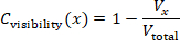
where Vx is the thematic-zone frontage visible from the main route, and Vtotal is the total frontage length of all thematic zones. Line-of-sight rays were emitted every 0.5 m along the visitor route. Exhibition partitions, walls, and zone boundaries were treated as occluding objects.
The crowding cost was calculated as:
Ccrowding(x) = min(Dmax / 1.50, 1)
where Dmax is the maximum predicted local density in persons/m2. An upper density threshold of 1.50 persons/m2 was used for the main route.
The environmental-comfort penalty was calculated as:

The illuminance penalty was set as:
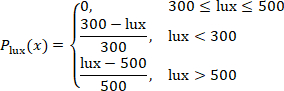
The sound-pressure penalty was set as:
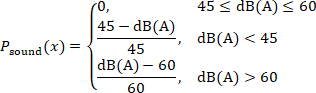
The carbon dioxide penalty was set as:

The temperature penalty was set as:
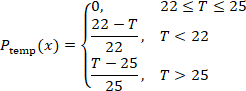
The interaction-balance penalty was calculated as:

where sk is the route distance between two adjacent interaction nodes. A lower value indicates a more even distribution of interaction opportunities along the visitor route.
Environmental comfort is included because lighting, sound, air quality, and temperature influence fatigue, comfort, and willingness to remain in exhibition environments19. The environmental ranges are protocol control targets rather than universal regulatory limits. The 300–500 lx illuminance band is consistent with current Chinese building and museum-lighting guidance; the carbon-dioxide target of <900 ppm is deliberately more conservative than the 1,000 ppm daily-average limit in GB/T 18883-202220,21; the 22–25 °C temperature band is within commonly accepted thermal-comfort conditions for lightly active occupants22; and 45–60 dB(A) is used as a controlled ambient-sound band rather than as a statutory indoor-noise limit23,24.
The objective-function weights were selected as explicit, scenario-specific design priorities rather than as universal coefficients or preference estimates fitted from participant outcomes. Walking distance and crowding each received a weight of 0.25 because route efficiency and congestion control were treated as the two primary operational constraints; visual accessibility received 0.20 because visibility affects orientation and exhibits exposure; environmental comfort and interaction each received 0.15 so that these factors influence the search without dominating circulation-related terms. Because exhibition priorities can differ by context, the protocol tests local weight robustness by perturbing each weight by ±10% individually and proportionally renormalizing the remaining weights so that the total remains 1.00. The resulting coefficients should therefore be interpreted as protocol-specific design settings that can be recalibrated for artistic, historical, scientific, or commercial exhibitions.
Manual layout generation
The manual layout was created as the baseline condition. The six thematic zones were arranged in a conventional narrative sequence from entrance to exit. The rest area was placed near the middle section of the route. The initial main-pathway width was set to 2.2 m. Interaction nodes were placed near the entrance of each thematic zone and at major route-turning points. The manual layout was checked against all feasibility constraints. Zone boundaries were adjusted only when a constraint was violated. After the layout became feasible, total route length, visible frontage ratio, maximum local density, environmental-comfort penalty, interaction-spacing coefficient, and total spatial cost were recorded.
Standard simulated annealing
The feasible manual layout was used as the initial state. The initial temperature was set to 100, the cooling coefficient to 0.95, the maximum number of iterations to 1,500, and the stagnation threshold to 200 iterations. The algorithm was run with 30 independent random seeds. These values were operational protocol settings used to define a matched computational budget; they were not presented as literature-derived universal constants or outcome-tuned optima. T₀ = 100 permitted broad early exploration, α = 0.95 provided gradual cooling, 1,500 iterations provided each run with the same upper search budget, and the 200-iteration stagnation threshold prevented prolonged continuation after no improvement. The same temperature and maximum-iteration settings were used for the adaptive method so that differences were attributable to proposal scheduling and reheating rather than to a larger nominal search budget.
At each iteration, one neighboring layout was generated by applying one move: moving one thematic zone by 0.5–2.0 m, swapping the sequence positions of two thematic zones, adjusting one pathway segment by 0.1–0.3 m, or moving one interaction node by 0.5–1.5 m. A proposed layout was rejected immediately if it violated any feasibility constraint.
If the proposed layout was feasible and had a lower spatial cost, it was accepted. If it had a higher spatial cost, it was accepted according to the probability equation:
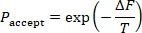
where ΔF is the increase in spatial cost, and T is the current temperature. The temperature after each iteration was updated using:
Tnew = 0.95Told
Each run was stopped when the maximum iteration count was reached or when the best spatial cost did not improve for 200 consecutive iterations. Simulated annealing was considered suitable for this task because exhibition layout optimization is a combinatorial spatial problem that cannot be solved efficiently by exhaustive search.
Standard simulated annealing was used as the primary numerical algorithmic benchmark because it shared the same layout encoding, feasibility rules, objective function, initialization, temperature schedule, and computational budget as the adaptive condition. Standard simulated annealing was the sole numerical metaheuristic comparator in this study and therefore functioned as a matched ablation-like baseline for the added proposal scheduling and reheating at the workflow level. Genetic algorithms, particle swarm optimization, ant colony optimization, and learning-based optimizers were not part of the experiment; accordingly, performance claims were restricted to the matched standard-SA baseline. For each run, the random seed, initial spatial cost, final spatial cost, improvement percentage, number of iterations to the best solution, runtime, acceptance rate, and feasibility status were stored. Improvement percentage was calculated using the equation:

Adaptive simulated annealing with reheating
The same initial layout, feasibility constraints, initial temperature, cooling coefficient, maximum iteration count, and 30 random seeds as the standard simulated annealing condition were used. The adaptive algorithm differed only in its stage-dependent move-class probabilities and reheating rule, while retaining the standard Metropolis acceptance rule for feasible candidate layouts. Four proposal move classes were defined: local displacement (L), zone-sequence swap (S), pathway-width adjustment (W), and interaction-node relocation (N). During the first 40% of iterations, the move-class probabilities were set to pL = 0.20, pS = 0.35, pW = 0.30, and pN = 0.15. During the final 60%, they were set to pL = 0.35, pS = 0.15, pW = 0.20, and pN = 0.30. This change in move-class frequency shifted the search from broader sequence/pathway exploration toward local spatial refinement and adjustment of interaction nodes.
At iteration t, the full proposal density was expressed as q(x′|x,t) = pm(t)qm(x′|x), where m ∈ {L,S,W,N} represented the selected move class and pm(t) represented its phase-specific probability. For local displacement, one of six thematic zones was selected uniformly, a displacement direction was drawn uniformly on [0,2π), and a displacement magnitude was drawn uniformly on [0.5,2.0] m; therefore, qL was proportional to (1/6)(1/2π)(1/1.5). For a zone-sequence swap, one of the 15 unordered zone pairs was selected uniformly, giving qS = 1/15. For pathway-width adjustment, one of J adjustable pathway segments was selected uniformly, and a signed change was drawn uniformly from [−0.3,−0.1] ∪ [0.1,0.3] m, giving qW = (1/J)(1/0.4). For interaction-node relocation, one of K current interaction nodes was selected uniformly, a direction was drawn uniformly on [0,2π), and a displacement magnitude was drawn uniformly on [0.5,1.5] m, giving qN proportional to (1/K)(1/2π)(1/1.0). Constraint-violating proposals were rejected and contributed a self-transition.

For every reversible feasible move in this implementation, the conditional proposal kernel was symmetric: qm(x′|x) = qm(x|x′). Because the same phase-specific move-class probability pm(t) was applied to the forward and reverse transition at a given iteration, q(x|x′,t)/q(x′|x,t) = 1. The acceptance probability, therefore, is reduced to the standard simulated-annealing Metropolis rule, A(x→x′) = min{1, exp[−(C(x′)−C(x))/T]}. No non-trivial Hastings correction was applied; the method is therefore termed adaptive simulated annealing with reheating rather than a Metropolis-Hastings sampler25.
Reheating was applied when the best spatial cost did not improve for 150 consecutive iterations, thereby intentionally intervening before the 200-iteration stagnation stop used in standard simulated annealing. The current temperature was increased by 10%, and up to 3 reheating events were allowed per run. The same algorithm-performance variables as in the standard simulated annealing condition were stored. The experiment evaluated the combined stage-dependent proposal schedule plus reheating configuration and therefore did not estimate the independent causal contribution of each component. Stepwise pseudocode for the exact proposal, feasibility, Metropolis acceptance, temperature update, reheating, and output storage sequence was provided in Supplementary File 3.
Treheated = 1.10Tcurrent
Final layouts
One final layout was selected for each condition. The feasible manual layout was used for the manual condition. Under the standard simulated annealing conditions, the run with the lowest final spatial cost among the 30 runs was selected. For the adaptive simulated annealing with reheating condition, the feasible run with the lowest final spatial cost among the 30 runs was selected. Before the selected layouts were exported, a final feasibility check confirmed that all zones were inside the boundary, no zones overlapped, the route was continuous, the entrance and exit were unchanged, interaction-node clearance was at least 1.2 m, maximum density remained below 1.50 persons/m2, and all thematic zones were reachable from the main route.
Virtual exhibition scenes
Three virtual exhibition scenes were built in Unity 2022.3.22f1 LTS (Unity Technologies) using XR Interaction Toolkit 2.5.4. The scenes were presented through a Meta Quest 2 head-mounted display (Meta Platforms) using six-degree-of-freedom head and controller tracking. Exhibition content, visual style, object models, signage style, lighting assets, ambient sound, interaction mechanism, and navigation instructions were kept identical across the three scenes. Only spatial arrangement, route sequence, pathway width, and interaction-node placement varied.
The virtual camera height was set to 1.65 m, and the walking speed was set to 1.2 m/s. Teleportation was disabled. The same starting trigger at the entrance and the same completion trigger at the exit were used. The interaction-node trigger radius was set to 1.0 m. Whether each interaction node was visited was recorded.
The same six thematic contents were used in all scenes. Each theme was assigned to its corresponding zone, regardless of layout conditions. Wall height, partition style, media display size, text density, and exhibit object scale were kept constant. Virtual-reality environments were considered appropriate for this protocol because they enabled the examination of spatial presence, route clarity, and visitor experience under controlled layout conditions26.
The hardware, software, environmental-monitoring tools, questionnaire/codebook files, and analysis resources required to reproduce the protocol were listed in the Table of Materials and organized as Supplementary Files 1–3. Research resources with registered Research Resource Identifiers (RRIDs) were listed by RRID in the Table of Materials.
Participant session
One participant was tested at a time. The participant sat for 2 min before the session. The head-mounted display was fitted, and the interpupillary distance was adjusted according to the participant's comfort. A 2 min practice scene that was not part of the exhibition was provided. The practice scene was used only to familiarize the participant with movement and interaction.
Because one participant was tested at a time, crowding in the protocol was represented by model-based density estimates rather than emergent simultaneous group movement. Multi-user co-presence, interpersonal avoidance, and dynamic crowd interactions were therefore not directly simulated and were considered when interpreting crowd-related outcomes.
After practice, the assigned exhibition scene was started. The participant was instructed to enter the exhibition, follow the route naturally, interact with marked nodes, and exit after completing all six thematic zones. Additional route guidance was provided only if the participant could not proceed for more than 30 s. Completion time, dwell time, walking distance, hesitation count, interaction-node visits, and trajectory coordinates were recorded automatically.
The session ended when the participant reached the exit trigger. The head-mounted display was removed, and the participant was allowed to rest for 3 min. The participant completed the post-experience questionnaire immediately after the rest period.
Behavioral, environmental, and questionnaire outcomes
Completion time was defined as the time from entrance-trigger activation to exit-trigger activation. Dwell time was defined as the total time spent inside thematic zones and interaction-node areas. Walking distance was defined as cumulative path length from trajectory coordinates. Hesitation count was defined as the number of pauses longer than 3 s outside interaction-node areas. Heatmap coverage was calculated using:

Average illuminance was recorded using a Testo 540 illuminance meter (Testo SE & Co. KGaA), sound pressure level using a Testo 816-1 Class 2 sound level meter (Testo SE & Co. KGaA), carbon-dioxide concentration using a Testo 535 CO₂ measuring instrument (Testo SE & Co. KGaA), and ambient temperature using a Testo 605i thermohygrometer (Testo SE & Co. KGaA). The same monitoring positions were used across the three scene conditions. Illuminance was recorded in lx, sound pressure level in dB(A), carbon dioxide in ppm, and temperature in °C.
Presence and spatial-presence domains were measured using the 7-point scoring structure specified in the study protocol. These constructs were interpreted with reference to the validated Presence Questionnaire (PQ) framework of Witmer and Singer and the Igroup Presence Questionnaire (IPQ) framework of Schubert et al.27. The study variables were reported as domain-level 7-point scores rather than as standard PQ or IPQ total scores. For simulator sickness, the Simulator Sickness Questionnaire symptom framework was used together with the prespecified 0–30 study summary variable; higher values indicated greater discomfort. This 0–30 study summary was reported separately from the standard weighted SSQ Total Severity score, consistent with the distinction between simulator-sickness measurement conventions and cybersickness reporting28. Interaction quality, wayfinding clarity, visual comfort, acoustic comfort, thermal comfort, perceived crowding, cognitive load, and overall satisfaction were measured using the study-specific, multi-item, 7-point rating scales. Supplementary File 2 documented the construct source, score range, and reporting convention for each domain.
Study outcomes
The primary algorithmic outcome was defined as the final spatial cost. The primary visitor-experience outcome was defined as overall satisfaction. Secondary algorithmic outcomes were defined as the improvement percentage, the number of iterations to the best solution, the runtime, and the acceptance rate. Secondary visitor-experience outcomes were defined as presence, spatial presence, interaction quality, wayfinding clarity, visual comfort, acoustic comfort, thermal comfort, perceived crowding, cognitive load, simulator sickness, completion time, dwell time, walking distance, hesitation count, and heatmap coverage. Completion time and walking distance were used to evaluate route efficiency. Hesitation count and wayfinding clarity were used to evaluate navigation quality. Presence, spatial presence, interaction quality, and dwell time were used to evaluate immersive engagement. Perceived crowding, cognitive load, comfort ratings, and simulator sickness were used to evaluate experiential burden.
Data cleaning and quality control
All participant records were checked before analysis. It was confirmed that each record had a single participant identifier, a single condition label, complete behavioral logs and questionnaire scores, and no duplicate identifiers. Presence, spatial-presence, and study-specific experience ratings were restricted to their defined 1–7 ranges. The simulator-sickness study summary variable was restricted to its prespecified 0–30 range. The questionnaire/codebook file was checked to confirm that it documented the construct source, response range, domain construction, and derived-score definitions used in the analysis.
A participant record was excluded if the session was not completed, completion time was less than 3 min or greater than 25 min, heatmap coverage was less than 10%, the trajectory log was incomplete or technically invalid, walking distance was less than 20 m in conjunction with an incomplete/invalid trajectory record, or the participant requested early termination. No upper walking-distance cutoff was applied; walking distance was retained as a continuous study outcome across its valid observed range. An algorithm run was excluded from layout selection if it violated any feasibility constraint. Random seeds, layout files, algorithm outputs, questionnaire/codebook files, and analysis scripts were preserved for reproducibility. Random-seed preservation was necessary because stochastic optimization outputs could vary with initialization and proposal behavior29.
Algorithm performance
The 30 standard simulated annealing runs and 30 adaptive simulated annealing with reheating runs were analyzed. Initial spatial cost, final spatial cost, improvement percentage, iterations to best solution, runtime, and acceptance rate were summarized as mean ± standard deviation (SD), and 95% confidence intervals were reported for the group means and between-algorithm differences.
Normality was assessed using quantile-quantile (Q-Q) plots and the Shapiro-Wilk test. Homogeneity of variance was assessed using Levene's test. The two algorithmic conditions were compared using independent-samples t tests when assumptions were met. Mann-Whitney U tests were used when assumptions were not met. Two-sided p values, 95% confidence intervals, and effect sizes were reported. Cohen's d was calculated using the equation

where:

Rank-biserial correlation was used for nonparametric comparisons. Sensitivity analysis was conducted by changing each objective-function weight by ±10% individually and proportionally renormalizing the remaining four weights so that the total remained 1.00. The final spatial cost and improvement percentage were recalculated for each alternative weight vector. The algorithmic comparison was considered stable when the adaptive simulated annealing with reheating condition retained a lower final spatial cost across the alternative weight settings.
Participant outcome analysis
Participant outcomes across the three layout conditions were analyzed using IBM SPSS Statistics 27.0 (IBM Corp.). Continuous variables were reported as mean ± SD, and categorical variables were reported as counts and percentages. Normality was assessed using Q-Q plots and the Shapiro-Wilk test. Homogeneity of variance was assessed using Levene's test. One-way analysis of variance (ANOVA) was used for normally distributed outcomes with acceptable homogeneity of variance. Welch's ANOVA was used when the assumption of homogeneity of variance was violated. Kruskal-Wallis tests were used for non-normal outcomes.
Pairwise comparisons were conducted among the manual layout, standard simulated annealing layout, and adaptive simulated annealing with reheating layout. The three pairwise comparisons within each outcome were adjusted using the Holm method. The 95% confidence intervals were reported together with adjusted p-values. Eta-squared was reported for standard ANOVA, omega-squared for Welch's ANOVA, epsilon-squared for Kruskal-Wallis tests, and standardized mean differences for pairwise comparisons. As a supplementary robustness analysis, pairwise Welch contrasts were calculated from the group mean, SD, and n = 60 per group. Welch degrees of freedom, two-sided p values, Holm-adjusted p values, 95% CIs for mean differences, and Hedges g were calculated. This supplementary analysis used the group-level statistics and was presented in Supplementary Table 1.
The randomized 1:1:1 three-group comparison was treated as the primary analysis. Age group, gender, education level, previous virtual-reality experience, and museum/exhibition-visiting frequency were recorded before allocation to characterize the sample and identify obvious imbalance. The trial was not designed or powered for subgroup interaction tests, and no prespecified moderator model was included; these characteristics were therefore treated as contextual variables rather than demonstrated moderators. Random allocation provided design-based control over baseline characteristics, while the residual influence of prior VR familiarity was explicitly retained as a limitation. Eta-squared was calculated using
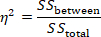
Epsilon-squared for Kruskal-Wallis tests was calculated as:
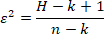
where H is the Kruskal-Wallis test statistic, k is the number of groups, and n is the total sample size.
Overall satisfaction, presence, wayfinding clarity, perceived crowding, cognitive load, completion time, walking distance, hesitation count, and heatmap coverage were prioritized in the interpretation because these variables directly reflected spatial efficiency and immersive visitor experience.
Acceso restringido. Inicie sesión o comience una prueba gratuita para ver este contenido.
Resultados
Flujo de participantes y completitud de los datos
Un total de 180 participantes completaron el experimento de exposición inmersiva y fueron incluidos en el análisis final. Las tres condiciones de distribución se equilibraron, asignando 60 participantes al diseño manual, 60 al diseño de recocido simulado estándar y 60 al diseño de recocido simulado adaptativo con recalentamiento. Ningún registro de participante fue excluido tras el control de calidad de los datos. Todos los registros conductuales y ...
Acceso restringido. Inicie sesión o comience una prueba gratuita para ver este contenido.
Discusión
El presente estudio evaluó un flujo de trabajo reproducible para el diseño de exposiciones que combina un modelo de costo espacial ponderado, recocido simulado adaptativo con recalentamiento y pruebas con participantes en realidad virtual. Dentro del escenario predeterminado de 36 m x 24 m, la distribución adaptativa logró un costo espacial menor que el recocido simulado estándar y se asoció con una mayor satisfacción, una presencia más intensa, una orientación más clara, rutas más cortas, menos vacilaciones y una cobert...
Acceso restringido. Inicie sesión o comience una prueba gratuita para ver este contenido.
Divulgaciones
Los autores declaran que no existen intereses financieros en conflicto.
Agradecimientos
Los autores agradecen a los participantes que tomaron parte en la evaluación de la exposición de realidad virtual. Los autores también agradecen a la Escuela de Arte y Diseño y a la Facultad de Ciencias de la Información y Gestión de la Universidad Agrícola de Henan por su apoyo en el desarrollo y evaluación del flujo de trabajo de diseño del espacio expositivo inmersivo. El estudio no recibió financiamiento externo. El trabajo fue apoyado por los recursos propios de los autores y por las instalaciones institucionales rutinarias de la Universidad Agrícola de Henan.
Acceso restringido. Inicie sesión o comience una prueba gratuita para ver este contenido.
Materiales
| Nombre | Empresa | Número de catálogo | Comentarios |
|---|---|---|---|
| Software de modelado 3D | Blender Foundation | N/A | Blender 4.0.2; utilizado para construir la geometría del espacio expositivo, zonas temáticas, particiones y activos espaciales. RRID:SCR_008606 |
| Scripts de análisis | Scripts de investigación personalizados | N/A | Versión 1.0; utilizados para análisis estadístico, análisis de sensibilidad, cálculos de intervalos de confianza y preparación de datos para figuras. |
| Monitor de dióxido de carbono | Testo SE & Co. KGaA | testo 535; 0563 0535 | Medidor digital de CO2; rango de medición 0–10,000 ppm; utilizado como verificación de control del protocolo de la concentración de dióxido de carbono bajo el objetivo ambiental predefinido. |
| Estación de trabajo de escritorio | Dell Technologies | Precision 3660 Tower | 32 GB de RAM; utilizada para renderizado de escenas virtuales, simulación de distribución, ejecución de algoritmos y registro de sesiones de participantes. |
| Scripts para generación de figuras | Scripts de investigación personalizados | N/A | Versión 1.0; utilizados para generar gráficos de rendimiento del algoritmo, gráficos de resultados de visitantes y mapas térmicos de trayectorias. |
| Motor de videojuegos/plataforma de realidad virtual | Unity Technologies | N/A | Unity 2022.3.22f1 LTS; utilizado para construir y ejecutar las escenas virtuales de la exposición. |
| Dispositivo de visualización montado en la cabeza | Meta Platforms, Inc. | Meta Quest 2 (128 GB) | HMD autónomo de 6 grados de libertad; 1832 × 1920 píxeles por ojo; frecuencia de actualización de sesión de 90 Hz; utilizado para presentar la escena inmersiva de realidad virtual y rastrear el movimiento del participante. |
| Medidor de iluminancia | Testo SE & Co. KGaA | testo 540; 0560 0540 | Medidor digital de lux; rango de medición 0–99,999 lx; utilizado como verificación de control del protocolo de iluminancia bajo el objetivo ambiental predefinido. |
| NumPy | Desarrolladores de NumPy | N/A | Versión 1.26.4; utilizado para operaciones numéricas con matrices y preparación de datos. RRID:SCR_008633 |
| Script de optimización | Script de investigación personalizado | N/A | Python 3.11, versión 1.0; implementa el recocido simulado estándar y el recocido simulado adaptativo con recalentamiento (Adaptive SA-R), incluyendo selección de propuestas dependiente de la etapa, aceptación de Metropolis y recalentamiento. |
| pandas | Equipo de desarrollo de pandas | N/A | Versión 2.1.4; utilizado para limpieza de conjuntos de datos, tabulación y preparación de datos listos para figuras. RRID:SCR_018214 |
| Formulario de cribado de participantes | Formulario de investigación personalizado | N/A | Versión 1.0; utilizado para registrar elegibilidad, variables demográficas, experiencia previa con realidad virtual y frecuencia de visitas a museos o exposiciones. |
| Cuestionario de valoración tras la experiencia | Formulario de investigación personalizado | N/A | Versión 1.0; escalas de respuesta de 7 puntos; utilizado para evaluar la calidad de la interacción, claridad de la orientación, comodidad visual/acústica/térmica, percepción de aglomeración, carga cognitiva y satisfacción general. |
| Formulario de valoración de presencia y presencia espacial | Formulario de investigación personalizado | N/A | Versión 1.0; puntuaciones específicas del estudio en dominios de 7 puntos interpretadas con referencia a los marcos PQ/IPQ; no se informaron puntuaciones totales estándar de PQ o IPQ. |
| Lenguaje de programación Python | Python Software Foundation | N/A | Versión 3.11; utilizado para ejecución de algoritmos, cálculo de funciones de costo, procesamiento de datos y análisis de sensibilidad. RRID:SCR_008394 |
| SciPy | Comunidad SciPy | N/A | Versión 1.11.4; utilizado para pruebas estadísticas y análisis numéricos complementarios. RRID:SCR_008058 |
| Formulario de valoración de cinetosis por simulador | Formulario de investigación personalizado | N/A | Versión 1.0; resumen del estudio preespecificado de 0–30 basado en el marco de síntomas de SSQ; distinto de la puntuación estándar ponderada de severidad total de SSQ. |
| Medidor de nivel de sonido | Testo SE & Co. KGaA | testo 816-1; 0563 8170 | IEC 61672-1 Clase 2; 30–130 dB; ponderación de frecuencia A/C; utilizado como verificación de control del protocolo del nivel de presión sonora bajo el objetivo ambiental predefinido. |
| Software de hojas de cálculo | Microsoft | N/A | Microsoft Excel 2021; utilizado para organización de conjuntos de datos, preparación de libros de códigos y archivos complementarios de hojas de cálculo. RRID:SCR_016137 |
| Software estadístico | IBM | N/A | IBM SPSS Statistics 27.0; utilizado para ANOVA, pruebas de Welch, verificación de supuestos y verificación estadística complementaria. RRID:SCR_002865 |
| Monitor de temperatura | Testo SE & Co. KGaA | testo 605i; 0560 2605 03 | Termohigrómetro; rango de temperatura −20 a +60 °C; resolución de 0,1 °C; utilizado como verificación de control del protocolo de la temperatura ambiente bajo el objetivo ambiental predefinido. |
| Paquete de integración de RV | Unity Technologies | N/A | XR Interaction Toolkit 2.5.4; utilizado para interacción en RV, control de movimiento, eventos de activación y registro de trayectorias. |
| NOTA: No se utilizaron recursos biológicos en este estudio. Se proporcionan RRID para los recursos de investigación aplicables. |
Referencias
- Falk JH, Dierking LD. The museum experience revisited. Left Coast Press; Walnut Creek, CA; 2013.
- Hillier B, Hanson J. The social logic of space. Cambridge University Press; Cambridge; 1984.
- Turner A, Doxa M, O'Sullivan D, Penn A. From isovists to visibility graphs: a methodology for the analysis of architectural space. Environ Plan B Plan Des. 2001;28:103-21.
- Kuliga SF, Thrash T, Dalton RC, Hölscher C. Virtual reality as an empirical research tool: exploring user experience in a real building and a corresponding virtual model. Comput Environ Urban Syst. 2015;54:363-75.
- Radianti J, et al. A systematic review of immersive virtual reality applications for higher education: design elements, lessons learned, and research agenda. Comput Educ. 2020;147:103778.
- Cummings JJ, Bailenson JN. How immersive is enough? A meta-analysis of the effect of immersive technology on user presence. Media Psychol. 2016;19:272-309.
- Witmer BG, Singer MJ. Measuring presence in virtual environments: a presence questionnaire. Presence-Teleop Virt. 1998;7:225-40.
- Makransky G, Petersen GB. The Cognitive Affective Model of Immersive Learning: a theoretical research-based model of learning in immersive virtual reality. Educ Psychol Rev. 2021;33:937-58.
- Kennedy RS, Lane NE, Berbaum KS, Lilienthal MG. Simulator Sickness Questionnaire: an enhanced method for quantifying simulator sickness. Int J Aviat Psychol. 1993;3:203-20.
- Kirkpatrick S, Gelatt CD Jr, Vecchi MP. Optimization by simulated annealing. Science. 1983;220:671-80.
- Metropolis N, et al. Equation of state calculations by fast computing machines. J Chem Phys. 1953;21:1087-92.
- Hastings WK. Monte Carlo sampling methods using Markov chains and their applications. Biometrika. 1970;57:97-109.
- Aarts EHL, Korst JHM. Simulated annealing and Boltzmann machines: a stochastic approach to combinatorial optimization and neural computing. John Wiley & Sons; Chichester; 1989.
- Van Laarhoven PJM, Aarts EHL. Simulated annealing: theory and applications. D. Reidel Publishing Company; Dordrecht; 1987.
- Bertsimas D, Tsitsiklis J. Simulated annealing. Stat Sci. 1993;8:10-5.
- Talbi EG. Metaheuristics: from design to implementation. John Wiley & Sons; Hoboken, NJ; 2009.
- Sörensen K. Metaheuristics: the metaphor exposed. Int Trans Oper Res. 2015;22:3-18.
- Hillier B. Space is the machine: a configurational theory of architecture. Cambridge University Press; Cambridge; 1996.
- Lolli F, et al. Post-Occupancy Evaluation's (POE) applications for improving indoor environment quality (IEQ). Toxics. 2022;10:626.
- Ministry of Housing and Urban-Rural Development of the People's Republic of China, State Administration for Market Regulation. GB/T 50034-2024 Standard for lighting design of buildings. Beijing; 2024.
- State Administration for Market Regulation, Standardization Administration of China. GB/T 23863-2024 Specification for lighting design of museum. Beijing; 2024.
- State Administration for Market Regulation, Standardization Administration of China. GB/T 18883-2022 Standards for indoor air quality. Beijing; 2022.
- Ministry of Housing and Urban-Rural Development of the People's Republic of China, General Administration of Quality Supervision, Inspection and Quarantine. GB/T 50785-2012 Evaluation standard for indoor thermal environment in civil buildings. Beijing; 2012.
- Ministry of Environmental Protection of the People's Republic of China, General Administration of Quality Supervision, Inspection and Quarantine. GB 3096-2008 Environmental quality standard for noise. Beijing; 2008.
- Chib S, Greenberg E. Understanding the Metropolis-Hastings algorithm. Am Stat. 1995;49:327-35.
- Slater M, Sanchez-Vives MV. Enhancing our lives with immersive virtual reality. Front Robot AI. 2016;3:74.
- Schubert T, Friedmann F, Regenbrecht H. The experience of presence: factor analytic insights. Presence-Teleop Virt. 2001;10:266-81.
- Stanney KM, Kennedy RS, Drexler JM. Cybersickness is not simulator sickness. Proc Hum Factors Ergon Soc Annu Meet. 1997;41:1138-42.
- Blum C, Roli A. Metaheuristics in combinatorial optimization: overview and conceptual comparison. ACM Comput Surv. 2003;35:268-308.
- Benedikt ML. To take hold of space: isovists and isovist fields. Environ Plan B Plan Des. 1979;6:47-65.
- Penn A. Space syntax and spatial cognition: or why the axial line? Environ Behav. 2003;35:30-65.
- Sherman WR, Craig AB. Understanding virtual reality: interface, application, and design. Morgan Kaufmann; San Francisco, CA; 2003.
- Slater M. Place illusion and plausibility can lead to realistic behaviour in immersive virtual environments. Philos Trans R Soc Lond B Biol Sci. 2009;364:3549-57.
- Sweller J. Cognitive load during problem solving: effects on learning. Cogn Sci. 1988;12:257-85.
- Heydarian A, Carneiro JP, Gerber D, Becerik-Gerber B. Immersive virtual environments versus physical built environments: a benchmarking study for building design and user-built environment explorations. Autom Constr. 2015;54:116-26.
- Rebenitsch L, Owen C. Review on cybersickness in applications and visual displays. Virtual Real. 2016;20:101-25.
- Clay V, König P, König SU. Eye tracking in virtual reality. J Eye Mov Res. 2019;12:3.
- Deb K, Pratap A, Agarwal S, Meyarivan T. A fast and elitist multiobjective genetic algorithm: NSGA-II. IEEE Trans Evol Comput. 2002;6:182-97.
- Kennedy J, Eberhart RC. Particle Swarm Optimization. Proc IEEE Int Conf Neural Netw. 4, 1942-1948.
- Dorigo M, Maniezzo V, Colorni A. Ant system: optimization by a colony of cooperating agents. IEEE Trans Syst Man Cybern B Cybern. 1996;26:29-41.
Acceso restringido. Inicie sesión o comience una prueba gratuita para ver este contenido.