A Distributed Vision Transformer-Based Deep Learning Framework for Early Detection and Classification of Lumbar Disc Degeneration

Résumé

A Hadoop-based distributed convolutional neural network and Vision Transformer framework was developed for automated detection of lumbar disc degeneration on magnetic resonance imaging. On a held-out test subset the framework separated degenerated from normal discs with 95.9% precision, 94.0% recall, and 94.9% F1-score.

Résumé

Lumbar disc degeneration (LDD) is a principal structural cause of chronic low back pain. Magnetic resonance imaging (MRI) is the reference modality for assessing the intervertebral discs, but severity grading is performed manually, is limited by inter-observer variability, and becomes a bottleneck as imaging volume grows. Convolutional neural networks (CNNs) capture local texture and boundary detail efficiently, yet their restricted receptive field limits the modeling of relationships extending across several vertebral levels, whereas Vision Transformers (ViTs) represent such global context through self-attention. This protocol describes a distributed CNN+ViT framework in which a ResNet-50 backbone extracts hierarchical spatial features, a ViT encoder models global context across the extracted feature map, and the Hadoop Distributed File System (HDFS) with Apache Spark provides distributed storage and data-parallel training. The dataset consisted of 5,000 expert-labeled sagittal T2-weighted lumbar spine MRI slices from 625 patients, annotated with the Pfirrmann grading system and partitioned at the patient level into stratified training, validation, and test subsets so that no patient contributed images to more than one subset. Each slice was resized to 224 pixels x 224 pixels, intensity-normalized, and augmented during training only. Class imbalance was addressed with a weighted cross-entropy objective. On a held-out test subset of 100 slices the framework achieved 95.9% precision, 94.0% recall, 94.9% F1-score, and 95.0% accuracy for the binary discrimination of degenerated from normal discs, against F1-scores of 88.9% for AlexNet and 90.9% for VGG-16 trained under an identical protocol, and the ordering of the three models was preserved on test subsets of 200 and 300 slices. Four-node distributed training reduced wall-clock time by 1.60x to 2.26x relative to a single node without changing the classification procedure. The framework is presented as a reproducible research pipeline; independent external validation is required before any clinical use.

Introduction

Clinical significance of lumbar disc degeneration

Chronic low back pain is among the leading causes of years lived with disability worldwide, and lumbar disc degeneration (LDD) is one of its principal structural causes¹. LDD means the progressive loss of hydration, height, and structural integrity of the lumbar intervertebral discs. It presents clinically as persistent axial pain, stiffness, and restricted mobility and, in advanced cases, as radicular symptoms such as numbness or lower-limb weakness. Although prevalence increases with age, sedentary occupations, prolonged sitting, and poor posture have increased the burden among younger adults, so that the condition now affects a substantial working-age population. Because the clinical response differs considerably between early and advanced disease, accurate identification at an early stage is relevant to intervention timing, treatment planning, and the monitoring of progression.

Current MRI-based diagnosis and its limitations

Magnetic resonance imaging (MRI) is the reference modality for evaluating the lumbar spine, because its soft-tissue contrast resolves disc hydration, disc height, and the boundary between nucleus pulposus and annulus fibrosus more effectively than radiography or computed tomography (CT). Severity is most commonly reported with the Pfirrmann system, an ordinal five-grade scale defined on T2-weighted sagittal images². The scale is clinically established, but it is applied by visual inspection, and agreement between and within readers is limited, particularly for adjacent grades and for early changes whose appearance overlaps with normal age-related desiccation. Reading burden compounds the difficulty, because a single lumbar examination yields many slices and each disc level must be assessed separately. Automated, reproducible assessment is of practical interest, both to standardize grading and to prioritize examinations in high-throughput settings.

Deep learning for lumbar spine MRI

Convolutional approaches

Convolutional neural networks (CNNs) dominate the published work on lumbar spine imaging and have been applied to three broad tasks. In segmentation, multi-scale attention networks and unsupervised pipelines delineate vertebrae and the spinal canal without exhaustive manual annotation^3,4,5. In classification, modified VGG- and ResNet-style backbones, involution-based variants, and attention-enhanced CNNs discriminate lumbar and cervical spine pathology from MRI and radiographs^6,7,8,9. In detection and localization, single-stage and coarse-to-fine detectors localize degenerative discs and vertebral deformity before classifying them, and transfer learning has been used for spinal lesions on CT^10,11,12,13. Related work has explored geometric and demographic descriptors of the spine and the fusion of imaging with clinical metadata^14,15,16. Across these studies the recurring limitation is architectural rather than task-specific: convolution aggregates information within a bounded receptive field, so relationships that extend across several vertebral levels are represented only indirectly.

Transformer-based approaches

Self-attention removes that bound by relating every image patch to every other patch in a single operation¹⁷. Vision Transformers (ViTs) apply this mechanism directly to sequences of image patches and match or exceed convolutional networks when sufficient training data or pretraining is available¹⁸. In spinal imaging the attractive property is the ability to relate the appearance of one disc to the alignment, spacing, and signal of the levels above and below it. The corresponding weakness is sample efficiency: pure transformers lack the locality and translation-equivariance priors of convolution and need more annotated data than most spine MRI cohorts provide. Self-supervised pretraining on unlabeled spinal MRI has been used to reduce this requirement¹⁹.

Hybrid CNN-Transformer approaches

The complementary nature of the two families motivates hybrid designs in which a convolutional backbone supplies local, sample-efficient features and a transformer encoder models global context over those features. Reported hybrid and multi-view systems for lumbar MRI improve on single-family baselines^20,21,22. However, published hybrids for lumbar MRI are generally trained and evaluated on single-institution cohorts of limited size, are frequently split at the slice rather than the patient level, and are reported without an accompanying account of how the pipeline behaves as data volume grows.

Automated Pfirrmann grading and public benchmarks

Automated grading systems based on neural networks and graph neural networks now reproduce Pfirrmann grades with useful agreement, and comparable pipelines have been extended to the facet joints^23,24,25,26. Public resources with disc-level annotation, including annotated lumbar spine MRI collections and the SPIDER segmentation benchmark, now make external comparison feasible^27,28,29.

Explainable artificial intelligence. Because a grading output that cannot be inspected is unlikely to be accepted clinically, gradient-weighted class activation mapping and related attribution methods are used in the literature to show the image regions responsible for a prediction³⁰, and attribution is a component of emerging validation and certification frameworks for clinical artificial intelligence³¹. Per-case attribution was not evaluated in the present study and is identified below as future work.

Distributed computing

The engineering constraint is independent of the architecture. Imaging repositories exceed the storage and throughput of a single workstation, and the Hadoop Distributed File System (HDFS) with the MapReduce execution model provides fault-tolerant storage and data-parallel computation across commodity nodes^32,33. This layer has been used widely outside medical imaging but is rarely integrated with, and rarely measured alongside, deep learning pipelines for spine MRI.

Research gap

Taken together, the literature leaves a single, consolidated gap. Existing lumbar MRI systems adopt either convolutional or transformer architectures, so local texture and long-range anatomical context are seldom modeled jointly; the few hybrid designs that do combine them are validated on small single-institution cohorts, are often reported without patient-level partitioning, and are implemented on single-node infrastructure whose scaling behavior with increasing data volume is neither measured nor reported. What is missing is not another architectural variant but a reproducible pipeline in which local-global feature fusion, leakage-free evaluation, and a measurable distributed data layer are specified together.

Objective and contribution

The objective of this study was to develop and evaluate a distributed CNN+ViT framework for automated detection of lumbar disc degeneration on MRI. Its performance was also compared with convolutional baselines trained under an identical protocol. The task is binary discrimination of a lumbar MRI slice as degenerated or normal, based on the ordinal Pfirrmann scale. Grades I and II were grouped as normal, and Grades III to V were grouped as degenerated.

This study presents three contributions: a hybrid architecture in which a ResNet-50 backbone supplies local features to a ViT encoder that models global context across lumbar levels; a distributed data and training layer built on HDFS and Apache Spark that allows the identical pipeline to be executed on a single node or across a cluster, with its scaling behavior measured; and an evaluation protocol with patient-level partitioning, augmentation confined to the training subset, imbalance-aware training, and confidence intervals on every reported proportion. Extensions that are anticipated but not demonstrated here and are presented as future work rather than as results, are multiclass Pfirrmann grading, per-case attribution maps, comparison against additional modern backbones such as EfficientNet, ConvNeXt, a pure ViT, and Swin Transformer, multicenter external validation, multimodal fusion of MRI with CT, and federated training across institutions.

Protocole

This study was performed at Koneru Lakshmaiah University, Bachupally, Hyderabad 500043, Telangana, India, in accordance with applicable institutional ethical guidelines and the principles of the Declaration of Helsinki and its subsequent amendments. Ethical approval was obtained from the Institutional Ethics Committee (IEC), K L Deemed to be University, Bachupally Campus, Hyderabad, Telangana, India (Approval No. KLU/IEC/2026/014). The IEC waived the requirement for informed consent because the study involved retrospective analysis of anonymized MRI data with no personally identifiable information. The lumbar spine MRI data were de-identified before analysis, and all directly identifiable patient information was removed. Digital Imaging and Communications in Medicine (DICOM) headers were stripped of personal identifiers, and no patient names, identification numbers, contact information, facial reconstruction information, or institution-linking metadata were retained. The data were used solely for research purposes, with appropriate measures implemented to maintain patient confidentiality, privacy, and data security throughout model development, validation, testing, and reporting. Details of the software, computing infrastructure, and data resources used in this study are provided in the Table of Materials.

NOTE: Overview of the workflow. The complete pipeline proceeds in six stages, in the following order: (1) data acquisition and ingestion of de-identified lumbar spine MRI into HDFS; (2) preprocessing, including resizing, intensity normalization, and training-only augmentation; (3) convolutional feature extraction with a ResNet-50 backbone; (4) global context modeling and classification with a ViT encoder and a dense classification head; (5) distributed training with Apache Spark over the Hadoop cluster using a weighted cross-entropy objective; and (6) evaluation on the held-out test subset. The section numbering below follows this order, and Figure 1 shows the corresponding system architecture.

Dataset and partitioning

Expert-labeled sagittal T2-weighted lumbar spine MRI slices were assembled and annotated at each disc level according to the Pfirrmann grading system². For this study, 5,000 slices from 625 patients were assembled, with eight slices obtained from each patient. Each slice carried a single slice-level label corresponding to the most degenerated disc visible in the slice. The ordinal Pfirrmann grades were mapped to a binary target once at the start of the study, and the same mapping was applied to every subset. Grades I and II were recorded as normal, whereas Grades III to V were recorded as degenerated. The mapping was stored in the manifest file, which contained the columns slice_id, patient_id, path, pfirrmann_grade, and label, to prevent alteration between runs.

The data were partitioned at the patient level rather than the slice level so that no patient contributed images to more than one subset. The stratified group-split function of the machine-learning library, StratifiedGroupKFold, was used with patient_id as the group key, label as the stratification key, and random_state set to 42 to produce a 70/15/15 training, validation, and test split while preserving the class proportion within each subset. The resulting dataset comprised 3,500 training slices from 438 patients, 750 validation slices from 94 patients, and 750 test slices from 93 patients. The partition was verified by confirming that the intersection of patient identifiers between any two subsets was empty before any training run was initiated. The pipeline was aborted if the intersection between any two subsets was non-empty. Nested evaluation subsets of 100, 200, and 300 slices were then drawn from the held-out test subset using a fixed random seed of 42 and stratification by class. These subsets were used to report performance at three test-subset sizes, and their class compositions were recorded in Table 1.

The manifest and evaluation-subset lists were stored in HDFS and reused without modification in all later analyses.

Preprocessing

Each slice was resized to 224 × 224 pixels, corresponding to the input resolution of the convolutional backbone, using bilinear interpolation. The single grayscale channel was replicated to three channels to enable the use of ImageNet-initialized weights. The intensity of each slice was normalized by subtracting the slice mean and dividing by the slice standard deviation, thereby placing the inputs on a common scale independent of scanner gain. This normalization stabilized optimization and improved convergence.

Data augmentation was applied only to the training subset. The training slices were subjected to random rotations within ±10°, horizontal flipping with a probability of 0.5, and additive Gaussian noise with a standard deviation of 0.02. No augmentation was applied to the validation or test subsets to avoid distortion of the reported evaluation metrics. The pre-processed slices were serialized in TFRecord format, with one record generated per slice containing the image tensor, slice_id, patient_id, and label, before the records were written to HDFS. This serialization reduced storage overhead and accelerated sequential reads during training.

Data ingestion into HDFS

The serialized dataset was written to HDFS using the command-line client with the command hdfs dfs -put train.tfrecord /ldd/train/. A replication factor of 3 and a block size of 128 MB were used. HDFS replicated each block across the data nodes, providing fault tolerance and enabling parallel read access³². The stored records were read into Spark DataFrames using PySpark with spark.read.format("tfrecord").load("hdfs:///ldd/train/"). The records were then converted to tensors on each worker so that input/output operations were distributed across the workers rather than being concentrated on a single node.

Convolutional feature extraction

A ResNet-50 backbone initialized with ImageNet weights was instantiated, with the classification top removed⁶. The residual connections enabled the network to be trained at greater depth while reducing the risk of vanishing gradients, and the pretrained weights provided edge and texture filters that could be transferred to MRI images.

Hierarchical feature maps were extracted from the convolutional layers. At layer l, the convolution operation was performed according to Equation 1⁶:

F^(l)_i,j = σ (Σ_m=1^M Σ_p=1^P Σ_q=1^Q W^(l)_m,p,q · X^(l-1)_i+p,j+q + b^(l)) (1)

where F represented the feature map at layer l, W represented the filter weight at layer l, X represented the input from the preceding layer, b represented the bias term, and σ represented the rectified linear unit activation. Learnable filters were convolved with the input in a sliding-window manner to produce activation maps that emphasized disc contours, tissue density, and degenerative texture. The rectified linear unit then introduced the non-linearity required to represent these patterns. The output of the final convolutional block was a 7 × 7 × 2,048 feature map.

Vision Transformer encoding and classification

The final convolutional feature map was divided into 2 × 2 non-overlapping patches. Each patch was flattened into a one-dimensional vector, linearly projected into an embedding of 512 dimensions, and combined with a learned positional encoding according to Equation 2¹⁸:

z⁽ⁱ⁾₀ = E · x⁽ⁱ⁾_p + E⁽ⁱ⁾_pos (2)

where x represented the i-th patch, E represented the linear projection matrix, and Epos represented the positional encoding. This operation converted the feature map into a token sequence that could be processed by the transformer, while the positional encoding preserved the spatial arrangement of the discs that would otherwise have been lost during flattening.

Six transformer encoder layers were then applied, with each layer using eight-head self-attention over the token sequence according to Equation 3, followed by a two-layer feed-forward block with layer normalization and residual connections:

Attention (Q, K, V) = softmax ( QK^T / √d_k ) V (3)

where Q, K, and V represented the query, key, and value matrices calculated from the token embeddings, respectively, and dk represented the dimension of the key vectors. The attention operation computed the similarity between pairs of patches and re-weighted the value vectors accordingly, allowing the model to relate the appearance of one disc to the alignment and spacing of adjacent lumbar levels.

The transformer output was aggregated by global average pooling into a single feature vector and passed through a dense classification head with a softmax activation according to Equation 4:

where z represented the aggregated output vector of the ViT, Wc and bc represented the weights and bias of the classification layer, respectively, and represented the predicted class probability. The resulting output represented the probability that a slice belonged to the degenerated class rather than the normal class.

Distributed training and optimization

The training data were sharded across the cluster, and partial gradients were computed independently on each node according to Equation 5³³:

Map(k, v) → (k', ∇L_k) (5)

where k indexed the data shard, v represented the corresponding input batch, and ∇Lk represented the gradient computed on that shard. The run was launched using spark-submit --num-executors 4 --executor-memory 48g train.py, with one executor assigned to each node and one GPU assigned to each executor. This data-parallel phase allowed each worker to evaluate the identical model on a distinct subset of the training data.

The partial gradients were then aggregated and synchronized according to Equation 6³³:

Reduce(k', [∇L₁ ... ∇L_K]) → ∇L = Σ_k=1^K ∇L_k (6)

The worker gradients were summed, and the resulting weight update was broadcast to the workers so that all nodes remained synchronized. This distributed training procedure provided the same gradient update as single-node training with the corresponding effective batch size.

A weighted cross-entropy objective was optimized to compensate for class imbalance according to Equation 7:

L = - Σ_c=1^C w_c · y_c · log y_c , w_c = N / (C · N_c) (7)

where C represented the number of classes, yc represented the reference label, yc represented the predicted probability for class c, N represented the total number of training samples, and Nc represented the number of samples in class c. The class weights increased the penalty associated with under-represented classes and reduced the tendency of the classifier to default to the majority class. For the 1,855 degenerated and 1,645 normal training slices, the class weights were 0.943 and 1.064, respectively.

The model was trained using the AdamW optimizer³⁴ with an initial learning rate of 1 × 10⁻⁴, a weight decay of 1 × 10⁻², and a batch size of 32 per node, resulting in an effective batch size of 128 across four nodes. Training was performed for a maximum of 50 epochs. The learning rate was reduced by a factor of 0.5 when the validation loss did not improve for four consecutive epochs, and training was stopped when the validation loss did not improve for eight consecutive epochs. The checkpoint with the lowest validation loss was retained. A random seed of 42 was fixed for weight initialization, data shuffling, and augmentation. The same configuration was applied to every model and every training run.

NOTE: The protocol can be paused after Train with the AdamW optimizer step. Checkpoints are written to HDFS at the end of every epoch and training resumes from the latest checkpoint.

Evaluation

The operating threshold was selected using the validation subset only, based on Youden's index according to Equation 8:

J = sensitivity + specificity - 1 (8)

The threshold that jointly maximized the true-positive and true-negative rates was identified using the validation data. The selected threshold for the proposed model was 0.47. The threshold was then fixed and was not adjusted after evaluation of the test subset, thereby preventing optimistic bias in the test estimate.

The trained model was evaluated on each held-out test subset generated in Draw nested evaluation subsets. Confusion-matrix counts, including true positives, false positives, false negatives, and true negatives, were recorded with the degenerated class designated as the positive class. Precision, recall, specificity, F1-score, and accuracy were calculated directly from these counts and were reported in Supplemental File 1. Precision represented the proportion of predicted degenerated discs that were truly degenerated, whereas recall represented the proportion of truly degenerated discs that were detected. The F1-score was calculated as the harmonic mean of precision and recall and was used as a summary measure when both types of classification errors carried clinical cost.

A 95% confidence interval (CI) was calculated for each proportion, including precision, recall, and accuracy, using the Wilson score method. These confidence intervals were used to characterize the sampling uncertainty associated with the test subsets and to facilitate comparison of model performance.

The comparison baseline models, AlexNet and VGG-16, were trained under the same experimental protocol. The same patient-level data split, augmentation strategy, input resolution, optimizer, learning-rate schedule, early-stopping rule, random seed, training budget, and evaluation pipeline were used for all models so that differences in performance could be attributed to the model architectures rather than differences in the experimental setup.

Model export and inference

The checkpoint selected in Train with the AdamW optimizer was exported to HDFS in the SavedModel format and served through the model-serving component behind a REST interface. Single-case inference was performed using the POST /v1/models/ldd:predict endpoint, with a 224 × 224 × 3 tensor provided in the request body.

Experimental environment and scalability measurement

Model development and testing were performed on a cluster of four identical nodes. Each node was equipped with a multi-core server processor, 64 GB of system memory, one data-center GPU with 32 GB of memory, and 2 TB of solid-state storage, and the nodes were connected through a 10 GbE network. The cluster was configured with one node serving as both the HDFS Name Node and Data Node and three nodes serving as Data Nodes. The same operating system, Python version, deep-learning framework, GPU toolkit, Hadoop version, and Spark version were installed and configured on every node.

To assess scalability, the identical model, preprocessing pipeline, hyperparameters, and evaluation procedure were used for training on both a single node and the four-node cluster at dataset sizes of 100, 200, 300, 1,000, and 5,000 images. For each dataset size and configuration, the end-to-end wall-clock training time was recorded from immediately before data loading and initialization until the final training epoch and validation had been completed. The recorded time included initialization, data communication, synchronization, and checkpointing overhead.

Throughput was calculated as the number of images processed per second, and speed-up was calculated as the ratio of the single-node training time to the distributed training time. Parallel efficiency was calculated as the speed-up divided by the number of participating nodes and was expressed as a percentage. The resulting scalability measurements were recorded in Table 2.

Résultats

Dataset and partitioning

The dataset comprised 5,000 sagittal T2-weighted lumbar spine MRI slices from 625 patients, of which 2,650 were labeled degenerated and 2,350 normal. The patient-level split yielded 3,500 training slices (1,855 degenerated, 1,645 normal), 750 validation slices (398 degenerated, 352 normal), and 750 held-out test slices (397 degenerated, 353 normal). Nested test subsets of 100, 200, and 300 slices contained 50, 105, and 160 degenerated slices respectively (Table 1). All results came from one training run per model with a fixed random seed; every metric was computed from the confusion-matrix counts in Table 1, and the 95% confidence interval (CI) of each proportion is given in Table 3.

Evaluation

On the 100-slice test subset the proposed distributed CNN+ViT framework achieved 95.9% precision (95% CI 86.3-98.9), 94.0% recall (83.8-97.9), 94.9% F1-score, and 95.0% accuracy (88.8-97.8). AlexNet achieved 89.8% precision, 88.0% recall, 88.9% F1-score, and 89.0% accuracy, and VGG-16 achieved 91.8% precision, 90.0% recall, 90.9% F1-score, and 91.0% accuracy (Table 3, Figure 2). The proposed model produced two false positives and three false negatives among 100 slices, against five and six for AlexNet and four and five for VGG-16 (Table 1 and Figure 3).

The ordering of the three models is informative. AlexNet, the shallowest architecture, learns comparatively coarse spatial features and performs least well. VGG-16 improves on AlexNet by 2.0 percentage points on each metric, which is consistent with the benefit of additional convolutional depth. The distributed CNN+ViT framework improves on VGG-16 by a further 4.1 percentage points in precision and by 4.0 percentage points in recall, F1-score, and accuracy. Because the two baselines already differ in depth, the additional improvement achieved by the proposed framework cannot be attributed to depth alone. The result is consistent with a contribution from global self-attention over the convolutional feature map. The confidence intervals of the three models overlap at every subset size. So, although the differences are consistent in direction, they are not individually statistically significant at these sample sizes; a larger test cohort is required to establish them.

Figure 2 and Table 3 report the same comparison on the 200- and 300-slice test subsets. The relative ordering of the models is preserved at every subset size. The F1-score of the proposed model decreased slightly from 94.9% at 100 slices to 93.8% and 93.4% at 200 and 300 slices, respectively. On the other hand, the F1-score of VGG-16 increased slightly from 90.9% to 91.0% and 91.2%, whereas AlexNet showed a non-monotonic pattern, with F1-scores of 88.9%, 87.0%, and 87.6% at 100, 200, and 300 slices, respectively. For precision, recall, and accuracy, the confidence intervals narrowed as the subset size increased, and the 95% confidence intervals at 100 slices contained the corresponding point estimates at 300 slices. So, performance trends across subset sizes were model-dependent, while the reported confidence intervals for precision, recall, and accuracy were consistent with the corresponding estimates obtained from the larger test subset.

Experimental environment and scalability measurement

Table 2 and Figure 4 report the scalability measurement of step 9. The four-node configuration used HDFS for distributed storage and Apache Spark for data-parallel training. Relative to single-node training, wall-clock time fell from 120 s to 75 s for 100 images and from 6,000 s to 2,650 s for 5,000 images; throughput rose from 0.83 images/s to 1.33 and 1.89 images/s respectively; speed-up increased monotonically from 1.60x at 100 images through 1.78x, 1.85x, and 2.03x at 200, 300, and 1,000 images to 2.26x at 5,000 images; and parallel efficiency across the four nodes rose from 40.0% to 56.6%. Efficiency below 100% reflects the fixed cost of initialization, gradient synchronization, and checkpointing, which is amortized only as the dataset grows. The distributed configuration changes the execution strategy but not the model architecture, the loss, or the classification procedure, so it uses the same model and evaluation protocol for classification performance; classification metrics are reported once per test subset rather than separately for single-node and distributed runs.

DATA AVAILABILITY

The raw data underlying the results reported in this manuscript include the dataset composition of the patient-level split; per-model, per-subset confusion-matrix counts used to calculate the metrics reported in Table 3, Figure 2, and  Figure 3; wall-clock training times from the scalability experiment reported in Table 2; the fixed training configuration; and per-slice prediction logs and the scripts used to generate the confusion-matrix counts and per-slice predictions, together with the per-slice prediction logs, are provided in Supplemental File 1. The de-identified MRI slices cannot be deposited publicly because of patient privacy and institutional and ethical data-protection requirements. The de-identified MRI data may be made available by the corresponding author to qualified researchers upon reasonable request, subject to institutional approval and execution of an appropriate data-use agreement.

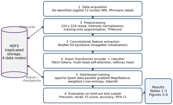
Figure 1: Workflow of the distributed CNN+ViT framework for lumbar disc degeneration classification. The six numbered stages correspond to Protocol sections 1-7: acquisition of de-identified sagittal T2-weighted lumbar spine MRI with Pfirrmann labels; preprocessing (224 x 224 resizing, intensity normalization, training-only augmentation, TFRecord serialization); convolutional feature extraction with a ResNet-50 backbone; Vision Transformer (ViT) encoding and softmax classification; data-parallel training with Apache Spark using Map/Reduce gradient aggregation, weighted cross-entropy, and AdamW; and evaluation on the held-out test subset. The Hadoop Distributed File System (HDFS) stores the serialized records, training shards, and checkpoints across four data nodes. Abbreviations: CNN = convolutional neural network; CI = confidence interval. Please click here to view a larger version of this figure.

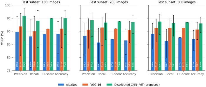
Figure 2: Classification performance of the three models on test subsets of 100, 200, and 300 slices. Precision, recall, F1-score, and accuracy (%) for AlexNet, VGG-16, and the proposed distributed CNN+ViT framework, computed from the confusion-matrix counts in Table 1 with degenerated as the positive class. Error bars are Wilson 95% confidence intervals of the corresponding proportion (n = 100, 200, or 300 slices for accuracy; n = predicted positives for precision; n = reference positives for recall). The F1-score is a harmonic mean and carries no interval. All models were trained under the identical protocol of step 7.4; results are from one training run per model with a fixed random seed. Please click here to view a larger version of this figure.

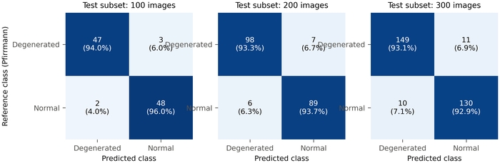
Figure 3: Confusion matrices of the proposed distributed CNN+ViT framework. Rows give the reference class from Pfirrmann grading and columns the predicted class, for the 100-, 200-, and 300-slice test subsets. Each cell shows the count and, in parentheses, the percentage of the row (recall for the degenerated row, specificity for the normal row). Cell shading is proportional to the row percentage. Please click here to view a larger version of this figure.

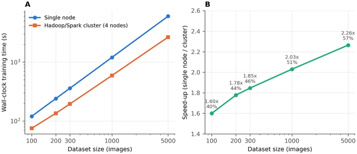
Figure 4: Scalability of the distributed configuration. (A) End-to-end wall-clock training time on a single node and on the four-node Hadoop/Spark cluster at dataset sizes of 100 to 5,000 images (both axes logarithmic). (B) Speed-up (single-node time divided by cluster time) with parallel efficiency (speed-up divided by four nodes) annotated at each point. Each point is a single timed run; times include initialization, data communication, synchronization, and checkpointing overhead. Please click here to view a larger version of this figure.

Table 1: Confusion-matrix counts by model and test-subset size. Number of degenerated and normal slices in each test subset and the true positives (TP), false positives (FP), false negatives (FN), and true negatives (TN) recorded for each model, with degenerated as the positive class. These counts are the primary data used to calculate Table 3, Figure 2, and Figure 3. Please click here to download this Table.

Table 2: Scalability of the distributed configuration. Wall-clock training time, throughput, speed-up, and parallel efficiency for the single-node and four-node configurations at each evaluated dataset size. Please click here to download this Table.

Table 3: Classification performance by model and test-subset size. Precision, recall, specificity, F1-score, and accuracy (%), with Wilson 95% confidence intervals for precision, recall, and accuracy, computed from the counts in Table 1 for AlexNet, VGG-16, and the proposed distributed CNN+ViT framework on test subsets of 100, 200, and 300 slices. Please click here to download this Table.

Supplementary File 1: Data supporting the findings of this study. Please click here to download this file.

Discussion

Critical steps within the protocol

Three steps affect the reliability of the result. First, the data must be partitioned at the patient level rather than the slice level (step 1.3), because slice-level splitting places images from the same patient in more than one subset and inflates every reported metric. Second, the label scheme must be defined once and applied identically to all subsets (step 1.2). Third, augmentation must be confined to the training subset (step 2.3). Where the classes are imbalanced, the weighted objective of Eq. (7) prevents the model from defaulting to the majority class, and fixing the operating threshold on the validation subset (step 7.1) keeps the test estimate unbiased. Reporting the confusion-matrix counts (step 7.2) rather than only derived percentages allows any reader to recompute and check the metrics.

Modifications and troubleshooting

If validation performance is high but test performance is poor, check first for patient-level leakage (step 1.4) and then for augmentation inadvertently applied to the evaluation subsets. If the training loss diverges, reduce the initial learning rate and confirm that intensity normalization is applied before batching. If reported metrics cannot be reproduced from the confusion-matrix counts, the threshold has usually been changed after evaluation or the positive class has been swapped; both are detectable from the per-slice prediction log of Supplemental File 1. If distributed training is slower than single-node training on small datasets, this is the expected behavior: coordination and communication overhead outweighs the parallel benefit until the dataset is large enough, which is why the scaling measurement of step 9.2 is reported across several dataset sizes. The backbone can be replaced by any convolutional network that exposes a spatial feature map; the patch size in step 5.1 must then be adjusted to the new map dimensions.

Significance compared with existing methods

The framework was compared with AlexNet and VGG-16 under an identical protocol and outperformed both on every reported metric at every test-subset size. Because the two baselines differ from one another in depth, the further improvement achieved by the proposed framework supports the interpretation that local-global feature fusion, rather than depth alone, accounts for the difference. This is consistent with reported hybrid CNN-transformer results for lumbar MRI^20,21. The distributed layer is an engineering component that determines the data volume the pipeline can process; it is not a modeling advance, and it is reported as such, with its measured speed-up and efficiency.

Generalizability and external validity

The performance reported here came from data drawn from a single source, and several factors would be expected to affect performance on external data. Scanner vendor and field strength alter signal intensity and contrast, and because Pfirrmann grading depends directly on T2 signal, a shift in intensity distribution translates into a shift in the decision boundary. Acquisition protocol (echo time, repetition time, slice thickness, in-plane resolution, and the choice of sagittal plane) changes the apparent size and sharpness of the disc, and resizing to a fixed 224 x 224 input does not remove this variation. Patient demographics matter because disc desiccation increases with age, so a cohort with a different age distribution shifts the boundary between normal age-related change and early degeneration. Finally, disease prevalence in the target population differs from the prevalence in the training data, and because precision depends on prevalence while sensitivity and specificity do not, the precision reported here would not be expected to transfer unchanged to a population with a different case mix. Domain adaptation, intensity harmonization, and threshold recalibration on local data are the appropriate mitigations. For these reasons, independent external validation on multicenter datasets, acquired on different scanners and reported against reference grading by more than one radiologist, is a prerequisite for any clinical deployment. The present study is a retrospective methodological evaluation and does not establish clinical utility.

Limitations

The demonstrated task is binary detection; multiclass ordinal Pfirrmann grading is an extension rather than a current result. Results are from a single training run per model, and the confidence intervals of the three models overlap, so the observed differences are consistent in direction but not established as statistically significant; repeated runs with different seeds and a larger test cohort are required. Comparison is restricted to AlexNet and VGG-16, and benchmarking against EfficientNet, ConvNeXt, a pure ViT, and Swin Transformer remains to be performed. Per-case attribution maps were not evaluated. The ViT encoder increases computational and memory cost relative to lightweight convolutional networks, which may constrain deployment in resource-limited centers. Evaluation was performed on data from a single source, and no external or multicenter validation was undertaken. The benefit of the distributed layer is realized only at scale and adds coordination overhead on small datasets.

Future applications

The elements below are anticipated directions and were not evaluated in this study. They include extension to multiclass Pfirrmann grading with ordinal metrics; per-case attribution with gradient-weighted class activation mapping³⁰ using Supplemental File 1; multicenter external validation; multimodal fusion of MRI with CT and with structured clinical data; federated training across institutions to improve generalization without transferring patient data; and integration with validation and certification frameworks for clinical artificial intelligence³¹.

Matériaux

Liste des matériaux utilisés dans cet article

Nom	Entreprise	Numéro de catalogue	Commentaires
Apache Hadoop	Apache Software Foundation	Version 3.3.4	Distributed file system (HDFS) and cluster resource management; open source
Apache Spark / PySpark	Apache Software Foundation	Version 3.4.0	Distributed data loading and data-parallel training; open source
CUDA Toolkit	NVIDIA	Version 11.8	GPU compute platform used by TensorFlow
cuDNN	NVIDIA	Version 8.6	GPU-accelerated deep learning primitives
Gigabit Ethernet switch	Generic	10 GbE	Interconnect between cluster nodes
GPU accelerator	NVIDIA	Tesla V100, 32 GB	One GPU per compute node, four nodes
NumPy	NumPy developers	Version 1.24	Numerical arrays; open source
pydicom	pydicom developers	Version 2.4	DICOM reading and header de-identification; open source
Python	Python Software Foundation	Version 3.10	Programming language; open source
scikit-learn	scikit-learn developers	Version 1.3	Patient-level stratified splitting and confusion-matrix metrics; open source
Server node	Generic	Intel Xeon Gold 6248R, 64 GB RAM, 2 TB NVMe SSD	Four identical nodes; one used for the single-node baseline
TensorFlow / Keras	Google	Version 2.12	Model definition, training and TFRecord serialization; open source
TensorFlow Serving	Google	Version 2.12	REST inference endpoint for single-case prediction; open source
Ubuntu Linux	Canonical	Version 22.04 LTS	Operating system on all nodes