Cette étude présente un protocole reproductible permettant d'optimiser la disposition d'expositions immersives en combinant un recuit simulé adaptatif, une sélection de propositions dépendante des étapes et une régulation de réchauffage. La disposition retenue a été mise en œuvre dans un environnement d'exposition en réalité virtuelle et évaluée à l'aide de métriques de coût spatial, de journaux comportementaux des participants et de notes attribuées après l'expérience.
Un abonnement JoVE est requis pour visualiser ce contenu. Connectez-vous ou commencez votre période d'essai gratuite.
Article de recherche
Optimisation de la conception d'espaces d'exposition immersifs à l'aide du recuit simulé adaptatif avec réchauffement et d'une évaluation en réalité virtuelle
Dans cet article
Résumé
Résumé
Les espaces d'exposition immersifs nécessitent des agencements favorisant une circulation efficace, un guidage clair, une interaction équilibrée et un confort environnemental optimal. Toutefois, les agencements d'exposition sont souvent conçus manuellement, ce qui rend difficile l'évaluation simultanée de la longueur des parcours, de l'accessibilité visuelle, du risque d'agglomération, du confort environnemental et de la répartition des nœuds d'interaction. Cette étude a mis au point et évalué un flux de travail d'optimisation de conception spatiale fondé sur un recuit simulé adaptatif avec sélection de propositions dépendante des étapes et contrôle de réchauffage. Une salle d'exposition immersive de 36 m × 24 m a été conçue comprenant six zones thématiques, des couloirs de transition, une aire de repos et plusieurs nœuds d'interaction. Trois conditions d'agencement ont été comparées : agencement manuel, agencement par recuit simulé standard et agencement par recuit simulé adaptatif avec réchauffage. Le modèle d'optimisation a minimisé une fonction de coût spatial pondéré intégrant la distance parcourue, l'accessibilité visuelle, l'affluence, le confort environnemental et l'équilibre d'interaction. Les agencements retenus ont été implémentés dans des scènes d'exposition en réalité virtuelle et évalués à partir des journaux comportementaux des participants et des évaluations post-expérience. L'algorithme adaptatif a produit un coût spatial final plus faible, un pourcentage d'amélioration plus élevé et un nombre réduit d'itérations vers la meilleure solution par rapport au recuit simulé standard, avec une augmentation modeste du temps de calcul. Les participants affectés à l'agencement adaptatif ont signalé une satisfaction plus élevée, une sensation de présence plus marquée, un guidage plus clair, une impression d'affluence moindre et une charge cognitive réduite ; ils ont également parcouru l'itinéraire avec une distance de marche plus courte, moins d'hésitations, un temps d'arrêt plus long et une couverture plus étendue sur la carte thermique. Ces résultats valident le flux de travail comme outil d'aide à la décision pour le scénario d'exposition testé ; ils n'établissent toutefois pas un agencement d'exposition universellement optimal ni une supériorité sur toutes les métaheuristiques alternatives.
Introduction
Les espaces d'exposition immersifs combinent de plus en plus la conception spatiale, les médias numériques, les écrans interactifs et les technologies de réalité virtuelle afin de créer des environnements dans lesquels les visiteurs n'observent pas simplement le contenu, mais s'y déplacent, y réagissent et interprètent l'exposition comme une expérience spatiale. Dans de tels contextes, la qualité de l'expérience dépend non seulement de la richesse du contenu visuel ou interactif, mais aussi de la continuité des parcours, de la visibilité, de l'affluence, du confort environnemental et de la répartition des possibilités d'interaction. La conception des espaces d'exposition implique donc un problème à variables multiples : une agencement doit guider les visiteurs de manière efficace tout en préservant la séquence narrative, l'ouverture perceptive et les opportunités d'engagement. Les études sur le comportement dans les musées et les expositions ont depuis longtemps montré que l'expérience des visiteurs est façonnée par l'organisation spatiale, la structure de la circulation et l'accessibilité interprétative, et non pas uniquement par le contenu des expositions1.
La théorie de la configuration spatiale fournit une base utile pour traiter l'agencement d'une exposition comme un problème de conception pouvant être analysé. Selon cette perspective, l'espace n'est pas un contenant passif pour des objets ; il organise le déplacement, la rencontre, la visibilité et le choix. La configuration architecturale peut influencer la manière dont les personnes se déplacent dans un environnement et la facilité avec laquelle elles comprennent les relations entre les espaces2. L'analyse spatiale fondée sur la visibilité appuie davantage ce point de vue en montrant que les champs visuels et les relations de ligne de mire peuvent être modélisés comme des caractéristiques mesurables de la cognition spatiale et de la navigation3. Ces idées sont particulièrement pertinentes pour les expositions immersives, car les visiteurs doivent continuellement intégrer des informations visuelles, des décisions d'itinéraire, des indices d'interaction et des stimuli environnementaux lorsqu'ils se déplacent dans l'exposition.
Parallèlement, les technologies immersives ont élargi les possibilités de conception et de test des environnements d'exposition avant leur mise en œuvre physique. Les interfaces virtuelles et immersives permettent aux chercheurs et aux concepteurs d'analyser la manière dont les utilisateurs perçoivent et se comportent dans des conditions spatiales contrôlées, ce qui permet de comparer différentes configurations tout en maintenant constants le contenu et les paramètres environnementaux4. Les revues sur les applications de réalité virtuelle immersive montrent que la structure spatiale, la conception de l'interaction et la clarté des tâches sont des facteurs déterminants importants de l'engagement des utilisateurs et de la qualité de l'apprentissage5. Des preuves issues de méta-analyses suggèrent également que le niveau et le type d'immersion peuvent influencer le sentiment de présence, mais que l'immersion seule ne garantit pas de meilleurs résultats si l'environnement est mal organisé ou difficile à naviguer6.
L'expérience utilisateur d'une exposition immersive est étroitement liée à la présence, à la charge cognitive et au confort physique. La présence reflète dans quelle mesure les utilisateurs ont l'impression de se trouver dans un environnement médiatisé, ce qui en fait un résultat clé dans les environnements virtuels et immersifs7. Toutefois, les environnements immersifs peuvent également induire une charge cognitive lorsque la navigation, l'interaction ou l'information sensorielle ne sont pas bien coordonnées8. Pour cette raison, l'optimisation de l'espace d'exposition ne devrait pas seulement accroître la densité d'interactions ou la stimulation visuelle. Elle devrait favoriser une expérience spatiale cohérente, réduire les décisions inutiles concernant les trajets et minimiser la fatigue évitable. Les symptômes de mal des simulateurs doivent également être surveillés, car l'inconfort peut affecter à la fois la sécurité de l'exposition à la réalité virtuelle et l'interprétation des résultats relatifs à l'expérience utilisateur9.
Malgré ces exigences, de nombreux aménagements d'exposition sont encore conçus à partir de l'expérience des concepteurs, d'ajustements manuels itératifs ou d'observations a posteriori des visiteurs. Ces approches restent pertinentes, mais elles rendent difficile l'évaluation simultanée de plusieurs contraintes de disposition. La conception spatiale d'expositions immersives peut être formulée comme un problème d'optimisation sous contraintes prenant en compte conjointement la longueur des parcours, la visibilité, l'affluence, le confort et la répartition des interactions. Le recuit simulé convient à ce type de problème, car il permet d'explorer des espaces de solutions vastes et irréguliers tout en autorisant l'acceptation contrôlée de solutions intermédiaires non améliorantes, aidant ainsi à sortir des optima locaux10. Sa logique d'acceptation suit la règle de Metropolis11, tandis que le cadre plus général de Metropolis-Hastings introduit un rapport entre les densités de proposition directe et inverse lorsque le noyau de proposition est asymétrique12. Dans la mise en œuvre actuelle, les quatre noyaux de proposition conditionnels sont symétriques ; par conséquent, la dérivation formelle montre que le rapport de Hastings vaut un pour les mouvements faisables réversibles. La méthode est donc décrite comme un recuit simulé adaptatif avec acceptation selon Metropolis et réchauffage, plutôt que comme un échantillonneur Metropolis-Hastings distinct.
Depuis longtemps, les variantes du recuit simulé adaptatif utilisent une sélection non uniforme des voisinages, la modification du protocole de refroidissement, le réchauffage, les stratégies de redémarrage et des composants de recherche hybrides13,14. La présente implémentation doit donc être considérée comme une configuration spécifique à l'application, et non comme une nouvelle primitive métaheuristique. Sa contribution réside dans le couplage explicite d'un calendrier de propositions à quatre mouvements dépendant de l'étape et du réchauffage avec des contraintes de faisabilité spécifiques à l'exposition, une fonction de coût spatial transparente à composants multiples, et une validation en réalité virtuelle au niveau des participants15. Cette position plus restreinte distingue clairement le présent flux de travail des affirmations relatives à un principe d'optimisation fondamentalement nouveau. On s'attendait à ce que la sélection des propositions dépendant de l'étape oriente la recherche, passant d'une exploration plus large des séquences/voies vers un affinement spatial local, tandis que le réchauffage restaurait la mobilité de la recherche après une stagnation. On s'attendait à ce que cet équilibre entre exploration et exploitation réduise le piégeage prématuré dans des minima locaux et augmente la probabilité d'atteindre une configuration réalisable à coût plus faible dans un budget d'itérations nominal identique.
Cette étude propose un flux de travail reproductible qui intègre un recuit simulé adaptatif, une sélection de propositions dépendante des étapes, un contrôle de réchauffage, un modèle de coût spatial à composantes multiples et une évaluation en réalité virtuelle au niveau des participants. La contribution méthodologique est orientée vers l'application et axée sur la reproductibilité, plutôt que sur l'affirmation d'un principe d'optimisation fondamentalement nouveau16. La méthode compare une disposition manuelle, une disposition issue d'un recuit simulé standard et une disposition issue d'un recuit simulé adaptatif avec réchauffage, dans un environnement d'exposition en réalité virtuelle contrôlé. L'étude examine à la fois les résultats algorithmiques et les résultats au niveau des participants, notamment le coût spatial final, le pourcentage d'amélioration, le sentiment de présence, la clarté de l'orientation, la satisfaction, la charge cognitive, la distance parcourue, le nombre d'hésitations, le temps d'immobilisation et la couverture des cartes thermiques. L'hypothèse principale était que la méthode adaptative permettrait d'obtenir un coût spatial final inférieur à celui du recuit simulé standard ; au niveau des participants, la disposition correspondante devait améliorer la satisfaction générale et l'efficacité de parcours par rapport aux dispositions manuelle et issue du recuit simulé standard. Ce cadre suit la logique plus large des méthodes de conception métaheuristiques, dans lesquelles la recherche computationnelle soutient le jugement humain en matière de conception sans le remplacer17.
Accès restreint. Veuillez vous connecter ou commencer un essai pour afficher ce contenu.
Protocole
The study protocol was reviewed by Henan Agricultural University and was determined to be exempt from formal ethics review on December 20, 2025. No separate ethics approval or exemption reference number was issued by the reviewing body. Written informed consent was obtained from all participants before enrollment.
Participant preparation
Adult participants aged 18–60 years with normal or corrected-to-normal vision were recruited. Participants who reported severe vestibular disorders, uncontrolled epilepsy, severe visual impairment, recent major surgery, or previous serious discomfort during virtual-reality exposure were excluded. Each participant completed a screening form before the experiment. Age group, gender, education level, prior virtual-reality experience, and prior museum or exhibition-visiting frequency were recorded as control variables.
Participants were assigned to one of three layout conditions using a computer-generated randomization list: manual layout, standard simulated annealing layout, or adaptive simulated annealing with reheating layout. A between-subject design was used to avoid learning effects across layouts. The allocation ratio was set to 1:1:1, with 60 participants assigned to each condition and 180 participants in total. Age group, gender, education level, previous virtual-reality experience, and museum/exhibition-visiting frequency were recorded before allocation for descriptive assessment of participant characteristics; these variables were not used as post-randomization exclusion criteria.
Exhibition-space model preparation
A rectangular immersive exhibition hall measuring 36 m x 24 m with a ceiling height of 4.5 m was constructed. The total usable floor area was set to 864 m2. One entrance and one exit were placed on opposite short sides of the hall. Both the entrance and exit widths were set to 3.0 m and were kept fixed across all layout conditions.
The exhibition hall was divided into six thematic exhibition zones, two transition corridors, one rest area, and one main visitor route. The allowable area for each thematic zone was set to 80–130 m2, and the rest-area allocation was set to 40 m2. The allowable main-pathway width was set to 1.8–3.5 m. Eight to twelve interaction nodes were placed in each layout. Each interaction node was defined as a point where participants could stop, activate digital content, view an exhibit, or change direction.
The floor plan was discretized into 0.5 m x 0.5 m grid cells. The grid was used for visibility analysis, route-continuity checking, heatmap coverage calculation, and local density estimation. Each thematic zone was represented by its center coordinate, boundary polygon, area, and route-sequence position. Each interaction node was represented by its coordinate, associated zone, trigger radius, and clearance area.
Spatial configuration was treated as the core design variable because exhibition layout, visibility, and route structure affect visitor movement, wayfinding, and spatial cognition18. The complete workflow, from spatial model construction to layout optimization, virtual-scene implementation, participant testing, and statistical analysis, is shown in Figure 1.
Layout parameters and feasibility constraints
The same feasibility constraints were applied to all layout conditions. First, all thematic zones were required to remain inside the 36 m x 24 m boundary. Second, thematic zones were not allowed to overlap. Third, the main visitor route was required to connect the entrance, six thematic zones, a rest area, and the exit without interruption. Fourth, interaction nodes were not allowed to block the main path. Fifth, each interaction node was required to retain a clearance radius of at least 1.2 m. Sixth, the predicted local density on the main route was required to be no more than 1.50 persons/m2. Seventh, the final route was required to contain no dead ends or disconnected subpaths.
The same scene scale, route rules, environmental targets, and interaction settings were used across the three layout conditions. Before the optimization algorithms were run, the hall dimensions, functional-zone parameters, pathway-width range, interaction-node settings, feasibility thresholds, virtual-reality settings, objective-function weights, algorithm parameters, and outcome definitions were recorded. These parameters defined the reproducible boundary of the protocol and are summarized in Table 1.
Spatial-cost function
Each candidate layout was evaluated using the weighted spatial-cost function:

where F(x) is the total spatial cost of layout x. Cdistance(x) is the walking-distance cost, Cvisibility(x) is the visual-accessibility cost, Ccrowding(x) is the crowding cost, Ccomfort(x) is the environmental-comfort penalty, and Cinteraction(x) is the interaction-balance penalty. A lower F(x) indicates a more favorable layout.
The walking-distance cost was calculated as:

where Lx is the total route length of layout x in meters. A reference maximum route length of 120 m was used.
The visual-accessibility cost was calculated as:
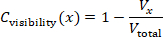
where Vx is the thematic-zone frontage visible from the main route, and Vtotal is the total frontage length of all thematic zones. Line-of-sight rays were emitted every 0.5 m along the visitor route. Exhibition partitions, walls, and zone boundaries were treated as occluding objects.
The crowding cost was calculated as:
Ccrowding(x) = min(Dmax / 1.50, 1)
where Dmax is the maximum predicted local density in persons/m2. An upper density threshold of 1.50 persons/m2 was used for the main route.
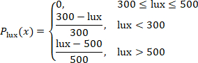
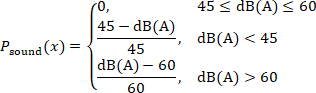
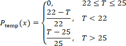
The environmental-comfort penalty was calculated as:

The illuminance penalty was set as:
The sound-pressure penalty was set as:
The carbon dioxide penalty was set as:

The temperature penalty was set as:
The interaction-balance penalty was calculated as:

where sk is the route distance between two adjacent interaction nodes. A lower value indicates a more even distribution of interaction opportunities along the visitor route.
Environmental comfort is included because lighting, sound, air quality, and temperature influence fatigue, comfort, and willingness to remain in exhibition environments19. The environmental ranges are protocol control targets rather than universal regulatory limits. The 300–500 lx illuminance band is consistent with current Chinese building and museum-lighting guidance; the carbon-dioxide target of <900 ppm is deliberately more conservative than the 1,000 ppm daily-average limit in GB/T 18883-202220,21; the 22–25 °C temperature band is within commonly accepted thermal-comfort conditions for lightly active occupants22; and 45–60 dB(A) is used as a controlled ambient-sound band rather than as a statutory indoor-noise limit23,24.
The objective-function weights were selected as explicit, scenario-specific design priorities rather than as universal coefficients or preference estimates fitted from participant outcomes. Walking distance and crowding each received a weight of 0.25 because route efficiency and congestion control were treated as the two primary operational constraints; visual accessibility received 0.20 because visibility affects orientation and exhibits exposure; environmental comfort and interaction each received 0.15 so that these factors influence the search without dominating circulation-related terms. Because exhibition priorities can differ by context, the protocol tests local weight robustness by perturbing each weight by ±10% individually and proportionally renormalizing the remaining weights so that the total remains 1.00. The resulting coefficients should therefore be interpreted as protocol-specific design settings that can be recalibrated for artistic, historical, scientific, or commercial exhibitions.
Manual layout generation
The manual layout was created as the baseline condition. The six thematic zones were arranged in a conventional narrative sequence from entrance to exit. The rest area was placed near the middle section of the route. The initial main-pathway width was set to 2.2 m. Interaction nodes were placed near the entrance of each thematic zone and at major route-turning points. The manual layout was checked against all feasibility constraints. Zone boundaries were adjusted only when a constraint was violated. After the layout became feasible, total route length, visible frontage ratio, maximum local density, environmental-comfort penalty, interaction-spacing coefficient, and total spatial cost were recorded.
Standard simulated annealing
The feasible manual layout was used as the initial state. The initial temperature was set to 100, the cooling coefficient to 0.95, the maximum number of iterations to 1,500, and the stagnation threshold to 200 iterations. The algorithm was run with 30 independent random seeds. These values were operational protocol settings used to define a matched computational budget; they were not presented as literature-derived universal constants or outcome-tuned optima. T₀ = 100 permitted broad early exploration, α = 0.95 provided gradual cooling, 1,500 iterations provided each run with the same upper search budget, and the 200-iteration stagnation threshold prevented prolonged continuation after no improvement. The same temperature and maximum-iteration settings were used for the adaptive method so that differences were attributable to proposal scheduling and reheating rather than to a larger nominal search budget.
At each iteration, one neighboring layout was generated by applying one move: moving one thematic zone by 0.5–2.0 m, swapping the sequence positions of two thematic zones, adjusting one pathway segment by 0.1–0.3 m, or moving one interaction node by 0.5–1.5 m. A proposed layout was rejected immediately if it violated any feasibility constraint.
If the proposed layout was feasible and had a lower spatial cost, it was accepted. If it had a higher spatial cost, it was accepted according to the probability equation:
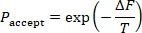
where ΔF is the increase in spatial cost, and T is the current temperature. The temperature after each iteration was updated using:
Tnew = 0.95Told
Each run was stopped when the maximum iteration count was reached or when the best spatial cost did not improve for 200 consecutive iterations. Simulated annealing was considered suitable for this task because exhibition layout optimization is a combinatorial spatial problem that cannot be solved efficiently by exhaustive search.
Standard simulated annealing was used as the primary numerical algorithmic benchmark because it shared the same layout encoding, feasibility rules, objective function, initialization, temperature schedule, and computational budget as the adaptive condition. Standard simulated annealing was the sole numerical metaheuristic comparator in this study and therefore functioned as a matched ablation-like baseline for the added proposal scheduling and reheating at the workflow level. Genetic algorithms, particle swarm optimization, ant colony optimization, and learning-based optimizers were not part of the experiment; accordingly, performance claims were restricted to the matched standard-SA baseline. For each run, the random seed, initial spatial cost, final spatial cost, improvement percentage, number of iterations to the best solution, runtime, acceptance rate, and feasibility status were stored. Improvement percentage was calculated using the equation:

Adaptive simulated annealing with reheating
The same initial layout, feasibility constraints, initial temperature, cooling coefficient, maximum iteration count, and 30 random seeds as the standard simulated annealing condition were used. The adaptive algorithm differed only in its stage-dependent move-class probabilities and reheating rule, while retaining the standard Metropolis acceptance rule for feasible candidate layouts. Four proposal move classes were defined: local displacement (L), zone-sequence swap (S), pathway-width adjustment (W), and interaction-node relocation (N). During the first 40% of iterations, the move-class probabilities were set to pL = 0.20, pS = 0.35, pW = 0.30, and pN = 0.15. During the final 60%, they were set to pL = 0.35, pS = 0.15, pW = 0.20, and pN = 0.30. This change in move-class frequency shifted the search from broader sequence/pathway exploration toward local spatial refinement and adjustment of interaction nodes.
At iteration t, the full proposal density was expressed as q(x′|x,t) = pm(t)qm(x′|x), where m ∈ {L,S,W,N} represented the selected move class and pm(t) represented its phase-specific probability. For local displacement, one of six thematic zones was selected uniformly, a displacement direction was drawn uniformly on [0,2π), and a displacement magnitude was drawn uniformly on [0.5,2.0] m; therefore, qL was proportional to (1/6)(1/2π)(1/1.5). For a zone-sequence swap, one of the 15 unordered zone pairs was selected uniformly, giving qS = 1/15. For pathway-width adjustment, one of J adjustable pathway segments was selected uniformly, and a signed change was drawn uniformly from [−0.3,−0.1] ∪ [0.1,0.3] m, giving qW = (1/J)(1/0.4). For interaction-node relocation, one of K current interaction nodes was selected uniformly, a direction was drawn uniformly on [0,2π), and a displacement magnitude was drawn uniformly on [0.5,1.5] m, giving qN proportional to (1/K)(1/2π)(1/1.0). Constraint-violating proposals were rejected and contributed a self-transition.

For every reversible feasible move in this implementation, the conditional proposal kernel was symmetric: qm(x′|x) = qm(x|x′). Because the same phase-specific move-class probability pm(t) was applied to the forward and reverse transition at a given iteration, q(x|x′,t)/q(x′|x,t) = 1. The acceptance probability, therefore, is reduced to the standard simulated-annealing Metropolis rule, A(x→x′) = min{1, exp[−(C(x′)−C(x))/T]}. No non-trivial Hastings correction was applied; the method is therefore termed adaptive simulated annealing with reheating rather than a Metropolis-Hastings sampler25.
Reheating was applied when the best spatial cost did not improve for 150 consecutive iterations, thereby intentionally intervening before the 200-iteration stagnation stop used in standard simulated annealing. The current temperature was increased by 10%, and up to 3 reheating events were allowed per run. The same algorithm-performance variables as in the standard simulated annealing condition were stored. The experiment evaluated the combined stage-dependent proposal schedule plus reheating configuration and therefore did not estimate the independent causal contribution of each component. Stepwise pseudocode for the exact proposal, feasibility, Metropolis acceptance, temperature update, reheating, and output storage sequence was provided in Supplementary File 3.
Treheated = 1.10Tcurrent
Final layouts
One final layout was selected for each condition. The feasible manual layout was used for the manual condition. Under the standard simulated annealing conditions, the run with the lowest final spatial cost among the 30 runs was selected. For the adaptive simulated annealing with reheating condition, the feasible run with the lowest final spatial cost among the 30 runs was selected. Before the selected layouts were exported, a final feasibility check confirmed that all zones were inside the boundary, no zones overlapped, the route was continuous, the entrance and exit were unchanged, interaction-node clearance was at least 1.2 m, maximum density remained below 1.50 persons/m2, and all thematic zones were reachable from the main route.
Virtual exhibition scenes
Three virtual exhibition scenes were built in Unity 2022.3.22f1 LTS (Unity Technologies) using XR Interaction Toolkit 2.5.4. The scenes were presented through a Meta Quest 2 head-mounted display (Meta Platforms) using six-degree-of-freedom head and controller tracking. Exhibition content, visual style, object models, signage style, lighting assets, ambient sound, interaction mechanism, and navigation instructions were kept identical across the three scenes. Only spatial arrangement, route sequence, pathway width, and interaction-node placement varied.
The virtual camera height was set to 1.65 m, and the walking speed was set to 1.2 m/s. Teleportation was disabled. The same starting trigger at the entrance and the same completion trigger at the exit were used. The interaction-node trigger radius was set to 1.0 m. Whether each interaction node was visited was recorded.
The same six thematic contents were used in all scenes. Each theme was assigned to its corresponding zone, regardless of layout conditions. Wall height, partition style, media display size, text density, and exhibit object scale were kept constant. Virtual-reality environments were considered appropriate for this protocol because they enabled the examination of spatial presence, route clarity, and visitor experience under controlled layout conditions26.
The hardware, software, environmental-monitoring tools, questionnaire/codebook files, and analysis resources required to reproduce the protocol were listed in the Table of Materials and organized as Supplementary Files 1–3. Research resources with registered Research Resource Identifiers (RRIDs) were listed by RRID in the Table of Materials.
Participant session
One participant was tested at a time. The participant sat for 2 min before the session. The head-mounted display was fitted, and the interpupillary distance was adjusted according to the participant's comfort. A 2 min practice scene that was not part of the exhibition was provided. The practice scene was used only to familiarize the participant with movement and interaction.
Because one participant was tested at a time, crowding in the protocol was represented by model-based density estimates rather than emergent simultaneous group movement. Multi-user co-presence, interpersonal avoidance, and dynamic crowd interactions were therefore not directly simulated and were considered when interpreting crowd-related outcomes.
After practice, the assigned exhibition scene was started. The participant was instructed to enter the exhibition, follow the route naturally, interact with marked nodes, and exit after completing all six thematic zones. Additional route guidance was provided only if the participant could not proceed for more than 30 s. Completion time, dwell time, walking distance, hesitation count, interaction-node visits, and trajectory coordinates were recorded automatically.
The session ended when the participant reached the exit trigger. The head-mounted display was removed, and the participant was allowed to rest for 3 min. The participant completed the post-experience questionnaire immediately after the rest period.
Behavioral, environmental, and questionnaire outcomes
Completion time was defined as the time from entrance-trigger activation to exit-trigger activation. Dwell time was defined as the total time spent inside thematic zones and interaction-node areas. Walking distance was defined as cumulative path length from trajectory coordinates. Hesitation count was defined as the number of pauses longer than 3 s outside interaction-node areas. Heatmap coverage was calculated using:

Average illuminance was recorded using a Testo 540 illuminance meter (Testo SE & Co. KGaA), sound pressure level using a Testo 816-1 Class 2 sound level meter (Testo SE & Co. KGaA), carbon-dioxide concentration using a Testo 535 CO₂ measuring instrument (Testo SE & Co. KGaA), and ambient temperature using a Testo 605i thermohygrometer (Testo SE & Co. KGaA). The same monitoring positions were used across the three scene conditions. Illuminance was recorded in lx, sound pressure level in dB(A), carbon dioxide in ppm, and temperature in °C.
Presence and spatial-presence domains were measured using the 7-point scoring structure specified in the study protocol. These constructs were interpreted with reference to the validated Presence Questionnaire (PQ) framework of Witmer and Singer and the Igroup Presence Questionnaire (IPQ) framework of Schubert et al.27. The study variables were reported as domain-level 7-point scores rather than as standard PQ or IPQ total scores. For simulator sickness, the Simulator Sickness Questionnaire symptom framework was used together with the prespecified 0–30 study summary variable; higher values indicated greater discomfort. This 0–30 study summary was reported separately from the standard weighted SSQ Total Severity score, consistent with the distinction between simulator-sickness measurement conventions and cybersickness reporting28. Interaction quality, wayfinding clarity, visual comfort, acoustic comfort, thermal comfort, perceived crowding, cognitive load, and overall satisfaction were measured using the study-specific, multi-item, 7-point rating scales. Supplementary File 2 documented the construct source, score range, and reporting convention for each domain.
Study outcomes
The primary algorithmic outcome was defined as the final spatial cost. The primary visitor-experience outcome was defined as overall satisfaction. Secondary algorithmic outcomes were defined as the improvement percentage, the number of iterations to the best solution, the runtime, and the acceptance rate. Secondary visitor-experience outcomes were defined as presence, spatial presence, interaction quality, wayfinding clarity, visual comfort, acoustic comfort, thermal comfort, perceived crowding, cognitive load, simulator sickness, completion time, dwell time, walking distance, hesitation count, and heatmap coverage. Completion time and walking distance were used to evaluate route efficiency. Hesitation count and wayfinding clarity were used to evaluate navigation quality. Presence, spatial presence, interaction quality, and dwell time were used to evaluate immersive engagement. Perceived crowding, cognitive load, comfort ratings, and simulator sickness were used to evaluate experiential burden.
Data cleaning and quality control
All participant records were checked before analysis. It was confirmed that each record had a single participant identifier, a single condition label, complete behavioral logs and questionnaire scores, and no duplicate identifiers. Presence, spatial-presence, and study-specific experience ratings were restricted to their defined 1–7 ranges. The simulator-sickness study summary variable was restricted to its prespecified 0–30 range. The questionnaire/codebook file was checked to confirm that it documented the construct source, response range, domain construction, and derived-score definitions used in the analysis.
A participant record was excluded if the session was not completed, completion time was less than 3 min or greater than 25 min, heatmap coverage was less than 10%, the trajectory log was incomplete or technically invalid, walking distance was less than 20 m in conjunction with an incomplete/invalid trajectory record, or the participant requested early termination. No upper walking-distance cutoff was applied; walking distance was retained as a continuous study outcome across its valid observed range. An algorithm run was excluded from layout selection if it violated any feasibility constraint. Random seeds, layout files, algorithm outputs, questionnaire/codebook files, and analysis scripts were preserved for reproducibility. Random-seed preservation was necessary because stochastic optimization outputs could vary with initialization and proposal behavior29.
Algorithm performance
The 30 standard simulated annealing runs and 30 adaptive simulated annealing with reheating runs were analyzed. Initial spatial cost, final spatial cost, improvement percentage, iterations to best solution, runtime, and acceptance rate were summarized as mean ± standard deviation (SD), and 95% confidence intervals were reported for the group means and between-algorithm differences.
Normality was assessed using quantile-quantile (Q-Q) plots and the Shapiro-Wilk test. Homogeneity of variance was assessed using Levene's test. The two algorithmic conditions were compared using independent-samples t tests when assumptions were met. Mann-Whitney U tests were used when assumptions were not met. Two-sided p values, 95% confidence intervals, and effect sizes were reported. Cohen's d was calculated using the equation

where:

Rank-biserial correlation was used for nonparametric comparisons. Sensitivity analysis was conducted by changing each objective-function weight by ±10% individually and proportionally renormalizing the remaining four weights so that the total remained 1.00. The final spatial cost and improvement percentage were recalculated for each alternative weight vector. The algorithmic comparison was considered stable when the adaptive simulated annealing with reheating condition retained a lower final spatial cost across the alternative weight settings.
Participant outcome analysis
Participant outcomes across the three layout conditions were analyzed using IBM SPSS Statistics 27.0 (IBM Corp.). Continuous variables were reported as mean ± SD, and categorical variables were reported as counts and percentages. Normality was assessed using Q-Q plots and the Shapiro-Wilk test. Homogeneity of variance was assessed using Levene's test. One-way analysis of variance (ANOVA) was used for normally distributed outcomes with acceptable homogeneity of variance. Welch's ANOVA was used when the assumption of homogeneity of variance was violated. Kruskal-Wallis tests were used for non-normal outcomes.
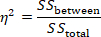
Pairwise comparisons were conducted among the manual layout, standard simulated annealing layout, and adaptive simulated annealing with reheating layout. The three pairwise comparisons within each outcome were adjusted using the Holm method. The 95% confidence intervals were reported together with adjusted p-values. Eta-squared was reported for standard ANOVA, omega-squared for Welch's ANOVA, epsilon-squared for Kruskal-Wallis tests, and standardized mean differences for pairwise comparisons. As a supplementary robustness analysis, pairwise Welch contrasts were calculated from the group mean, SD, and n = 60 per group. Welch degrees of freedom, two-sided p values, Holm-adjusted p values, 95% CIs for mean differences, and Hedges g were calculated. This supplementary analysis used the group-level statistics and was presented in Supplementary Table 1.
The randomized 1:1:1 three-group comparison was treated as the primary analysis. Age group, gender, education level, previous virtual-reality experience, and museum/exhibition-visiting frequency were recorded before allocation to characterize the sample and identify obvious imbalance. The trial was not designed or powered for subgroup interaction tests, and no prespecified moderator model was included; these characteristics were therefore treated as contextual variables rather than demonstrated moderators. Random allocation provided design-based control over baseline characteristics, while the residual influence of prior VR familiarity was explicitly retained as a limitation. Eta-squared was calculated using
Epsilon-squared for Kruskal-Wallis tests was calculated as:
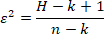
where H is the Kruskal-Wallis test statistic, k is the number of groups, and n is the total sample size.
Overall satisfaction, presence, wayfinding clarity, perceived crowding, cognitive load, completion time, walking distance, hesitation count, and heatmap coverage were prioritized in the interpretation because these variables directly reflected spatial efficiency and immersive visitor experience.
Accès restreint. Veuillez vous connecter ou commencer un essai pour afficher ce contenu.
Résultats
Flux des participants et complétude des données
Un total de 180 participants ont terminé l'expérience d'exposition immersive et ont été inclus dans l'analyse finale. Les trois conditions de disposition étaient équilibrées, avec 60 participants affectés à la disposition manuelle, 60 à la disposition standard par recuit simulé et 60 à la disposition par recuit simulé adaptatif avec réchauffage. Aucun enregistrement de participant n'a été exclu après le contrôle de qualité des données. Tous les journa...
Accès restreint. Veuillez vous connecter ou commencer un essai pour afficher ce contenu.
Discussion
La présente étude a évalué un flux de travail reproductible pour l'aménagement d'expositions, combinant un modèle de coût spatial pondéré, un recuit simulé adaptatif avec réchauffage et des tests auprès de participants en réalité virtuelle. Dans le scénario prédéfini de 36 m x 24 m, l'aménagement adaptatif a permis d'obtenir un coût spatial inférieur à celui du recuit simulé standard et s'est associé à une satisfaction plus élevée, une présence plus marquée, une orientation plus claire, des trajets plus courts, moins d'h...
Accès restreint. Veuillez vous connecter ou commencer un essai pour afficher ce contenu.
Déclarations de divulgation
Les auteurs déclarent ne pas avoir d'intérêts financiers concurrents.
Remerciements
Les auteurs remercient les participants ayant pris part à l'évaluation de l'exposition en réalité virtuelle. Les auteurs remercient également l'École d'art et de design et le Collège des sciences de l'information et de gestion de l'Université agricole du Henan pour leur soutien dans le développement et l'évaluation du flux de travail de conception d'espace d'exposition immersif. L'étude n'a reçu aucun financement externe. Les travaux ont été réalisés grâce aux ressources propres des auteurs et aux installations institutionnelles courantes de l'Université agricole du Henan.
Accès restreint. Veuillez vous connecter ou commencer un essai pour afficher ce contenu.
Matériaux
| Nom | Entreprise | Numéro de catalogue | Commentaires |
|---|---|---|---|
| Logiciel de modélisation 3D | Blender Foundation | N/A | Blender 4.0.2 ; utilisé pour construire la géométrie de l'espace d'exposition, les zones thématiques, les cloisons et les éléments spatiaux. RRID : SCR_008606 |
| Scripts d'analyse | Scripts de recherche personnalisés | N/A | Version 1.0 ; utilisés pour l'analyse statistique, l'analyse de sensibilité, le calcul des intervalles de confiance et la préparation des données des figures. |
| Moniteur de dioxyde de carbone | Testo SE & Co. KGaA | testo 535 ; 0563 0535 | Appareil numérique de mesure du CO2 ; plage de mesure 0–10 000 ppm ; utilisé comme contrôle de protocole de la concentration en dioxyde de carbone selon l'objectif environnemental prédéfini. |
| Station de travail de bureau | Dell Technologies | Precision 3660 Tower | 32 Go de RAM ; utilisée pour le rendu de scènes virtuelles, la simulation de disposition, l'exécution d'algorithmes et l'enregistrement des sessions des participants. |
| Scripts de génération de figures | Scripts de recherche personnalisés | N/A | Version 1.0 ; utilisés pour générer des graphiques de performance des algorithmes, des graphiques des résultats des visiteurs et des cartes thermiques de trajectoires. |
| Moteur de jeu / plateforme de réalité virtuelle | Unity Technologies | N/A | Unity 2022.3.22f1 LTS ; utilisé pour créer et exécuter les scènes d'exposition virtuelle. |
| Écran monté sur la tête | Meta Platforms, Inc. | Meta Quest 2 (128 Go) | HMD autonome à 6 degrés de liberté (6-DoF) ; 1832 × 1920 pixels par œil ; fréquence de rafraîchissement de 90 Hz ; utilisé pour diffuser la scène de réalité virtuelle immersive et suivre les mouvements des participants. |
| Photomètre | Testo SE & Co. KGaA | testo 540 ; 0560 0540 | Photomètre numérique ; plage de mesure 0–99 999 lx ; utilisé comme contrôle de protocole de l'éclairement selon l'objectif environnemental prédéfini. |
| NumPy | Développeurs de NumPy | N/A | Version 1.26.4 ; utilisé pour les opérations numériques sur les tableaux et la préparation des données. RRID : SCR_008633 |
| Script d'optimisation | Script de recherche personnalisé | N/A | Python 3.11, version 1.0 ; implémente le recuit simulé standard (Standard SA) et le recuit simulé adaptatif avec réchauffage (Adaptive SA-R), incluant la sélection de propositions dépendante des étapes, l'acceptation selon Metropolis et le réchauffage. |
| pandas | Équipe de développement de pandas | N/A | Version 2.1.4 ; utilisé pour le nettoyage des jeux de données, la tabulation et la préparation des données pour les figures. RRID : SCR_018214 |
| Formulaire de sélection des participants | Formulaire de recherche personnalisé | N/A | Version 1.0 ; utilisé pour enregistrer l'éligibilité, les variables démographiques, l'expérience antérieure en réalité virtuelle et la fréquence des visites de musées ou d'expositions. |
| Questionnaire d'évaluation après l'expérience | Formulaire de recherche personnalisé | N/A | Version 1.0 ; échelles de réponse à 7 points ; utilisé pour évaluer la qualité de l'interaction, la clarté de l'orientation, le confort visuel/acoustique/thermique, la perception de l'affluence, la charge cognitive et la satisfaction globale. |
| Formulaire d'évaluation de la présence et de la présence spatiale | Formulaire de recherche personnalisé | N/A | Version 1.0 ; scores par domaine spécifiques à l'étude à 7 points interprétés en référence aux cadres PQ/IPQ ; les scores totaux standard PQ ou IPQ n'ont pas été rapportés. |
| Langage de programmation Python | Fondation Python Software | N/A | Version 3.11 ; utilisé pour l'exécution des algorithmes, le calcul de la fonction de coût, le traitement des données et l'analyse de sensibilité. RRID : SCR_008394 |
| SciPy | Communauté SciPy | N/A | Version 1.11.4 ; utilisé pour les tests statistiques et les analyses numériques complémentaires. RRID : SCR_008058 |
| Formulaire d'évaluation du mal des simulateurs | Formulaire de recherche personnalisé | N/A | Version 1.0 ; résumé prédéfini de 0–30 basé sur le cadre des symptômes SSQ ; distinct du score standard pondéré de gravité totale SSQ. |
| Sonometre | Testo SE & Co. KGaA | testo 816-1 ; 0563 8170 | Classe 2 conforme à la norme IEC 61672-1 ; 30–130 dB ; pondération fréquentielle A/C ; utilisé comme contrôle de protocole du niveau de pression acoustique selon l'objectif environnemental prédéfini. |
| Logiciel de tableur | Microsoft | N/A | Microsoft Excel 2021 ; utilisé pour l'organisation des jeux de données, la préparation du carnet de code et les fichiers complémentaires au format tableur. RRID : SCR_016137 |
| Logiciel statistique | IBM | N/A | IBM SPSS Statistics 27.0 ; utilisé pour les ANOVA, les tests de Welch, les vérifications des hypothèses et les analyses statistiques complémentaires. RRID : SCR_002865 |
| Moniteur de température | Testo SE & Co. KGaA | testo 605i ; 0560 2605 03 | Thermo-hygromètre ; plage de température −20 à +60 °C ; résolution de 0,1 °C ; utilisé comme contrôle de protocole de la température ambiante selon l'objectif environnemental prédéfini. |
| Pack d'intégration VR | Unity Technologies | N/A | XR Interaction Toolkit 2.5.4 ; utilisé pour les interactions en réalité virtuelle, le contrôle des déplacements, les événements déclencheurs et l'enregistrement des trajectoires. |
| REMARQUE : Aucune ressource biologique n'a été utilisée dans cette étude. Les RRID sont fournis pour les ressources de recherche applicables. |
Références
- Falk JH, Dierking LD. The museum experience revisited. Left Coast Press; Walnut Creek, CA; 2013.
- Hillier B, Hanson J. The social logic of space. Cambridge University Press; Cambridge; 1984.
- Turner A, Doxa M, O'Sullivan D, Penn A. From isovists to visibility graphs: a methodology for the analysis of architectural space. Environ Plan B Plan Des. 2001;28:103-21.
- Kuliga SF, Thrash T, Dalton RC, Hölscher C. Virtual reality as an empirical research tool: exploring user experience in a real building and a corresponding virtual model. Comput Environ Urban Syst. 2015;54:363-75.
- Radianti J, et al. A systematic review of immersive virtual reality applications for higher education: design elements, lessons learned, and research agenda. Comput Educ. 2020;147:103778.
- Cummings JJ, Bailenson JN. How immersive is enough? A meta-analysis of the effect of immersive technology on user presence. Media Psychol. 2016;19:272-309.
- Witmer BG, Singer MJ. Measuring presence in virtual environments: a presence questionnaire. Presence-Teleop Virt. 1998;7:225-40.
- Makransky G, Petersen GB. The Cognitive Affective Model of Immersive Learning: a theoretical research-based model of learning in immersive virtual reality. Educ Psychol Rev. 2021;33:937-58.
- Kennedy RS, Lane NE, Berbaum KS, Lilienthal MG. Simulator Sickness Questionnaire: an enhanced method for quantifying simulator sickness. Int J Aviat Psychol. 1993;3:203-20.
- Kirkpatrick S, Gelatt CD Jr, Vecchi MP. Optimization by simulated annealing. Science. 1983;220:671-80.
- Metropolis N, et al. Equation of state calculations by fast computing machines. J Chem Phys. 1953;21:1087-92.
- Hastings WK. Monte Carlo sampling methods using Markov chains and their applications. Biometrika. 1970;57:97-109.
- Aarts EHL, Korst JHM. Simulated annealing and Boltzmann machines: a stochastic approach to combinatorial optimization and neural computing. John Wiley & Sons; Chichester; 1989.
- Van Laarhoven PJM, Aarts EHL. Simulated annealing: theory and applications. D. Reidel Publishing Company; Dordrecht; 1987.
- Bertsimas D, Tsitsiklis J. Simulated annealing. Stat Sci. 1993;8:10-5.
- Talbi EG. Metaheuristics: from design to implementation. John Wiley & Sons; Hoboken, NJ; 2009.
- Sörensen K. Metaheuristics: the metaphor exposed. Int Trans Oper Res. 2015;22:3-18.
- Hillier B. Space is the machine: a configurational theory of architecture. Cambridge University Press; Cambridge; 1996.
- Lolli F, et al. Post-Occupancy Evaluation's (POE) applications for improving indoor environment quality (IEQ). Toxics. 2022;10:626.
- Ministry of Housing and Urban-Rural Development of the People's Republic of China, State Administration for Market Regulation. GB/T 50034-2024 Standard for lighting design of buildings. Beijing; 2024.
- State Administration for Market Regulation, Standardization Administration of China. GB/T 23863-2024 Specification for lighting design of museum. Beijing; 2024.
- State Administration for Market Regulation, Standardization Administration of China. GB/T 18883-2022 Standards for indoor air quality. Beijing; 2022.
- Ministry of Housing and Urban-Rural Development of the People's Republic of China, General Administration of Quality Supervision, Inspection and Quarantine. GB/T 50785-2012 Evaluation standard for indoor thermal environment in civil buildings. Beijing; 2012.
- Ministry of Environmental Protection of the People's Republic of China, General Administration of Quality Supervision, Inspection and Quarantine. GB 3096-2008 Environmental quality standard for noise. Beijing; 2008.
- Chib S, Greenberg E. Understanding the Metropolis-Hastings algorithm. Am Stat. 1995;49:327-35.
- Slater M, Sanchez-Vives MV. Enhancing our lives with immersive virtual reality. Front Robot AI. 2016;3:74.
- Schubert T, Friedmann F, Regenbrecht H. The experience of presence: factor analytic insights. Presence-Teleop Virt. 2001;10:266-81.
- Stanney KM, Kennedy RS, Drexler JM. Cybersickness is not simulator sickness. Proc Hum Factors Ergon Soc Annu Meet. 1997;41:1138-42.
- Blum C, Roli A. Metaheuristics in combinatorial optimization: overview and conceptual comparison. ACM Comput Surv. 2003;35:268-308.
- Benedikt ML. To take hold of space: isovists and isovist fields. Environ Plan B Plan Des. 1979;6:47-65.
- Penn A. Space syntax and spatial cognition: or why the axial line? Environ Behav. 2003;35:30-65.
- Sherman WR, Craig AB. Understanding virtual reality: interface, application, and design. Morgan Kaufmann; San Francisco, CA; 2003.
- Slater M. Place illusion and plausibility can lead to realistic behaviour in immersive virtual environments. Philos Trans R Soc Lond B Biol Sci. 2009;364:3549-57.
- Sweller J. Cognitive load during problem solving: effects on learning. Cogn Sci. 1988;12:257-85.
- Heydarian A, Carneiro JP, Gerber D, Becerik-Gerber B. Immersive virtual environments versus physical built environments: a benchmarking study for building design and user-built environment explorations. Autom Constr. 2015;54:116-26.
- Rebenitsch L, Owen C. Review on cybersickness in applications and visual displays. Virtual Real. 2016;20:101-25.
- Clay V, König P, König SU. Eye tracking in virtual reality. J Eye Mov Res. 2019;12:3.
- Deb K, Pratap A, Agarwal S, Meyarivan T. A fast and elitist multiobjective genetic algorithm: NSGA-II. IEEE Trans Evol Comput. 2002;6:182-97.
- Kennedy J, Eberhart RC. Particle Swarm Optimization. Proc IEEE Int Conf Neural Netw. 4, 1942-1948.
- Dorigo M, Maniezzo V, Colorni A. Ant system: optimization by a colony of cooperating agents. IEEE Trans Syst Man Cybern B Cybern. 1996;26:29-41.
Accès restreint. Veuillez vous connecter ou commencer un essai pour afficher ce contenu.