Évolution structurelle et résilience des écosystèmes de l'économie numérique : une approche combinant un modèle de graphes aléatoires exponentiels temporels et le cadre de Motter-Lai

Résumé

Cet article propose un cadre de calcul physique combinant un modèle joint d'analyse graphique aléatoire exponentielle temporelle et un algorithme amélioré de Motter-Lai afin d'évaluer l'évolution structurelle et de quantifier le seuil de résilience des écosystèmes de l'économie numérique face à des défaillances en cascade.

Résumé

Les méthodes d'analyse statiques existantes négligent l'évolution structurelle des topologies de réseaux complexes et les défaillances en cascade induites par la redistribution locale de la charge, ce qui entraîne des biais d'évaluation dans l'analyse de la résilience des écosystèmes de l'économie numérique. Afin de quantifier précisément le seuil de résilience du système, cet article propose un cadre de calcul physique combinant un modèle d'analyse aléatoire exponentiel temporel conjoint (TERGM) et un algorithme amélioré de Motter-Lai (TERGM-ML). Ce cadre utilise l'estimation par vraisemblance maximale par chaîne de Markov de Monte Carlo (MCMC-MLE) pour modéliser les effets structurels endogènes et reconstruire la trajectoire d'évolution temporelle de la topologie du réseau réel, permettant ainsi de surmonter les limites des références statiques. Ensuite, en se basant sur la centralité des nœuds et leur capacité physique non linéaire, une règle de redistribution du trafic dépendante de la capacité résiduelle des voisins est activée en cas d'attaque ciblée, permettant de suivre l'ensemble du processus de désintégration du système provoqué par la propagation d'une surcharge locale. Des simulations comparatives multimodèles montrent que, après l'introduction d'un mécanisme double d'évolution temporelle et de réaffectation dynamique, le seuil critique de suppression de nœuds déclenchant un effondrement global de l'efficacité de transmission dans un scénario d'attaque ciblée fondé sur la centralité d'intermédiarité est de 12,41 % ± 0,63 %, ce qui est significativement supérieur à la référence statique du réseau sans échelle (7,85 % ± 0,42 %, p < 0,001).

Introduction

Avec l'intégration approfondie des technologies de l'information mondiales, l'écosystème de l'économie numérique s'est progressivement transformé en un système complexe en réseau, transfrontalier, imbriqué et fortement interdépendant^1,2. L'étude de l'évolution structurelle et des limites de résilience de ce système revêt une grande importance stratégique pour assurer le fonctionnement stable de l'économie macroscopique et la sécurité du secteur numérique. Toutefois, dans le contexte de la recomposition du paysage économique mondial et de la fréquence croissante des chocs externes asymétriques, la vulnérabilité topologique du réseau affichée par l'écosystème de l'économie numérique est devenue manifeste^3,4. Les méthodes existantes d'analyse économétrique macroéconomique et statistique statique traitent souvent les relations internes du système comme des combinaisons linéaires de variables, ce qui ne permet pas de révéler les lois de transition de phase dynamique face aux risques extrêmes, du point de vue de la cascade microtopologique^5,6,7.

Pour pallier ces limites, un cadre de calcul physique associant un modèle exponentiel aléatoire de graphes temporels (TERGM) conjoint^8,9 et un algorithme Motter-Lai amélioré est développé pour résoudre les problèmes techniques liés à la discrétion temporelle, aux hypothèses concernant le partage de charge et au découplage des architectures dans les recherches existantes¹⁰Il comble les lacunes mathématiques entre les interactions à un niveau microscopique et la défaillance d’un système entier à un niveau macroscopique, en mesurant la limite de résilience de l’écosystème de l’économie numérique lorsqu’il est soumis à des attaques asymétriques planifiées. Le cadre de calcul intégré élaboré dans cette étude améliore non seulement le mécanisme d’inférence mathématique de la résilience de l’évolution des réseaux complexes, mais fournit également une base mathématique hautement reproductible pour prévenir les crises de perturbation mondiale des réseaux à l’ère numérique.

Protocole

The protocol consists of four sequential computational stages that transform empirical panel data into a quantified resilience threshold for the digital economy ecosystem.

Temporal topology evolution via TERGM

The first stage executes topology evolution using the Temporal Exponential Random Graph Model with Markov Chain Monte Carlo Maximum Likelihood Estimation. The empirical longitudinal panel dataset ICT-DE500, which represents digital economy entities over the 2018–2023 observation period, is imported into the system environment, and entity index numbers are aligned across different time steps to construct a vertically directed graph sequence. The parameter update step size is fixed at 0.01, and the initial 10,000 MCMC iterations are discarded as the burn-in period to achieve stationary distribution. The ICT-DE500 dataset is constructed from Crunchbase global corporate investment and merger records spanning 2018 to 2023, with entities filtered to include only those operating in the Information and Communication Technology and Digital Economy sectors. In this constructed network, nodes represent individual digital economy entities (i.e., enterprises and investment institutions), and directed edges represent the unweighted binary capital flows via investment or merger and acquisition (M&A) events. These financial interactions serve as logical pathways for modeled load propagation, as equity dependencies and capital flows create direct risk transmission channels; financial distress in one node forces liquidity redistribution and asset devaluation that directly propagate to its topologically connected partners. The 500 core entities are selected based on the highest network centrality ranking and most active interaction records during the observation period. Annual edge slices are extracted for each of the six years. To ensure strict temporal alignment of entity index numbers and unify matrix dimensions (N = 500) for the TERGM estimation, isolated nodes with degree zero in any given year's slice were retained as temporarily inactive entities rather than being structurally removed. TERGM convergence is assessed by monitoring the MCMC-MLE parameter trajectories for all endogenous structural coefficients, including edge density, reciprocity, and geometrically weighted edgewise shared partnership. The chain is declared converged when all parameter trajectories exhibit stable oscillation around their respective mean values without directional drift after the 10,000-step burn-in threshold. After parameter convergence, the system performs 10,000 sequential Gibbs sampling iterations to model endogenous effects such as star hub tendencies, generating continuous time-aligned topologies that represent the network's macroscopic structural evolution.

To formally define the generation process, the mathematical specification of the TERGM models the conditional probability of observing the target network topology G^t at macro-time step t, given the preceding network G^t-1, as

Here, θ is the core parameter vector controlling the structural evolution, h(G^t, G^t-1) is the network's sufficient statistics vector quantifying the endogenous structural terms described previously (i.e., edge density, reciprocity, and geometrically weighted edgewise shared partnership), and c(θ, G^t-1) is the partition function ensuring probability normalization. For the subsequent nonlinear cascading-failure simulations, a final stable network realization from the generated prior sequence G_1:T is extracted to serve as the initial topological substrate. Crucially, because macroeconomic structural evolution operates on a vastly longer timescale (macro-time steps, t) than instantaneous local cascading failures, the network topology does not continue to evolve via TERGM mechanisms during the cascade simulation. Instead, topological changes during the rapid micro-cascade time steps (τ) are exclusively driven by the deliberate node removals and subsequent overload-induced secondary failures.

Physical capacity calibration and load initialization

The second stage performs physical capacity calibration for all nodes in the outputted network topology matrix sequence. The total degree and directed betweenness centrality for every node are extracted, with a small constant of 10^-8 introduced in betweenness centrality calculations to avoid division by zero caused by local network discreteness. The initial service load L_i(0) is mapped to all network nodes using a nonlinear power-law equation

where k_i is the normalized total degree, B_i is the normalized directed betweenness centrality, λ is the equilibrium weight factor (fixed at 0.5 to ensure equal weighting), and β is the load allocation index constrained within the range of 1.0 to 1.5. The physical carrying capacity limit C_i for each node is established by applying a system-level capacity tolerance hyperparameter α (ranging from 0.1 to 0.5) to build the physical redundancy boundary against shocks

The lower bound α = 0.1 represents a minimal redundancy scenario where nodes possess only 10% spare capacity above their baseline load, while the upper bound α = 0.5 corresponds to a high-redundancy configuration with 50% spare capacity. Intermediate values α = 0.2, 0.3, and 0.4 are also employed in the bivariate sensitivity analysis to construct the full orthogonal parameter space with the load heterogeneity exponent β. The load allocation index β is constrained within the range of 1.0 to 1.5, where β = 1.0 produces a linear load distribution and β = 1.5 generates a highly polarized load concentration toward high-centrality nodes. The equilibrium weight factor λ is fixed at 0.5 to ensure equal contribution from degree and betweenness centrality in the initial load calculation. The core parameter settings for the time-series evolution and cascading failure simulations are summarized in Table 1.

Nonlinear cascading dynamics under deliberate attacks

The third stage implements nonlinear cascading dynamics under deliberate attack conditions. The simulation initiates a deliberate attack by locking and forcibly removing the core node set in descending order of betweenness centrality, thereby disrupting the initial topology protection of the digital ecosystem to test dynamic stress at micro-cascade time steps. The load reallocation engine is triggered to reroute overflow flow constrained by the real-time remaining physical capacity of neighboring nodes, with a sink term of 10^-8 introduced to simulate digital asset overflow when commercial pathways are completely blocked. A node is declared failed when its transient load exceeds its physical capacity, and this overload verification executes in parallel across all active nodes to update the binary survival state function. The deliberate attack targets nodes in strictly descending order of betweenness centrality, with each attack step removing exactly one node from the surviving active set. The load redistribution weight assigned from a failed node i ∈ F_τ to a surviving neighbor j ∈ A_τ at micro-time step τ is computed as

where represents the remaining physical capacity of neighbor j, G_ij is the topological adjacency indicator, A_τ is the active surviving node set, and = 10^-8 prevents division by zero. Based on these weights, the instantaneous load scale of surviving nodes is synchronously transitioned

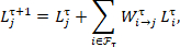
Subsequently, the secondary failure-state update is verified via a binary survival function :

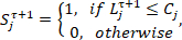
A node is declared failed () when its transient load exceeds its capacity, updating the failure set F_τ+1. The cascade reaches steady state when F_τ+n = ∅, indicating that no additional nodes have failed in the current micro-time step and all surviving nodes operate within their capacity boundaries.

The cascading loop continues until no additional nodes fail, marking the arrival at a secondary steady state where the cascade potential is fully dissipated.

System resilience evaluation and threshold identification

The fourth stage evaluates system resilience by monitoring the macro-disintegration rate of the digital ecosystem graph. The relative scale of the largest connected component derived from surviving nodes is continuously extracted to plot the phase transition decay curve over the fraction of removed nodes. The global transmission efficiency E(τ) is calculated to quantify the connectivity of the surviving topology

where N is the initial total number of nodes (a constant), A_τ is the set of surviving active nodes, and is the directed shortest geodesic distance from node i to j at the current step. The critical transition threshold is then identified by monitoring the mutation of the first derivative of this efficiency function with respect to the removal ratio. This threshold is determined as the point at which the first derivative attains its minimum value, indicating the steepest decline in transmission efficiency. The critical resilience threshold is calculated by numerically differentiating the global transmission efficiency E(τ) with respect to the node removal ratio f using a second-order central difference scheme. The first derivative trajectory dE/df is smoothed with a moving average window of five consecutive data points to reduce Monte Carlo sampling noise while preserving the location of the steepest descent. The critical threshold fc is selected as the removal ratio at which the smoothed first derivative attains its global minimum value, corresponding to the point of maximum decay rate in transmission efficiency. This selection criterion is applied consistently across all simulation scenarios and baseline models. The reported threshold value of 12.41% ± 0.63% represents the mean and standard deviation computed from 100 independent Monte Carlo simulations with different random seeds, ensuring statistical robustness of the phase transition localization.

Simulation configurations and baseline implementations

To ensure fully reproducible simulations, random seeds were sequentially assigned (integers 1 through 100) prior to each Monte Carlo iteration. The topological evolution and statistical modeling were executed using R with the tergm package, while the nonlinear cascading simulations were implemented in Python using the NetworkX library. Furthermore, for the comparative deep learning baseline, the GCN-Attack model was implemented using PyTorch Geometric. It was constructed with a standard two-layer Graph Convolutional Network architecture (hidden dimension of 64), and trained using the Adam optimizer with a learning rate of 0.01 for 200 epochs to ensure rigorous and consistent experimental control across baseline evaluations.

Résultats

The overall execution logic and data flow of the proposed physical computation framework are illustrated in Figure 1. As the framework executes, the microscopic thermal characteristics of local overflow load redistribution and the nonlinear evolution of node degree distributions are captured (overviewed in Figure 2 and Figure 3, with dynamic details described below. The subsequent sections map the simulation outcomes directly to the protocol stages.

Temporal topology evolution via TERGM

Figure 4 visually deconstructs the spatial topology and community structure of the ICT-DE500 core network, highlighting the distribution of high-betweenness nodes targeted in deliberate attack simulations. The goodness-of-fit test confirms that the generated network topology effectively models the temporal evolution of real ecosystems, successfully avoiding gradient explosion or traps of local optimality after the 10,000-step burn-in period. Figure 5 presents the MCMC-MLE parameter convergence diagnostic trajectories and the geodesic distance goodness-of-fit. Figure 5A shows that the three core parameters representing edge density θ₁, mutuality θ₂, and geometrically weighted edgewise shared partnership θ₃ all terminate their large directional drift after crossing the 10,000-step burn-in threshold, with expected means converging and stabilizing near the horizontal baseline. Figure 5B demonstrates that the empirical observations of shortest geodesic distances fall robustly within the overall distribution boundaries of 1,000 independent network realizations. These realizations were extracted using a thinning interval of 10 from the 10,000 sequential Gibbs sampling iterations to minimize autocorrelation, confirming the reliability of the topology generation base. The specific MCMC-MLE parameter estimates, standard errors, and statistical significance for endogenous structural effects across the observation years are detailed in Table 2.

The temporal evolution of macroscopic topological structure is quantified in Figure 6. The network density steadily increased from 0.015 to 0.035 between 2018 and 2023, while the average clustering coefficient rose from 0.22 to 0.37, highlighting a significant density-cluster divergence phenomenon. The density rises most sharply between 2020 and 2021, fluctuating from 0.021 to 0.029, whereas the clustering coefficient reaches a local peak of approximately 0.31 in 2020 and subsequently drops to approximately 0.29 despite rapid density growth in 2021. This divergence reveals the adaptive evolution mechanism under macroeconomic cycle fluctuations, where risk-avoidance grouping in 2020 drives local clustering, while massive new cross-border connections in 2021 temporarily dilute the close-knit community structure.

Physical capacity calibration and load initialization

The bivariate sensitivity analysis in Figure 7 examines the joint effect of physical capacity redundancy and load polarization on the phase transition trajectory of the largest connected component. Across the nine orthogonal combinations of capacity tolerance α and load heterogeneity β, the array of panels shows that increasing α and decreasing β both delay network collapse. Under the polarized load scenario with β = 1.5 and minimal redundancy α = 0.1 in Figure 7A, the critical collapse threshold is approximately f_c = 0.08. Raising α to 0.5 in Figure 7C shifts the inflection point rightward to f_c ≈ 0.23. Under the balanced load scenario with β = 1.0 and α = 0.1 in Figure 7G, the threshold remains robust at f_c ≈ 0.18, and at the optimal combination α = 0.5 and β = 1.0 in Figure 7I, the threshold extends significantly to f_c ≈ 0.38. These results demonstrate that load balancing produces a greater marginal gain in resilience than capacity expansion alone.

Nonlinear cascading dynamics under deliberate attacks

As introduced in the framework overview, the microscopic thermal characteristics of local overflow load redistribution following the initial cascade failure are shown in Figure 2, and the nonlinear evolution of node degree distribution across three typical micro-time steps is presented in Figure 3.

System resilience evaluation and threshold identification

The critical transition threshold for global transmission efficiency is located at 12.41% ± 0.63% node removal during a targeted attack. In the context of the 500-node network, this proportion corresponds to the targeted removal of approximately 62 core hub nodes. This threshold marks the efficiency-collapse point (i.e., the onset of the steepest decline in transmission efficiency) rather than a complete topological disconnection. Figure 8 presents the three-dimensional evolution surface of global efficiency E(τ) over removal ratio and peak network load in Figure 8A, and the two-dimensional cross-section with numerical differentiation in Figure 8B. When the removal ratio f is below 0.10, E(τ) remains above 0.8 and the first derivative oscillates in a shallow region. The minimum of the first derivative trajectory identifies the critical transition threshold, with Figure 8B displaying a single-run cross-section at f_c = 12.0% that is highly consistent with the statistical mean from 100 independent Monte Carlo simulations.

Simulation configurations and baseline implementations

The proposed model significantly outperforms the static and deep learning baselines under targeted attack scenarios. However, under random failure conditions, the Static BA-ML baseline exhibits a higher survival threshold (49.12%) compared to the TERGM-ML model (46.28%). It is important to note that the comparison with the Static BA-ML model serves as a distinct topological benchmark rather than a strictly controlled ablation, as the Barabási-Albert generative mechanism fundamentally differs from the ERGM framework. Figure 9 displays the raincloud plot of cascade propagation peak velocities across four model architectures. The Static BA-ML baseline shows a median peak velocity of approximately 49.7 nodes per step, with extreme batches approaching 140. The SNA-Cascading and GCN-Attack models have medians of approximately 35.6 and 23.9, respectively. The TERGM-ML model exhibits the strongest convergence with a median of 13.2 nodes per step, almost eliminating extreme collapses exceeding 40. Table 3 summarizes the critical thresholds and statistical significance for all models. These comparisons clarify that while the TERGM-ML framework demonstrates superior structural resilience to targeted asymmetric shocks, the observed performance differences reflect the joint influence of distinct underlying topologies, temporal evolution, and capacity-aware redistribution, rather than being solely attributable to isolated mechanism ablations.

DATA AVAILABILITY:

The raw data used in this study are derived from the Crunchbase global corporate investment and merger database, publicly accessible via the Kaggle platform at https://www.kaggle.com/datasets/justinas/startup-investments. The processed ICT-DE500 subset, consisting of 500 entities with annual edge matrices for the period 2018–2023 and node attribute data including degree and betweenness centrality, along with the TERGM estimation and convergence diagnostic scripts, the cascading failure simulation code with the improved Motter-Lai algorithm, and the complete dependency specifications, have been deposited in a publicly accessible GitHub repository at https://github.com/moonmoon1189/digital-economy-resilience-complex-networks.

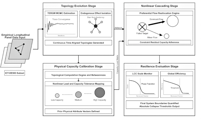
Figure 1: Temporal topology evolution and nonlinear cascade physical computation framework. This figure illustrates the overall execution logic and data flow, including topology evolution, physical capacity calibration, nonlinear cascading, and resilience evaluation stages for identifying the critical transition threshold. Please click here to view a larger version of this figure.

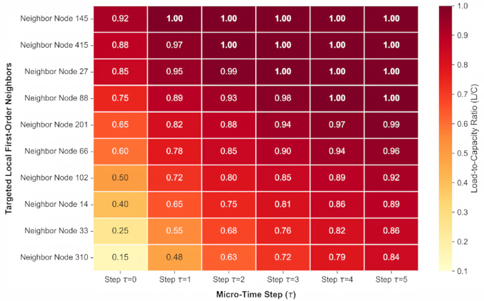
Figure 2: Thermal diagram of the microscopic evolution of nonlinear load redistribution and local cascade overload. The figure illustrates the dynamic thermal characteristics of the local redistribution of overflow load after the initial cascade failure from micro-time step 0 to step 5. Please click here to view a larger version of this figure.

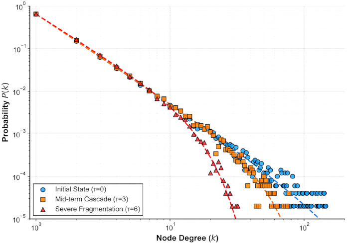
Figure 3: Scatter plot of nonlinear evolution of node degree distribution during cascading failure. The figure presents the evolution trajectory of the node degree distribution of the system at three typical micro-time steps (0, 3, 6). Please click here to view a larger version of this figure.

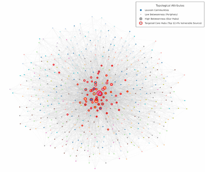
Figure 4: Spatial topology, community structure, and deliberate attack target distribution of the ICT-DE500 core network. The figure visually deconstructs the highly nonlinear macroscopic topology and microscopic node attributes of the core network, highlighting star hubs and vulnerable sources. Please click here to view a larger version of this figure.

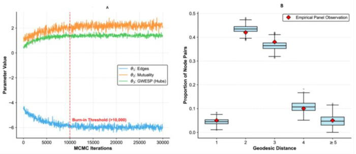
Figure 5: Goodness-of-fit test of Markov Chain Monte Carlo parameter diagnostic trajectory and geodesic distance. (A) This panel shows the diagnostic trajectory of MCMC-MLE parameter estimation across iterations, while panel (B) displays the goodness-of-fit test of the shortest geodesic distance. Please click here to view a larger version of this figure.

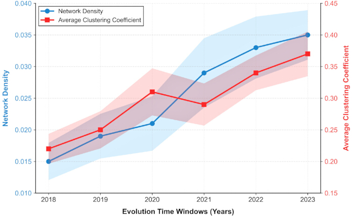
Figure 6: Joint distribution of macro-topological feature parameters in time series evolution. The figure shows the changing trend of macro-topological parameters, specifically network density and average clustering coefficient, for the digital economy ecosystem between 2018 and 2023. The shaded regions around the trend lines represent the 95% confidence intervals derived from 100 independent Monte Carlo simulations. Please click here to view a larger version of this figure.

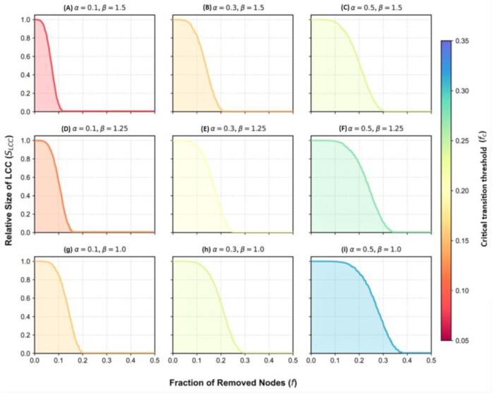
Figure 7: Array plot of phase transition decay for bivariate sensitivity to capacity tolerance and load heterogeneity. (A–I) These panels display the phase transition trajectories across various orthogonal combinations of capacity tolerance and load heterogeneity. Please click here to view a larger version of this figure.

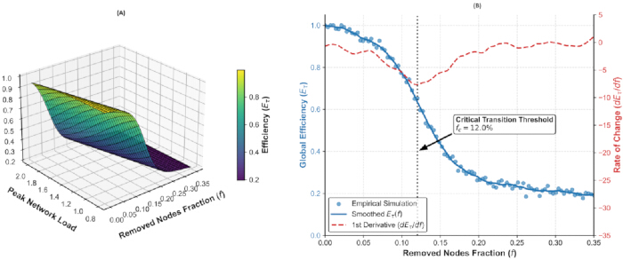
Figure 8: Joint profile of global transmission efficiency in three dimensions and cross-sectional critical transition threshold. Panel (A) constructs the three-dimensional spatial evolution of global transmission efficiency, and panel (B) extracts the two-dimensional cross-sectional critical transition threshold (i.e., the efficiency-collapse point) localization using numerical differentiation. Please click here to view a larger version of this figure.

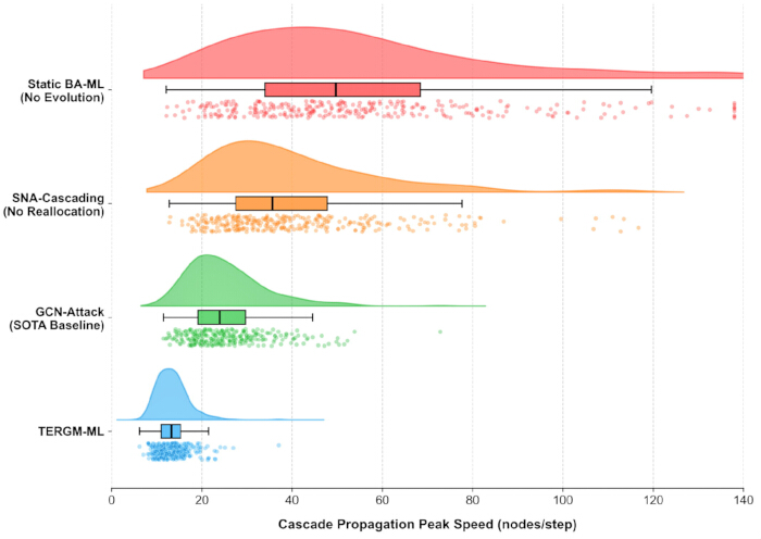
Figure 9: Heterogeneous distribution of cascade propagation peak evolution velocity in raincloud plot. The figure comprehensively displays the heterogeneous probability density distribution of the cascade propagation peak velocities of four models during secondary disaster outbreaks. Please click here to view a larger version of this figure.

Parameter	Variable & Range	Constraint & Justification
Network Scale	N=500	Fixed size of the extracted ICT-DE500 empirical network subset.
Centrality Weight	λ=0.5	Anchored baseline ensuring equal weighting for degree and betweenness.
Load Allocation Index	β∈[1.0,1.5]	Non-linear exponent controlling initial business load heterogeneity.
Capacity Tolerance	α∈[1.0,1.5]	System-level redundancy ratio defining the upper bound of physical capacity.
MCMC Burn-in Period	>10,000 steps	Mandatory initial iterations discarded to achieve stationary distribution.
Gibbs Sampling Iterations	>10,000 steps	Sequential sampling steps to generate time-aligned network topologies.

Table 1: Core parameter settings for time-series evolution and cascading failure physical simulations. The table defines the core parameters, including network scale, centrality weight, load allocation index, capacity tolerance, and Markov Chain Monte Carlo (MCMC) iterations.

Observation Year	Edge Density (θ1) Estimate	Edge Density (θ1) Std.Error	Mutuality (θ2) Estimate	Mutuality (θ2) Std.Error	GWESP (θ3) Estimate	GWESP (θ3) Std.Error	Significance
2018	-6.35	0.12	1.95	0.08	1.25	0.05	***
2019	-6.15	0.11	1.98	0.09	1.35	0.06	***
2020	-6.05	0.14	2.15	0.1	1.55	0.07	***
2021	-5.85	0.13	1.9	0.09	1.3	0.06	***
2022	-5.75	0.12	2.05	0.08	1.42	0.05	***
2023	-5.65	0.11	2.1	0.07	1.48	0.05	***

Table 2: TERGM parameter estimates for endogenous structural effects across observation years (2018–2023). The table reports the Markov Chain Monte Carlo Maximum Likelihood Estimation (MCMC-MLE) parameter estimates, standard errors, and statistical significance for edge density, mutuality, and geometrically weighted edgewise shared partnership across the six annual observation periods. ***p < 0.001. Standard errors are reported next to parameter estimates.

Model Architecture	Temporal Evolution Mechanism	Dynamic Reallocation Mechanism	Critical Threshold (Targeted Attack)	Critical Threshold (Random Failure)	Statistical Significance (p-value)
TERGM-ML	Yes	Yes	12.41% ± 0.63%	46.28% ± 1.75%	Reference Baseline
Static BA-ML	No	Yes	7.85% ± 0.42%	49.12% ± 1.88%	p < 0.001 ***
SNA-Cascading	Yes	No	8.93% ± 0.55%	37.54% ± 1.42%	p = 0.003 **
GCN-Attack (SOTA Baseline)	Implicit	Implicit	10.76% ± 0.81%	43.15% ± 2.05%	p = 0.021 *

Table 3: Comparison of core mechanism ablation and multimodel architecture resilience boundary. The table details the critical thresholds and statistical test results for system resilience of time-series graphs and improved Motter-Lai (TERGM-ML) and three baseline models under both deliberate attack and random failure scenarios. Values are reported as mean ± standard deviation based on 100 independent Monte Carlo simulations. Targeted attack refers to the sequential removal of nodes based on descending betweenness centrality. Statistical significance evaluates the difference in the Targeted attack threshold between the respective baseline model and the proposed framework using an independent two-sample t-test (*p < 0.05, **p < 0.01, ***p < 0.001).

Discussion

Le cadre de calcul physique en cascade proposé, combinant des graphes temporels à joints et un modèle Motter-Lai amélioré (TERGM-ML), atténue efficacement les limites de type boîte noire des modèles purement basés sur les données dans la prédiction de la résilience. Ce cadre s'appuie sur les modèles graphiques exponentiels fondamentaux introduits par Wasserman et Pattison¹¹ et sur le cadre d'attaque basé sur les cascades initialement développé par Motter et Lai¹², tout en étendant ces deux approches afin de prendre en compte la dynamique temporelle et les contraintes locales de capacité. Ce paradigme associe étroitement l'évolution topologique endogène réelle aux limites de charge des micro-entités en introduisant une logique de flux sélectif fondée sur des contraintes locales liées aux seuils physiques de capacité. Le mécanisme d'évolution temporelle suit les spécifications du TERGM pour la modélisation dynamique des réseaux^13,14, tandis que la stratégie d'allocation des capacités s'aligne sur les principes de conception redondante des réseaux visant à atténuer les défaillances en cascade^15,16.

Une étape cruciale du protocole réside dans le mécanisme optimal de reroutage du flux opérationnel sous-jacent en fonction de la capacité disponible des voisins, remplaçant l'hypothèse irréaliste d'une « répartition moyenne » utilisée dans le modèle traditionnel de Motter-Lai. L'hypothèse de redistribution uniforme du modèle standard de Motter-Lai a été critiquée dans des études récentes sur la résilience des infrastructures pour avoir négligé les contraintes hétérogènes de capacité des nœuds^6,10. Les résultats actuels indiquent que le réseau communautaire en boucle fermée sous-jacent exerce un effet d'amortissement physique défini sur les pics de charge en surcharge, supprimant efficacement la propagation en cascade et retardant de manière significative la désintégration par transition de phase de l'efficacité globale de transmission. Le modèle TERGM-ML présente le seuil critique le plus élevé face aux attaques ciblées, atteignant 12,41 % ± 0,63 %, ce qui reflète la capacité d'amortissement de l'architecture endogène du réseau et atténue le risque d'avalanche globale induit par un point unique de surcharge. L'augmentation du seuil critique, passant de 7,85 % à 12,41 %, provient de deux mécanismes synergiques. Le mécanisme d'évolution temporelle génère des structures communautaires en boucle fermée et des liens réciproques absents dans les réseaux sans échelle statiques. Ces communautés limitent spatialement la propagation de la surcharge en forçant la charge excédentaire à emprunter plusieurs chemins intra-communautaires avant d'atteindre des régions éloignées, chaque étape de traversée dissipant une fraction de la charge transitoire par absorption via les nœuds voisins. Le mécanisme de redistribution dynamique dirige la charge en surcharge exclusivement vers les voisins disposant d'une capacité résiduelle positive ΔC_j(τ) > 0, évitant ainsi la répartition uniforme qui épuise rapidement la redondance locale dans le modèle standard de Motter-Lai. Les communautés en boucle fermée fournissent la structure topologique qui rend le routage sensible à la capacité efficace, tandis que le routage sensible à la capacité empêche la saturation prématurée des liens internes à la communauté. Ce couplage explique pourquoi le cadre combiné surpasse de plus de 4 points de pourcentage le modèle statique de référence en termes de seuil critique. Cette valeur seuil est conforme aux prédictions théoriques pour les réseaux sans échelle soumis à des attaques ciblées¹⁷ et aux comportements de transition de phase de percolation observés dans les systèmes complexes¹⁸.

Malgré ces avancées, la méthode présente certaines limitations. Limitées par les frontières observationnelles existantes, les extrapolations actuelles reposent fortement sur des tranches centralisées et complètes de la topologie globale, et leurs fenêtres temporelles d'échantillonnage discrétisées ne peuvent pas capturer précisément les perturbations d'impédance variant à micro-échelle de temps causées par des oscillations environnementales externes soudaines à haute fréquence. Ces limitations reflètent les défis identifiés dans des revues récentes portant sur les métriques de résilience pour les systèmes cyber-physiques et la modélisation des défaillances en cascade dans des conditions dynamiques^19,20. Les recherches et applications futures pourraient s'orienter vers des architectures décentralisées, en se concentrant sur l'exploration de mécanismes dynamiques de compensation adaptative de la résilience fondés sur une collaboration distribuée multi-agents dans des conditions de jeux à information incomplète. L'abstraction par graphe monocouche et l'attribution globale des paramètres constituent des limitations majeures du cadre actuel. Des études sur les réseaux multicouches ont montré que les interdépendances entre couches d'interaction peuvent amplifier ou atténuer la propagation en cascade d'une manière que les modèles monocouches ne peuvent pas rendre. L'attribution globale de la tolérance de capacité α et de l'exposant d'allocation de charge β fait abstraction de l'hétérogénéité spécifique aux entités en matière de marges de capacité et de sensibilité à la charge. Trois extensions méritent d'être explorées dans des travaux futurs : remplacer la topologie monocouche par une représentation multicouche distinguant les flux de capitaux, les licences technologiques et la prestation de services comme couches distinctes avec des dépendances inter-couches ; calibrer les paramètres spécifiques aux entités concernant la capacité et la charge à partir de données opérationnelles au niveau des entreprises ; et passer des tranches centralisées de topologie à des architectures multi-agents décentralisées, dans lesquelles les nœuds prennent des décisions adaptatives de redistribution basées sur des signaux localement observables. Des études récentes sur les réseaux multicouches ont démontré que les interdépendances entre couches d'interaction distinctes peuvent amplifier ou atténuer la propagation en cascade d'une manière que les modèles monocouches ne peuvent pas capturer.

Matériaux

Liste des matériaux utilisés dans cet article

Nom	Entreprise	Numéro de catalogue	Commentaires
AMD EPYC 7742 CPU	Advanced Micro Devices	7742	Processeur haute performance pour l'exploration des structures de graphes et le recalcul des plus courts chemins.
Base de données Crunchbase	Kaggle	investissements de démarrage	Investissement mondial des entreprises et M&Un réseau enregistré utilisé comme base de réseau global.
CUDA 11.6	NVIDIA	version 11.6	Plateforme d'accélération matérielle utilisée pour les opérations tensorielles dans le modèle de base GCN.
NetworkX 2.8	Développeurs de NetworkX	version 2.8	Bibliothèque d'analyse de réseaux complexes utilisée pour l'extraction de paramètres de graphes et la recherche de chemins.
NumPy	Développeurs de NumPy	N/A	Cadre de noyau mathématique garantissant une logique déterministe et éliminant la dérive numérique.
NVIDIA RTX 3090 GPU	NVIDIA	RTX 3090	Processeur graphique utilisé pour accélérer les calculs tensoriels dans la base de référence de l'apprentissage profond.
Python 3.9	Fondation Python	version 3.9	Environnement d'exécution sous-jacent pour le cadre principal compilé et exécuté.
PyTorch 1.12	Meta IA	version 1.12	Bibliothèque d'apprentissage profond utilisée pour les graphes de calcul et la propagation avant dans le modèle de référence.
R	/	version 4.2.2	/
package statnet	Le projet statnet	N/A	Package statistique avancé d'expansion utilisé pour la méthode TERGM à réseaux dynamiques multi-étapes MCMC-MLE.
paquetage tergm	/	version 4.2.0	/
Ubuntu 22.04.1 LTS	Canonique	22.04.1 LTS	Configuration du système d'exploitation du serveur hébergeant la matrice computationnelle multithread.