本プロトコルでは、相補的なEEG表現、デュアルスペース視覚アライメント、および拡散デコードを組み合わせたEEG-画像再構成フレームワークであるTri-stream Disentangled Network (TDE-Net)について提示します。
方法論記事
THINGS-EEG2における脳波ベースの画像再構成に向けた、適応的デュアルスペース融合を備えた3ストリームもつれ解消ネットワーク
この記事について
サマリー
要約
Reconstructing visual stimuli from non-invasive electroencephalography (EEG) requires mapping short, noisy neural responses to meaningful visual representations despite limited spatial sampling. Existing EEG-to-image approaches employ diverse neural representations and generative strategies, necessitating reproducible workflows that disentangle structural and semantic contributions. This protocol presents the Tri-stream Disentangled Network (TDE-Net), a computational framework for EEG-based image reconstruction. The protocol uses preprocessed THINGS-EEG2 recordings and organizes EEG information into a raw EEG anchor, a sample-specific functional graph stream, and a multi-scale temporal semantic stream. The graph stream captures frequency-domain relationships among EEG channels via graph convolution and cross-trial contrastive learning, while the semantic stream extracts task-relevant features via adaptive spatial weighting and multi-scale temporal convolutions. Structural and semantic features are mapped separately to variational autoencoder (VAE) and Contrastive Language-Image Pre-training (CLIP) latent spaces, combined using development-set-selected fusion weights, and decoded using Stable UnCLIP. Across 10 participants, TDE-Net achieved a mean CLIP pairwise identification accuracy of 0.8135, with complementary metrics demonstrating structural and feature-space correspondence. Ablation and representation-level analyses further characterized the contributions of individual streams. This protocol provides a reproducible framework for investigating complementary EEG representations and diffusion-based visual reconstruction.
概要
視覚知覚のデコーディングは、ブレイン・コンピューター・インターフェース(BCI)および認知神経科学における学際的な研究領域です。機能的磁気共鳴画像法(fMRI)によって現実的な画像の再構成が可能になりましたが1,2,3,4、そのコスト、限定的な携帯性、および血流動態による遅延が、一部のアプリケーションにおいて制限となっています。脳波測定(EEG)は、比較的導入しやすい装置でミリ秒単位の時間分解能での測定が可能ですが、信号対雑音比(SN比)が低く、空間的なサンプリングが限定的であるため、EEGから画像への再構成は困難です。
手法の複雑さは、一般的なバイアス・バリアンスのトレードオフ5の観点から解釈されるべきである。初期の視覚デコーディング手法では浅い表現や線形表現が用いられていたが、その後の研究では、コンパクトな畳み込み、グラフベース、およびアテンションベースのエンコーダが導入された6,7,8,9,10,11。クロスモーダルアライメントも、マルチモーダル特徴量学習12,13から、潜在拡散モデルや大規模視覚エンコーダ14,15,16へと発展してきた。これらのアプローチは有用なベースラインを確立しているが、入力表現、潜在ターゲット、およびデコーダが異なるため、結果はそれぞれの実験設定の中で解釈されるべきである。
TDE-Netの目的は、構造的および意味的なEEG表現を分離し、それらを相補的な視覚潜在空間にアライメントさせ、これらの予測を統合して拡散ベースの画像再構成を行うモジュール式EEG-画像再構成フレームワークを提供することです。近年のEEG-視覚デコーディング研究では、EEG-CLIPにおけるTransformerベースのEEG誘導生成17、FSDBNにおけるダイナミック脳ネットワークを用いた前景認識アライメント18、情報制約付きアライメントによる認知誘導適応ブラーリング19、およびマルチレベル双方向バイオミメティック学習20などが導入されています。PerceptogramやEEG埋め込みに基づく誘導拡散を含む関連するEEG-画像パイプラインは、潜在予測のためのさらなる参照を提供しています21,22。TDE-Netはモデル構成において異なります。本モデルは、生のEEGアンカー、サンプル固有の機能的グラフ表現、および時間的な意味表現を明示的に分離し、融合前にVAE空間およびCLIP空間への非対称アライメントを行います。この構成により、潜在空間および画像レベルの解析を通じて、構造的および意味的な寄与を個別に検討することが可能になります。単一の表現を用いる手法や直接的にアライメントさせるEEG-画像アプローチと比較して、このモジュール設計は構造的および意味的な経路を個別に提供し、潜在予測中に線形なEEGリファレンスを保持し、アブレーション解析および潜在空間解析を通じて各表現の寄与を独立して評価することを可能にします。
TDE-Netは、ペアリングされたEEG応答と視覚刺激があり、十分なトレーニング条件が整い、かつ意味的再構成を主目的とする短い刺激後ウィンドウを用いた実験向けに設計されています。その段階的な構成により、特徴抽出、潜在空間のアライメント、融合、および拡散デコーディングを個別に検証することが可能です。線形マッピングは、非常に小規模なデータセットや、モデルの複雑さを最小限に抑えることを優先する設定に適していますが、タスク固有の大規模なデータセットがあり、リアルタイムでの展開が可能な場合は、エンドツーエンドのニューラルデコーダーが好ましいと考えられます。
本プロトコルでは、THINGS-EEG2の高速逐次視覚提示(RSVP)設定における提案構成を評価します。主な貢献としては、生の線形アンカー、サンプル固有の機能グラフストリーム、およびマルチスケール時間的意味ストリームからなる3ストリームのEEG表現スキームが挙げられます。これらの相補的な表現はVAEおよびCLIPの潜在空間にマッピングされ、対応する予測は拡散デコーディングの前に統合されます。本フレームワークは、被験者レベルの再構成指標、アブレーション解析および時間窓解析、そして表現レベルの可視化を用いて、THINGS-EEG2の全10被験者で評価され、空間アテンションマップは頭皮チャネル(トポグラフィック)解析として解釈されます。
プロトコル
The protocol comprises six sequential stages: preparation of EEG trials and image latents; construction of the graph structural stream; training of the semantic EEG encoder; fitting of the CLIP/VAE mappings; fusion of the latent predictions, followed by image decoding; and evaluation of image-level and representation-level outcomes (Figure 1).
1. Prepare EEG trials and image embeddings
- Document the source cohort and acquisition protocol.
NOTE: The source cohort comprised 10 healthy adults (mean age 28.5 years, SD 4.0; eight female and two male) with normal or corrected-to-normal vision. Participants provided written informed consent, received monetary compensation, and completed the original protocol with approval from the ethics committee of the Department of Education and Psychology at Freie Universität Berlin, in accordance with the Declaration of Helsinki23.- Use the publicly available THINGS-EEG2 dataset as a secondary-analysis resource.
- Use the source partition of 1,654 training concepts and 200 non-overlapping test concepts drawn from THINGS, with the proportions of 27 higher-level categories balanced between partitions. Select ten natural-background images for each training concept and one image for each test concept, to yield 16,540 training conditions and 200 held-out test conditions.
NOTE: In the present study, the target-detection task used separate Buzz Lightyear catch images that were excluded from the present reconstruction analysis23. - Follow the timing of the original rapid serial visual presentation protocol when interpreting the epochs.
NOTE: Each sequence began with a 750 ms blank interval, followed by 20 centrally presented images. Each image subtended 7 degrees of visual angle, remained on screen for 100 ms, and had a 200 ms stimulus-onset asynchrony, corresponding to 5 images/s. A second 750 ms blank interval preceded a response period of up to 2 s, during which participants first blinked and then reported whether a target image had appeared. A central bull's-eye fixation target remained visible throughout the sequence23. - Account for the original recording-session structure when organizing the dataset. Use data from the four recording sessions completed by each participant, with each session comprising four test runs and 15 training runs of approximately 5 min each. Retain four repetitions for each training condition and 80 repetitions for each test condition, corresponding to 82,160 analyzed non-target image trials per participant23.
- Use the EEG data acquired with the original THINGS-EEG2 recording configuration. These recordings were acquired at 1,000 Hz using a 64-electrode EASYCAP arranged according to the international 10-10 system and a BrainVision actiCHamp amplifier, with Fz as the online reference and an online 0.1–100 Hz band-pass filter.
- Use the released preprocessed data, which were epoched from -200 to 800 ms relative to image onset, baseline-corrected using the prestimulus interval, downsampled to 100 Hz, restricted to 17 parieto-occipital channels, cleared of target trials, and subjected to multivariate noise normalization independently within each recording session23.
- Prepare EEG trial tensors
- Load the released preprocessed THINGS-EEG2 tensors for all 10 participants. From each source epoch, select the 0–800 ms post-stimulus interval and the 17 parieto-occipital channels, retaining the 100 Hz sampling rate to obtain 80 time points per trial. Preserve the source partition of 16,540 training image conditions and 200 held-out test image conditions for each participant23 (Figure 2).
- For graph-stream pre-training, retain the four independent training repetitions for each image condition and sample two repetitions to form a positive pair. For the raw and semantic streams, average the four training repetitions and average the 80 available test repetitions for each condition.
- Use the preprocessed THINGS-EEG2 tensors produced by the original MVNN pipeline; within each implemented feature extractor, apply the documented file-level Z-scoring before feature computation.
NOTE: This asymmetric use of repetitions is deliberate: repeated trials provide positive pairs for graph-stream contrastive pre-training, whereas the raw and semantic streams use condition-level averages for supervised mapping. The resulting design combines repetition-level invariance learning in the structural stream with condition-level latent prediction in the raw and semantic streams.
- Prepare paired image latents
- Use the 1,024-dimensional CLIP vision encoder and the VAE encoder associated with sd2-community/stable-diffusion-2-1-unclip to extract paired image targets. Resize VAE input images to 768 x 768 pixels, store the VAE posterior mode as a 36,864-dimensional vector (4 x 96 x 96), and preserve the image-condition order.
- Save three input forms: repeated-trial tensors for graph contrastive learning, averaged EEG tensors for the raw and semantic streams, and paired CLIP/VAE image latents for supervised mapping.
- Normalize and cache the inputs
- Cache the preprocessed EEG tensors, extracted graph and semantic features, and paired image latents with fixed condition ordering.
- During ridge mapping, estimate feature-wise standardization parameters from the training inputs and apply those parameters to the development and test inputs.
2. Construct the graph structural stream
- Construct the graph stream from repeated training trials and export node-level features after contrastive pre-training. Use the same graph construction rule for test feature extraction, without using test image latents during feature computation.
- Transform EEG trials into frequency-domain graph inputs
- Transform each trial with an 80-point fast Fourier transform (FFT) and retain the first 40 nonnegative-frequency bins, spanning 0 Hz–48.75 Hz at the 100 Hz sampling rate. Use the log-amplitude spectrum as a 17 x 40 node-feature matrix X. For each EEG sample, calculate C_ij = |corr(X_i, X_j)| between every pair of the 17 channel feature vectors.
- In each row, retain the diagonal self-correlation and the three strongest off-diagonal correlations (k = 4 retained entries including self), then symmetrize the retained matrix to define the sample-specific weighted functional adjacency A. Apply symmetric degree normalization before graph convolution.
- Use this construction during training and testing; electrode physical coordinates are not used to define a fixed graph.
NOTE: Retaining self-connectivity preserves each node's signal, whereas limiting cross-channel connections to 3 per row controls graph density prior to symmetrization. The frequency-domain representation provides a compact amplitude-based description for graph construction, but does not preserve phase or all fine-grained phase-locked ERP timing; those temporal aspects remain available in the raw anchor and semantic temporal streams.
- Aggregate electrode topology with spectral graph convolution
- Apply a five-layer graph convolutional network (GCN)24 with 80 hidden units per layer, ReLU activations, 0.3 dropout, symmetric degree normalization, and mean graph pooling.
- Use an 80-dimensional two-layer projection head for the contrastive objective, and export the 17 x 80 node-level representation for structural fusion. Apply spectral graph convolution to the input-dependent adjacency matrix; do not introduce a separate dynamic convolution operator.
- Train the graph stream with cross-trial contrastive learning
- Within the training partition, randomly select two repetitions from the same image condition as a positive pair and treat representations from other conditions in the batch as negatives. Optimize the InfoNCE contrastive objective25 with temperature τ = 0.5, batch size 32, Adam with learning rate 5 x 10⁻⁴, 20 epochs, cosine annealing to eta_min = 10–6, and random seed 42.
 (1)
(1) - Define cosine similarity in the contrastive objective and use the indicator function to identify paired repetitions. Keep the projection dimension at 80 and apply the same temperature to both directions of the contrastive loss.
- Within the training partition, randomly select two repetitions from the same image condition as a positive pair and treat representations from other conditions in the batch as negatives. Optimize the InfoNCE contrastive objective25 with temperature τ = 0.5, batch size 32, Adam with learning rate 5 x 10⁻⁴, 20 epochs, cosine annealing to eta_min = 10–6, and random seed 42.
- Export node-level graph features for early fusion
- Freeze the graph encoder after pre-training and export the 17-channel node features with 80 dimensions per node. Concatenate these features with the averaged raw EEG along the feature dimension to obtain the raw-plus-graph structural input for VAE mapping.
- Save the resulting raw-plus-graph feature tensor and use it only as the structural input to the VAE regression branch.
3. Train the semantic EEG encoder
- Train the semantic EEG encoder on the averaged 17-channel, 80-point EEG tensors.
- Optimize cosine embedding loss with AdamW (learning rate 5 x 10⁻⁴; weight decay 0.01), batch size 64, 50 epochs, cosine annealing to eta_min = 10–6, random seed 42, and a 1,024-dimensional output.
- Apply data-driven adaptive spatial filtering
- Apply a learnable tensor-product channel weighting operation to the input EEG tensor and expand the representation to a depth of 9. Treat this operation as a data-driven channel-weighting layer rather than an implementation of the classical Common Spatial Pattern (CSP) spatial filter26.
 (2)
(2) - Use the learned channel-weighting operation to produce nine feature maps, then pass them to the multi-scale temporal convolution block.
- Apply a learnable tensor-product channel weighting operation to the input EEG tensor and expand the representation to a depth of 9. Treat this operation as a data-driven channel-weighting layer rather than an implementation of the classical Common Spatial Pattern (CSP) spatial filter26.
- Model temporal receptive fields at multiple scales
- Apply three parallel temporal convolutions with kernel sizes 5, 15, and 31 samples, using same-length padding. Concatenate the three outputs to obtain 24 temporal feature channels and apply batch normalization and GELU activation.
 (3)
(3)
NOTE: The convolutions provide multi-scale temporal receptive fields within the broader temporal convolutional modeling framework27. - Use the three kernel sizes as multi-scale temporal filters; interpret their output as learned signal representations rather than as direct assignments to specific ERP components.
- Apply three parallel temporal convolutions with kernel sizes 5, 15, and 31 samples, using same-length padding. Concatenate the three outputs to obtain 24 temporal feature channels and apply batch normalization and GELU activation.
- Recalibrate task-relevant feature channels
- Apply depth attention with adaptive average pooling to the temporal dimension and a kernel-7 convolution followed by Softmax normalization, consistent with channel-recalibration principles28. Multiply the resulting attention weights element-wise with the multi-scale feature tensor.
 (4)
(4) - Use the attention output as the input to the spatial convolution block and do not interpret the learned weights as causal neural localization.
- Apply depth attention with adaptive average pooling to the temporal dimension and a kernel-7 convolution followed by Softmax normalization, consistent with channel-recalibration principles28. Multiply the resulting attention weights element-wise with the multi-scale feature tensor.
- Export the global semantic EEG feature
- Apply a 1 x 1 convolution followed by a depthwise convolution spanning the 17 electrode channels, batch normalization, GELU activation, average pooling with factor 2, and dropout p = 0.5. Flatten the result and project it to a 1,024-dimensional semantic feature vector.
- Save one 1,024-dimensional semantic feature vector for each averaged EEG sample.
4. Map EEG features to CLIP and VAE latent spaces
- Pair each EEG feature tensor with the image latent having the same condition index. Fit separate mappings for CLIP and VAE targets, and keep all image conditions in the training partition disjoint from those in the held-out test partition.
- Fit ridge regression29 with an intercept and a maximum of 50,000 iterations. Use λCLIP = 1,000 for the raw-to-CLIP and semantic-to-CLIP mappings, λVAE = 0 for the raw-to-VAE anchor, and λVAE, struct = 1,000 for the structural-stream-to-VAE mapping. Standardize mapping inputs using fit-partition statistics.
NOTE: The structural stream is the concatenation of raw EEG and graph features; the semantic stream contains the semantic encoder output without raw-feature concatenation. - Map structural features to the VAE latent space
- Fit the structural-stream-to-VAE ridge mapping with λVAE,struct = 1,000 and predict the 36,864-dimensional VAE latent. This branch receives the concatenated raw EEG and graph representations; it is the only nonlinear branch that explicitly concatenates raw features.
- Map semantic features to the CLIP latent space
- Fit the semantic-stream-to-CLIP ridge mapping with λCLIP = 1,000 and predict the 1,024-dimensional CLIP representation. The semantic input is not concatenated with raw EEG.
NOTE: In this article, λ denotes ridge regularization and α denotes a latent-fusion weight. - Assess latent-space alignment with sample-wise Pearson correlation coefficient (PCC). Use development conditions for fusion-weight selection and assess the 200 held-out test conditions only after the mappings and fusion weights have been frozen.
- Fit the semantic-stream-to-CLIP ridge mapping with λCLIP = 1,000 and predict the 1,024-dimensional CLIP representation. The semantic input is not concatenated with raw EEG.
5. Fuse latent predictions and run diffusion reconstruction
- Select αVAE and αCLIP using a condition-level development split derived only from the 16,540 training conditions. With random seed 42, use the same 90% fit indices and 10% development indices for all 10 subjects; the 200 held-out test conditions remain outside this procedure.
NOTE: The ridge penalties and structural preservation coefficient were fixed as configuration values before the final held-out evaluation and were not tuned against the 200 test conditions. - For each subject and each candidate α in {0.00, 0.05, ..., 1.00}, fit the target-supervised encoder and ridge mappings on the fit subset and calculate mean sample-wise latent PCC on the development subset.
- Average the subject-level PCC values with equal weight across the 10 subjects, and select CLIP- and VAE-space weights independently by the maximum cross-subject mean. Freeze both values before refitting the final training models and evaluating the held-out test conditions.
NOTE: This procedure selected αCLIP = 0.55 and αVAE = 0.65. - For the VAE space, define the fused prediction as the weighted sum of the raw-to-VAE anchor and the structural-stream VAE prediction:
 (5)
(5) - Set αVAE = 0.65, so that the raw-to-VAE anchor contributes 0.65 and the structural-stream prediction contributes 0.35. Keep this value fixed for every subject and test condition.
- For the CLIP space, define the fused prediction as the weighted sum of the raw-to-CLIP anchor and the semantic-stream CLIP prediction:
 (6)
(6) - Set αCLIP = 0.55, so that the raw-to-CLIP anchor contributes 0.55 and the semantic-stream prediction contributes 0.45. Keep this value fixed for every subject and test condition.
NOTE: Interpret the fusion operation as a fixed weighted ensemble of latent predictions in the general sense of ensemble combination30. Do not describe it as a guaranteed reduction in overfitting or as a uniformly optimal solution across all metrics. - Load the frozen Stable UnCLIP image-to-image pipeline from sd2-community/stable-diffusion-2-1-unclip with fp16 variation weights. Use the fused CLIP embedding as the semantic condition and the fused VAE latent as the structural initialization.
NOTE: The decoder follows denoising diffusion and classifier-free guidance principles31,32. - Apply noisy structural initialization to diffusion latents. Reshape each 36,864-dimensional VAE prediction to 4 x 96 x 96, following the variational autoencoder latent formulation33, and add Gaussian noise after multiplying the structural latent by the structural scale gamma = 0.02. Use diffusion training timesteps T_diff = 1,000 and a fixed diffusion seed of 0 for the reported reconstruction procedure.
 (7)
(7) - Set the structural preservation coefficient gamma to 0.02 in the noisy initialization and keep this value fixed for all test conditions. Pass the resulting latent to the decoder without using ground-truth image information.
- Apply cross-attention guidance and decode the image latent. Concatenate the fused 1,024-dimensional CLIP vector with the 1,024-dimensional conditioning extension used by the pipeline, prepend a zero negative-condition vector for classifier-free guidance (CFG), and decode with guidance scale 7.5. Use the pipeline default of 20 denoising steps and save one PNG image per test condition.
- Save the reconstructed image with the original test-condition index and retain the same index for all subsequent metric calculations.
NOTE: Table 1 summarizes the data partitioning, preprocessing, graph construction, model training, latent mapping, fusion, and decoding settings used in the reported workflow. The accompanying worksheet provides the same parameter summary in a machine-readable format.
6. Evaluate reconstruction and representation-level alignment
- Compute low-level fidelity with pixel correlation (PixCorr) and structural similarity (SSIM). Compute AlexNet Layer 2, AlexNet Layer 5, Inception-v3, and OpenAI CLIP ViT-L/14 pairwise identification accuracies; compute EfficientNet (EffNet) and SwAV correlation distances, for which lower values indicate closer feature representations.
- For the CLIP analysis, form the correlation matrix between features extracted from 200 reconstructed images and the corresponding 200 ground-truth images. For each reconstruction, compare the correct-image correlation with correlations to the other 199 images and average the resulting 200 x 199 binary comparisons to obtain CLIP pairwise identification accuracy.
- For expanding windows ending at 8, 16, ..., 80 time points, fit raw EEG ridge mappings and calculate mean sample-wise PCC between predicted and ground-truth CLIP and VAE latents over the 200 sub-01 test conditions. Use the full-window semantic-stream-only CLIP and VAE predictions as dashed reference levels.
- Construct representational similarity matrices (RSMs) from L2-normalized CLIP features using cosine similarity. Order both matrices by Ward hierarchical clustering of ground-truth CLIP embeddings using Euclidean distance.
- For the two-dimensional visualization, derive five k-means clusters from ground-truth embeddings and apply one joint PCA-50 plus t-distributed stochastic neighbor embedding (t-SNE) projection to ground-truth and predicted features; use t-SNE only for qualitative visualization.
- Visualize whitened EEG patterns and scalp-channel model weights with labeled channels, explicit color scales, and reproducible ordering rules. Interpret these plots as auxiliary analyses of measured scalp signals and model parameters, not as evidence for cortical source localization, anatomical activation, or causality.
結果
TDE-Net was evaluated from six complementary perspectives: reconstruction performance, representative visual outcomes, component contribution, temporal dependence, semantic representational structure, and scalp-channel attention. Low-level fidelity was assessed using PixCorr and SSIM, feature-space alignment using AlexNet, Inception-v3, CLIP, EffNet, and SwAV measures, and subject-level performance using results from all 10 THINGS-EEG2 subjects. Unless otherwise stated, each qualitative figure identifies the corresponding subject and test-condition subset.
Reconstruction performance and representative outcomes
As an internal reference model, we additionally implemented a lightweight convolutional-attention EEG encoder baseline. This model extracts a single 1024-dimensional EEG representation from each trial and maps it independently to the CLIP and VAE latent spaces, using the same ridge regression and diffusion decoding protocol as the proposed method. In the following sections, this model is denoted as Baseline. The encoder is the LMDA-style convolutional-attention semantic reference used in the local implementation, with 373,950 trainable parameters and a 1,024-dimensional output.
Table 2 compares TDE-Net with the internal convolutional-attention baseline and representative EEG-based image reconstruction methods across the reported metrics. For consistent evaluation, the methods were implemented within a unified experimental framework using the same THINGS-EEG2 partition, 17-channel input, preprocessing, held-out test conditions, and metric definitions, while retaining their method-specific architectures. Across the ten-subject summary, TDE-Net achieved mean ± SD values of 0.2531 ± 0.0138 for PixCorr, 0.3388 ± 0.0025 for SSIM, 0.8777 ± 0.0115 for AlexNet Layer 2, 0.9153 ± 0.0116 for AlexNet Layer 5, 0.7606 ± 0.0213 for Inception-v3, 0.8135 ± 0.0074 for CLIP pairwise identification accuracy, 0.8285 ± 0.0122 for EffNet distance, and 0.5085 ± 0.0101 for SwAV distance. The subject-level summary complements the single-subject qualitative examples.
The CLIP value denotes pairwise identification accuracy rather than cosine similarity or a generic CLIP feature score. Because the semantic stream is trained toward a CLIP-space target, this measure reflects both semantic reconstruction and alignment with one branch target. It is therefore considered together with PixCorr, SSIM, AlexNet, Inception-v3, EffNet, and SwAV, which characterize complementary aspects of low-level fidelity and feature-space agreement.
To characterize subject-level performance, we applied the complete TDE-Net test procedure to sub-01 through sub-10, using the same 200 held-out image conditions for each subject. Table 3 reports all eight evaluation measures for each subject, together with the across-subject mean and sample SD. Mean CLIP pairwise identification accuracy was 0.8135 (SD, 0.0074). Mean PixCorr and SSIM were 0.2531 and 0.3388, respectively. AlexNet Layer 2 and Layer 5 accuracies averaged 0.8777 and 0.9153, and Inception-v3 accuracy averaged 0.7606. The lower-is-better EffNet and SwAV distances averaged 0.8285 and 0.5085, respectively. The limited subject-level dispersion across these measures indicates comparable quantitative reconstruction behavior across the 10 THINGS-EEG2 subjects.
Figure 3 presents reconstructions for the same seven held-out condition indices (1, 32, 62, 86, 87, 108, and 175; zero-based file numbering) across all 10 subjects. The top row shows ground-truth stimuli, and subsequent rows show the corresponding reconstructions for sub-01 through sub-10. Reconstructions retain shared semantic categories and characteristic visual attributes of the stimuli, while fine-grained object identity, shape, and local texture vary across subjects. This layout provides a qualitative counterpart to the cross-subject results summarized in Table 3.
Figure 4 presents qualitative reconstructions for six specified sub-01 test conditions. Rows show the ground-truth stimulus, a Perceptogram comparator generated by our local implementation21, and the TDE-Net reconstruction. The examples highlight the retention of object category, shape, color, and background attributes, while fine-grained identity and background details vary across methods.
Supplementary Figure 1 presents best, median, and worst reconstruction groups selected from the 200 sub-01 test conditions in THINGS-EEG223. Conditions are ranked by cosine agreement between the frozen fused EEG-predicted CLIP embedding and the corresponding ground-truth image CLIP embedding. The displayed groups illustrate the range of semantic agreement observed for this subject.
Component contribution and fusion behavior
Table 4 presents a stepwise ablation of the structural and semantic streams based on across-subject mean values obtained under the same evaluation procedure. The Linear Anchor directly predicts the CLIP and VAE latents from preprocessed EEG data using ridge regression and serves as the controlled starting point for the ablation study. It follows the general linear latent-mapping principle used in prior EEG-to-image studies, including Perceptogram21, while using the preprocessing, regularization, decoding, and evaluation settings of the present pipeline. This design allows the structural stream, semantic stream, and dual-space fusion to be examined relative to a common linear reference.
Starting from the Linear Anchor, adding the structural stream increased the SSIM from 0.331 to 0.339 and AlexNet Layer 5 accuracy from 0.913 to 0.932, although AlexNet Layer 2 accuracy decreased slightly from 0.889 to 0.886. Adding the semantic stream instead produced the highest PixCorr (0.237), while maintaining a high AlexNet Layer 2 accuracy (0.888) and reducing the EffNet and SwAV distances to 0.865 and 0.531, respectively. When both streams were incorporated through dual-space fusion, TDE-Net achieved the highest Inception-v3 (0.761) and CLIP pairwise identification accuracies (0.814), together with the lowest EffNet (0.829) and SwAV (0.509) distances. Its AlexNet Layer 2 accuracy (0.878) remained below that of the Linear Anchor, and its SSIM (0.339) remained slightly below that of the structural-stream configuration. Overall, the across-subject ablation results show that the structural and semantic streams influence different aspects of reconstruction, whereas their fusion primarily strengthens semantic identification and deep feature-space consistency.
Figure 5 shows development-set sensitivity to the two fusion weights over the range α = 0.00–1.00 in increments of 0.05. The CLIP-space curve reaches its maximum at αCLIP = 0.55, whereas the VAE-space curve reaches its maximum at αVAE = 0.65. Similar PCC values were observed for neighboring candidates, while the maxima occurred at different weights for the two latent spaces.
Temporal contribution of EEG signals
Figure 6 shows the mean per-condition latent PCC for raw EEG windows ending at 8, 16, ..., 80 time points in sub-01 (n = 200 test conditions). The CLIP and VAE curves increase as the analysis window expands and plateau at later windows. Dashed lines indicate the corresponding full-window semantic-stream-only reference values. This analysis characterizes temporal-window dependence under the reported mapping protocol.
Semantic alignment and representation-level analysis
Figure 7 compares sample-wise CLIP latent PCC for the raw CLIP anchor and the frozen fused CLIP prediction across 200 sub-01 test conditions. Gaussian kernel density estimates use Scott's bandwidth, and vertical dashed lines indicate sample means. The fused distribution shows a mean increase in PCC of approximately 0.013 relative to the raw anchor. Image-level CLIP pairwise identification accuracy is reported separately in Table 2.
Figure 8 compares cosine-similarity RSMs for ground-truth image CLIP embeddings and fused EEG-predicted CLIP embeddings. Both matrices share a common data range and a Ward ordering derived from Euclidean distances between ground-truth CLIP embeddings. The residual panel shows predicted RSM minus ground-truth RSM on a symmetric scale defined by the maximum absolute residual, providing a visualization of representational agreement.
Supplementary Figure 2 presents a joint projection of 200 ground-truth and 200 EEG-predicted CLIP embeddings. Five labels are obtained by k-means clustering of L2-normalized ground-truth embeddings (n_init = 50; seed = 7). Concatenated ground-truth and predicted features are reduced to 50 dimensions by PCA and jointly projected by t-SNE with perplexity 28, Euclidean distance, and seed 12. The projection provides a qualitative view of the organization of the two sets of representations.
EEG pattern and spatial attention interpretability
Supplementary Figure 3 groups test concepts into Animals, Food/plant-related concepts, and Other objects using an explicit concept-label mapping. Within each group, rows are ordered by Ward clustering of whitened ground-truth CLIP embeddings and uniformly sampled to at most 30 concepts for legibility. The heat map displays clipped, normalized whitened EEG amplitudes on a -1 to 1 scale; CLIP embeddings are used solely to determine within-group ordering.
Supplementary Figure 4 displays a standard 10–20 scalp topography of normalized absolute semantic-stream channel weights over the selected 17 electrodes. The map summarizes relative model weighting across measured scalp channels and is interpreted as a channel-level model-weight visualization.
This study is a secondary computational analysis of the de-identified THINGS-EEG2 dataset. The source EEG recordings, preprocessed EEG arrays, stimulus metadata and images, and resting-state files are available through the THINGS-EEG2 project at https://osf.io/3jk45/ and Figshare+ (https://doi.org/10.25452/figshare.plus.18470912). The original acquisition and preprocessing software is available at https://github.com/gifale95/eeg_encoding. Access and reuse of the EEG data and stimulus images are governed by the licenses and attribution requirements specified by the source repositories.
The TDE-Net implementation, including alignment, fusion, reconstruction, evaluation, and visualization scripts, is available at https://github.com/Yuan-ui198/TDE-Net. The version corresponding to this manuscript is fixed at commit c99325d7f9e090ddd7cd5816aeabda7a9b9364da (https://github.com/Yuan-ui198/TDE-Net/tree/c99325d7f9e090ddd7cd5816aeabda7a9b9364da). No new identifiable participant data were collected for the present study.
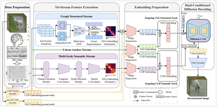
Figure 1: Schematic of TDE-Net. The diagram shows the raw EEG anchor, the sample-specific functional graph stream, the semantic temporal stream, dual-space mapping to VAE and CLIP, weighted fusion, and dual-conditioned Stable UnCLIP decoding. Tensor dimensions are indicated where applicable. Please click here to view a larger version of this figure.
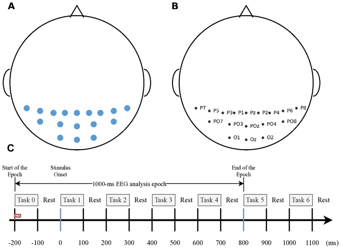
Figure 2: EEG electrode selection and experimental timing. (A) Spatial distribution of the selected 17 parieto-occipital electrodes from the original 64-channel acquisition. (B) Electrode labels: Pz, P3, P7, O1, Oz, O2, P4, P8, P1, P5, PO7, PO3, POz, PO4, PO8, P6, and P2. (C) Schematic of the RSVP timing and EEG epoch definition. In the schematic, “Task” denotes an image-presentation interval, whereas “Rest” denotes the inter-image interval; the numbered Task blocks indicate successive presentation intervals rather than different experimental conditions. Each image was presented for 100 ms with a 200-ms stimulus-onset asynchrony. The EEG epoch extended from -200 to 800 ms relative to stimulus onset, corresponding to a 1000-ms EEG analysis epoch. Please click here to view a larger version of this figure.
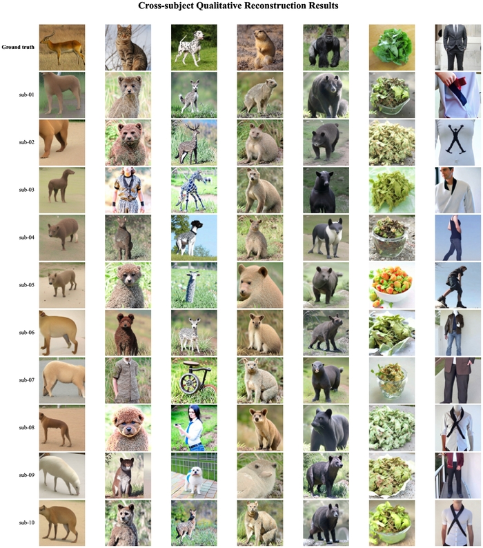
Figure 3: Cross-subject qualitative reconstruction results for seven held-out image conditions. The same zero-based condition indices (1, 32, 62, 86, 87, 108, and 175) are used for sub-01 through sub-10. The top row shows the corresponding ground-truth image samples from the THINGS-EEG2 test set, whose images were drawn from the THINGS image database34, whereas the remaining rows show TDE-Net reconstructions for each subject. The figure illustrates common semantic content and subject-level variation; quantitative cross-subject results are reported in Table 3. Please click here to view a larger version of this figure.
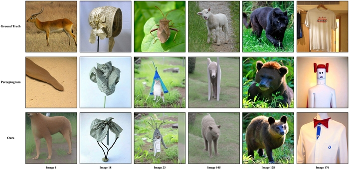
Figure 4: Qualitative reconstruction comparison for six specified sub-01 test conditions. Rows show the ground-truth stimulus, a comparator reconstruction generated by the local implementation, and the TDE-Net reconstruction; columns correspond to individual condition indices. Ground-truth image samples were drawn from the THINGS image database34. Please click here to view a larger version of this figure.
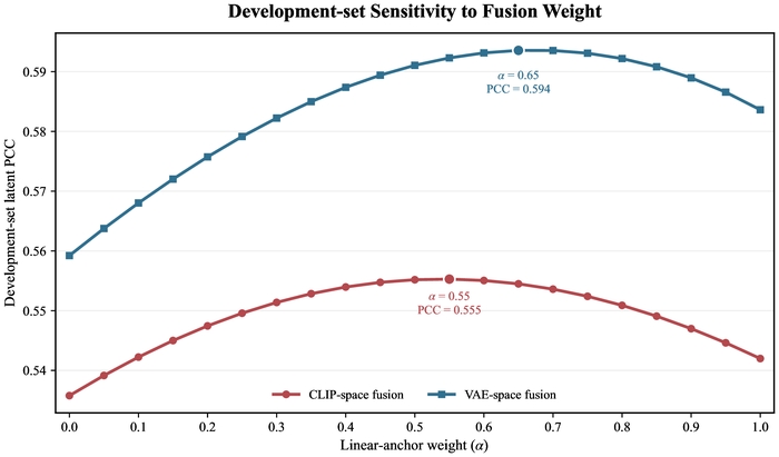
Figure 5: Development-set sensitivity of latent-fusion weights. The horizontal axis denotes the linear-anchor weight α, the complementary stream weight is 1 - α, and the vertical axis denotes development-set latent PCC. Candidate values range from 0.00 to 1.00 in increments of 0.05. CLIP- and VAE-space weights are selected independently by the maximum equally weighted mean subject-level PCC across 10 subjects, yielding αCLIP = 0.55 and αVAE = 0.65. PCC, Pearson correlation coefficient. Please click here to view a larger version of this figure.
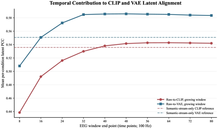
Figure 6: Temporal-window analysis of latent alignment in sub-01 (n = 200 held-out conditions). Solid curves show mean sample-wise PCC for raw-to-CLIP and raw-to-VAE ridge predictions as the EEG window endpoint expands from 8 to 80 time points at 100 Hz. Dashed lines indicate full-window semantic-stream-only CLIP and VAE reference values. PCC, Pearson correlation coefficient. Please click here to view a larger version of this figure.
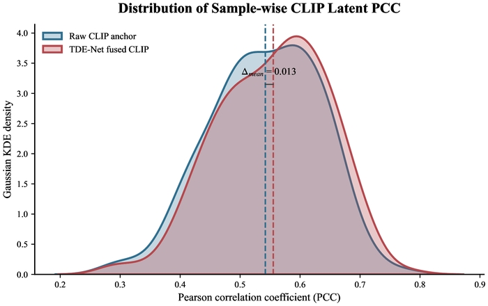
Figure 7: Distribution of sample-wise CLIP latent alignment in sub-01 (n = 200 held-out conditions). Curves are Gaussian kernel density estimates with Scott's bandwidth for the raw CLIP anchor and the frozen TDE-Net-fused CLIP prediction. Vertical dashed lines denote sample means, and the annotation indicates their difference. PCC, Pearson correlation coefficient; KDE, kernel density estimate. Please click here to view a larger version of this figure.
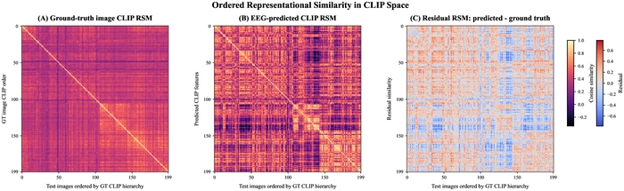
Figure 8: Ordered representational similarity in CLIP space for sub-01 (n = 200 held-out conditions). (A) Cosine-similarity RSM of L2-normalized ground-truth image CLIP embeddings. (B) Cosine-similarity RSM of fused EEG-predicted CLIP embeddings, displayed using the same ordering and color scale as panel A. (C) Residual RSM, calculated as predicted minus ground truth, displayed on a symmetric scale defined by the maximum absolute residual. Ordering is obtained by Euclidean distance and Ward linkage of ground-truth CLIP embeddings. RSM, representational similarity matrix. Please click here to view a larger version of this figure.
| Component | Parameter | Setting |
| Data and preprocessing | Dataset partition | 16,540 training and 200 held-out test conditions; 90%/10% fitting/development split (seed 42) |
| EEG input | 17 parieto-occipital channels; 0-800 ms; 100 Hz; 80 time points | |
| Spectral representation | 80-point FFT; 40 positive-frequency bins; 0-50 Hz log-amplitude spectrum | |
| Structural stream | Graph construction | Sample-specific absolute Pearson correlation; weighted top-k = 4 neighbors per node; symmetrization and self-loops |
| GCN architecture | 5 layers; 80 hidden units; ReLU; dropout 0.3; symmetric degree normalization; mean pooling | |
| Contrastive objective | 80-dimensional projection head; InfoNCE temperature τ = 0.5 | |
| Training | Adam; learning rate 5 × 10⁻⁴; batch size 32; 20 epochs; cosine annealing; minimum learning rate 10⁻⁶; seed 42 | |
| Semantic stream | Architecture | Temporal kernels 5/15/31; depth 9; 24 feature channels; dropout 0.5; output dimension 1,024 |
| Training | AdamW; learning rate 5 × 10⁻⁴; weight decay 0.01; batch size 64; 50 epochs; cosine annealing; minimum learning rate 10⁻⁶; seed 42 | |
| Latent mapping | Ridge regression | Intercept fitted; maximum iterations 50,000; inputs standardized using fitting-partition statistics |
| Regularization | CLIP penalty λ = 1,000; raw VAE penalty λ = 0; structural VAE penalty λ = 1,000 | |
| Target dimensions | CLIP: 1,024; VAE: 36,864 | |
| Fusion and decoding | Fusion weights | CLIP anchor weight α = 0.55; VAE anchor weight α = 0.65; selected on development data and fixed before testing |
| Diffusion model | sd2-community/stable-diffusion-2-1-unclip; structural scale γ = 0.02; diffusion timesteps T = 1,000 | |
| Sampling | 20 denoising steps; guidance scale 7.5; diffusion seed 0 |
Table 1: Consolidated parameter summary for TDE-Net. The table lists the data partition, preprocessing, functional adjacency construction, graph and semantic encoder settings, latent-mapping penalties, fusion weights, and diffusion-decoding settings used throughout the reported experiments.
| Method | PixCorr | SSIM | AlexNet(2) | AlexNet(5) | Inception | CLIP | EffNet | SwAV |
| Baseline | 0.141 | 0.321 | 0.823 | 0.878 | 0.704 | 0.739 | 0.898 | 0.564 |
| EEGImageDecode | - | 0.345 | 0.776 | 0.866 | 0.734 | 0.786 | - | 0.582 |
| Perceptogram (unCLIP) | 0.223 | 0.370 | 0.875 | 0.915 | 0.749 | 0.806 | 0.870 | 0.530 |
| TDE-Net (Ours) | 0.253 ± 0.014 | 0.339 ± 0.003 | 0.878 ± 0.012 | 0.915 ± 0.012 | 0.761 ± 0.021 | 0.814 ± 0.007 | 0.829 ± 0.012 | 0.509 ± 0.010 |
Table 2: Quantitative reconstruction results. The comparison methods, internal convolutional-attention Baseline, and TDE-Net were evaluated within a common experimental framework using the same THINGS-EEG2 partition, 17-channel input, preprocessing, held-out test conditions, and metric definitions, while retaining method-specific architectures. The present model is summarized as mean ± SD across 10 subjects. PixCorr, SSIM, AlexNet Layer 2, AlexNet Layer 5, Inception-v3, and CLIP are higher-is-better measures; EffNet and SwAV are correlation distances, for which lower is better. The CLIP column reports pairwise identification accuracy using the OpenAI CLIP ViT-L/14 model.
| Subject | PixCorr | SSIM | AlexNet L2 | AlexNet L5 | Inception | CLIP | EffNet | SwAV |
| sub-01 | 0.2260 | 0.3361 | 0.8831 | 0.9203 | 0.7533 | 0.8120 | 0.8567 | 0.5285 |
| sub-02 | 0.2488 | 0.3378 | 0.8699 | 0.9053 | 0.7268 | 0.8074 | 0.8335 | 0.5167 |
| sub-03 | 0.2564 | 0.3397 | 0.8728 | 0.9070 | 0.7658 | 0.8143 | 0.8268 | 0.5096 |
| sub-04 | 0.2420 | 0.3356 | 0.8598 | 0.9034 | 0.7854 | 0.8112 | 0.8255 | 0.5091 |
| sub-05 | 0.2499 | 0.3385 | 0.8760 | 0.8963 | 0.7251 | 0.8016 | 0.8394 | 0.5189 |
| sub-06 | 0.2621 | 0.3395 | 0.8910 | 0.9331 | 0.7818 | 0.8215 | 0.8202 | 0.5009 |
| sub-07 | 0.2489 | 0.3378 | 0.8643 | 0.9185 | 0.7704 | 0.8200 | 0.8222 | 0.5017 |
| sub-08 | 0.2786 | 0.3425 | 0.8951 | 0.9216 | 0.7524 | 0.8245 | 0.8214 | 0.5010 |
| sub-09 | 0.2609 | 0.3370 | 0.8775 | 0.9238 | 0.7662 | 0.8055 | 0.8250 | 0.5009 |
| sub-10 | 0.2571 | 0.3433 | 0.8871 | 0.9240 | 0.7792 | 0.8175 | 0.8140 | 0.4977 |
| Mean | 0.2531 | 0.3388 | 0.8777 | 0.9153 | 0.7606 | 0.8135 | 0.8285 | 0.5085 |
| Mean ± SD | 0.2531 ± 0.0138 | 0.3388 ± 0.0025 | 0.8777 ± 0.0115 | 0.9153 ± 0.0116 | 0.7606 ± 0.0213 | 0.8135 ± 0.0074 | 0.8285 ± 0.0122 | 0.5085 ± 0.0101 |
| 95% CI | 0.2432-0.2630 | 0.3370-0.3406 | 0.8695-0.8859 | 0.9070-0.9236 | 0.7454-0.7759 | 0.8082-0.8189 | 0.8198-0.8372 | 0.5013-0.5157 |
Table 3: Cross-subject quantitative results for TDE-Net. Each subject contributes 200 held-out test conditions. The table reports the eight metrics for sub-01 through sub-10, followed by the across-subject mean, sample SD, and 95% CI. CLIP denotes OpenAI CLIP ViT-L/14 pairwise identification accuracy; EffNet and SwAV are lower-is-better correlation distances.
| Method | PixCorr | SSIM | AlexNet(2) | AlexNet(5) | Inception | CLIP | EffNet | SwAV |
| Linear Anchor | 0.2157 | 0.3309 | 0.8891 | 0.9128 | 0.7493 | 0.7967 | 0.8683 | 0.5394 |
| Linear + Struct-Stream | 0.2318 | 0.3393 | 0.8861 | 0.9319 | 0.7439 | 0.7996 | 0.8657 | 0.5359 |
| Linear + Sem-Stream | 0.2372 | 0.3382 | 0.8879 | 0.9228 | 0.7447 | 0.8026 | 0.8655 | 0.5307 |
| TDE-Net (Ours) | 0.2531 | 0.3388 | 0.8777 | 0.9153 | 0.7607 | 0.8135 | 0.8285 | 0.5085 |
Table 4: Ablation results reported as across-subject mean values under the evaluation procedure described in Protocol Section 6. The Linear Anchor is a locally evaluated internal direct ridge-mapping reference; the structural, semantic, and complete configurations use the same condition indices and metric definitions. PixCorr, SSIM, AlexNet Layer 2, AlexNet Layer 5, Inception-v3, and CLIP are higher-is-better measures; EffNet and SwAV are lower-is-better correlation distances. Values are shown to three decimal places.
Supplementary Figure 1: Representative reconstruction cases spanning the CLIP-agreement range for sub-01. The 200 held-out conditions are ranked by cosine similarity between fused EEG-predicted and ground-truth CLIP embeddings; six best, six median, and six worst cases are shown. Each column pairs a ground-truth image sample from the THINGS-EEG2 test set with its TDE-Net reconstruction. The ground-truth images were drawn from the THINGS image database34. Please click here to download this file.
Supplementary Figure 2: Joint visualization of ground-truth and EEG-predicted CLIP representations in sub-01 (n = 200 conditions per representation). (A) Ground-truth CLIP representations. (B) EEG-predicted CLIP representations. Colors denote five k-means clusters fitted to L2-normalized ground-truth CLIP embeddings (k = 5, n_init = 50, seed = 7). The clusters are data-driven groups and do not correspond to predefined semantic categories. Ground-truth and predicted embeddings are concatenated, reduced to 50 dimensions by PCA, and jointly projected by t-SNE (perplexity = 28, learning rate = auto, Euclidean metric, seed = 12). PCA, principal component analysis; t-SNE, t-distributed stochastic neighbor embedding. Please click here to download this file.
Supplementary Figure 3: EEG patterns grouped by broad image-concept category for sub-01. Concepts are assigned to Animals, Food/plant-related concepts, or Other objects. Within each category, rows follow Ward's hierarchical ordering of whitened ground-truth CLIP embeddings and are uniformly sampled to at most 30 concepts for legibility. The columns show 17 EEG channels, with 80 time points per channel. The color scale (-1 to 1) represents clipped, normalized whitened EEG amplitude. Please click here to download this file.
Supplementary Figure 4: Semantic-stream scalp-channel attention topography. Colors show normalized relative magnitudes of learned channel-weight parameters across the selected 17 electrodes in a standard 10–20 scalp projection; electrode dots and labels identify measurement positions. The scale ranges from 0 to 1 and summarizes the model's learned relative channel weighting. Please click here to download this file.
ディスカッション
本研究では、EEGの前処理、構造的および意味的表現学習、CLIP/VAE潜在空間マッピング、融合、および拡散デコーディングを分離したモジュール式計算ワークフローを提示します。この段階的な構成により、生成された画像とは別に中間出力を個別に検討することが可能となり、コンパクトなEEGエンコーダーからクロスモーダルおよび拡散ベースの再構成手法へと至る広範な進展の流れに従っています6,11,12,13,14,15,16,,17,18,19,20,21,22。被験者間分析では、10名の被験者を対象としたホールドアウト評価において、被験者レベルの値とともに、被験者間の平均値およびサンプルSDを報告します。表4に示した段階的なアブレーション解析と併せて、この分析により、報告したパイプラインにおけるストリーム固有の効果と被験者間の変動を定量化します。
重要な手順とトラブルシューティング
最も重要な実装上の制御項目は、パーティションの分離、一貫した正規化、条件インデックスの保持、および個別のCLIP/VAEマッピングである。融合ウェイトは開発条件に基づいて選択し、テスト再構成の前に固定しなければならない。性能が予想よりも低い場合は、まずアレイの順序と次元を確認し、次に、生データおよびブランチ固有の潜在的PCC、融合メタデータ、および画像レベルの指標出力を検査する。潜在的アライメントの失敗は上流のマッピングの問題を示し、一方で潜在変数が安定しているにもかかわらず画像が変動する場合は、確率的またはデコーダー依存の挙動を反映している可能性がある14,21,22,29。
電極モンタージュ、サンプリングレート、または時間窓を変更する場合、グラフ構築、スペクトル特徴、および時間カーネルにも対応する変更を加える必要があります。単一のスコアではピクセル忠実度、構造、およびオブジェクトレベルの一致をすべて捉えることはできないため、再構成の品質は、補完的な低レベル指標および意味的指標を用いて評価する必要があります。6,11,21,22,23ここで使用されるCLIPの指標はペアごとの識別精度ですが、一方 図7 および 図 8 潜在レベルのPCCを使用してください。これらの量は互換性がありません。
TDE-Netのモジュール構成は、相補的なEEG表現が視覚再構成の構造的および意味的な側面にどのように異なる寄与をするかを検証するための枠組みを提供します。このアプローチにより、最終的な再構成画像のみに頼ることなく、EEG特徴表現、潜在ターゲット、および生成デコーダーの体系的な比較が可能になります。代替アプローチとしては、直接的な線形EEG-潜在マッピング、シングルストリームの畳み込みまたはアテンションベースのエンコーダー、グラフベースの表現、およびエンドツーエンドのニューラルデコードフレームワークなどが挙げられます6,7,8,9,10,11,17,18,19,20,21,22。本ワークフローは、視覚知覚デコーディング、神経表現解析、および非侵襲的ブレイン・コンピューター・インターフェースに関する研究において特に有用であり、中間的なEEG-潜在予測を分離することで、どの構成要素が再構成性能に寄与しているかを特徴付けるのに役立ちます。
限界事項
主な限界としては、THINGS-EEG2 RSVP取得の固定、選択された17個の頭頂・後頭チャンネル、被験者固有のマッピング、単一の拡散デコーダー、および定性的な解釈可能性分析が挙げられる21,22,23。10名の被験者のサマリーはデータセット内の被験者間変動に対処しているが、データセット間またはパラダイム間の転移を確立するものではない。生成された画像には、EEG入力によって裏付けられていない尤もらしい詳細が含まれる可能性があり、RSM、t-SNE、EEGパターン、およびアテンションビューは因果的な神経メカニズムを立証するものではない。段階的なアブレーション解析は、共通のraw EEGアンカー、潜在ターゲット、拡散デコーダー、および評価プロトコルの下での、構造ストリーム、意味ストリーム、およびデュアルスペース融合の寄与を特徴づけている。
今後の方向性
これらの制約の下で、本結果は、拡散デコードを行う前に、相補的なEEG表現を個別のセマンティック空間および画像潜在空間で評価することを支持しています。今後の研究では、独立したデータセット、被験者への適応、不確実性の推定、代替的なチャネル配置、およびサポートされていない視覚的詳細をより強力に制御したデコーダーを検証する必要があります14,15,16,17,18,19,20,21,22,23。現在の知見をより広範な神経科学やブレイン・コンピュータ・インターフェースの環境に展開する前に、このような研究が必要となります。
結論:
TDE-Netは、生のEEGアンカーを構造的および意味的なEEG表現と組み合わせ、それらをVAEおよびCLIPの潜在空間と個別に整合させ、拡散デコーディングの前に得られた予測を統合します。10名のTHINGS-EEG2参加者において、再構成された画像は、閲覧した刺激との間で測定可能なピクセルレベル、構造的、および意味的な対応関係を保持しており、段階的なアブレーション解析により、構造ストリーム、意味ストリーム、およびデュアルスペース融合の効果が区別されました。中間EEG特徴量、潜在予測、融合出力、および最終的な再構成結果を提示することで、本プロトコルは、EEGに基づく視覚再構成を調査し、独立したデータセットや取得設定への将来的な拡張を評価するための再現可能なフレームワークを提供します。
開示事項
著者らは、本研究に影響を及ぼす可能性のある競合する金銭的利益や個人的関係がないことを宣言します。また、原稿の作成、コードの記述、データ解析、および図の作成において、生成AIツールは一切使用されなかったことを宣言します。
謝辞
本研究は、中国国家自然科学基金(助成金番号 62433002 および 62476014)、国家科学技術重大プロジェクト(No. 2021ZD0113703)、北京市社会科学基金年次計画プロジェクト(No. 23GLB014)、北京市機関ハイレベル革新チーム構築・支援プロジェクト(助成金番号 BPHR20220104)、および北京学者プログラム(助成金番号 099)より資金提供を受けて実施されました。
材料
| 名前 | 会社 | カタログ番号 | コメント |
|---|---|---|---|
| 加速させる | Hugging Face | 0.30.1 | 拡散パイプラインのデバイス管理; https://github.com/huggingface/accelerate |
| CLIP ViT-L/14 | OpenAI | ViT-L/14; openai-clip 1.0.1 | セマンティックターゲットおよびCLIPペア識別に使用される画像特徴エンコーダー;https://github.com/openai/CLIP |
| ディフューザー | Hugging Face | 0.32.2 | Stable UnCLIPパイプラインの実装;https://github.com/huggingface/diffusers |
| Matplotlib | Matplotlib開発チーム | 3.10.6 | 科学的な図の作成; https://matplotlib.org/ |
| MNE-Python | MNE開発者 | 1.11.0 | 標準的な10-20法電極配置および頭皮チャネルトポグラフィー;https://mne.tools/ |
| NumPy | NumPy開発者 | 2.3.4 | EEGアレイ、潜在埋め込み、融合、および指標集計; https://numpy.org/ |
| NVIDIA GeForce RTX 4070 Laptop GPU | NVIDIA | 8 GB; ドライバー 595.97 | ローカルエンコーダーのトレーニングおよび拡散再構成に使用されたGPU。 |
| ピロー | Python Imaging Library フォーク | 11.1.0 | 画像の読み込み、リサイズ、およびエクスポート; https://python-pillow.org/ |
| Python | Python Software Foundation | 3.12.12 | 主要ランタイム環境; https://www.python.org/ |
| PyTorch | PyTorch Foundation | 2.9.1+cu128 | EEGエンコーダのトレーニングとニューラルネットワークによる推論; https://pytorch.org/ |
| scikit-image | scikit-image 開発者 | 0.25.2 | SSIMおよび画像処理ユーティリティ; https://scikit-image.org/ |
| scikit-learn | scikit-learn 開発者 | 1.7.2 | リッジ回帰、k-means、PCA、t-SNE; https://scikit-learn.org/ |
| SciPy | SciPy開発者 | 1.16.3 | 相関、統計的距離、および階層的クラスタリング; https://scipy.org/ |
| Seaborn | Seaborn開発者 | 0.13.2 | ガウスカーネル密度可視化; https://seaborn.pydata.org/ |
| 意味ストリームEEGエンコーダー | TDE-Net著者;LMDA-Netより改変 | リポジトリコミット c99325d | マルチスケール時間的意味表現。実装およびチェックポイントのメタデータはコードリポジトリで提供されています。 |
| Stable Diffusion 2.1 UnCLIP | Stability AI / SD2 コミュニティ | sd2-community/stable-diffusion-2-1-unclip | 凍結拡散デコーダー; https://huggingface.co/sd2-community/stable-diffusion-2-1-unclip |
| 構造ストリームEEGエンコーダー | TDE-Netの著者 | リポジトリコミット c99325d | 自己教師ありグラフ表現。生のEEGおよびグラフ特徴量は、VAE空間の構造的マッピングのためだけに結合される。 |
| TDE-Netのアライメント、統合、評価、および可視化スクリプト | Yuan-ui198 | コミット c99325d7f9e090ddd7cd581 申し訳ございませんが、翻訳対象となるソーステキストが提供されていません。翻訳が必要なテキストを入力してください。 | https://github.com/Yuan-ui198/TDE-Net/tree/c99325d7f9e0 (提供されたテキストがありません。翻訳するソーステキストを入力してください。) |
| THINGSデータベース | Hebartら | doi:10.1371/journal.pone.0223792 | 自然主義的物体刺激ソース; https://things-initiative.org/ |
| THINGS-EEG2データセット | Giffordら | doi:10.1016/j.neuroimage.2022.119754 | 10名の被験者から得られた64チャンネルEEG;本研究では17の頭頂後頭部チャンネルを選択;https://osf.io/anp5v/ |
| timm | Ross Wightmanおよび共同研究者 | 1.0.22 | 特徴評価に使用される事前学習済みビジョンモデル・ユーティリティ; https://github.com/huggingface/pytorch-image-models |
| torchvision | PyTorch Foundation | 0.24.1+cu128 | AlexNet、Inception-v3、およびEfficientNetの評価バックボーン; https://pytorch.org/vision/ |
| tqdm | tqdm 開発者 | 4.67.1 | 特徴抽出、再構成、および評価の進捗レポート;https://tqdm.github.io/ |
| トランスフォーマー | Hugging Face | 4.37.2 | 事前学習済みモデルコンポーネントのインターフェース; https://github.com/huggingface/transformers |
参考文献
- Shen G, Horikawa T, Majima K, Kamitani Y. Deep image reconstruction from human brain activity. PLoS Comput Biol. 2019;15(1):e1006633. doi:10.1371/journal.pcbi.1006633.
- Chen Z, Qing J, Xiang T, Yue W, Zhou JH. Seeing beyond the brain: conditional diffusion model with sparse masked modeling for vision decoding. In: Proceedings of the IEEE/CVF Conference on Computer Vision and Pattern Recognition. 2023. p. 22710-22720. Available from: https://openaccess.thecvf.com/content/CVPR2023/html/Chen_Seeing_Beyond_the_Brain_Conditional_Diffusion_Model_With
_Sparse_Masked_Modeling_CVPR_2023_paper.html - Takagi Y, Nishimoto S. High-resolution image reconstruction with latent diffusion models from human brain activity. In: Proceedings of the IEEE/CVF Conference on Computer Vision and Pattern Recognition. 2023. p. 14453-14463. Available from: https://openaccess.thecvf.com/content/CVPR2023/html/Takagi_High-Resolution_Image_Reconstruction_With_Latent_Diffusion_Models_
From_Human_Brain_CVPR_2023_paper.html - Scotti PS et al. Reconstructing the mind's eye: fMRI-to-image with contrastive learning and diffusion priors. Adv Neural Inf Process Syst. 2023;36:24705-24728. doi:10.52202/075280-1073.
- Geman S, Bienenstock E, Doursat R. Neural networks and the bias/variance dilemma. Neural Comput. 1992;4(1):1-58. doi:10.1162/neco.1992.4.1.1.
- Lawhern VJ et al. EEGNet: a compact convolutional neural network for EEG-based brain-computer interfaces. J Neural Eng. 2018;15(5):056013. doi:10.1088/1741-2552/aace8c.
- Kostas D, Aroca-Ouellette S, Rudzicz F. BENDR: using transformers and a contrastive self-supervised learning task to learn from massive amounts of EEG data. Front Hum Neurosci. 2021;15:653659. doi:10.3389/fnhum.2021.653659.
- Song Y, Zheng Q, Liu B, Gao X. EEG Conformer: convolutional transformer for EEG decoding and visualization. IEEE Trans Neural Syst Rehabil Eng. 2023;31:710-719. doi:10.1109/TNSRE.2022.3230250.
- Cui CM et al. "Pre-Train, Prompt" framework to boost graph neural networks performance in EEG analysis. IEEE J Biomed Health Inform. 2025;29(7):4847-4860. doi:10.1109/JBHI.2025.3541058.
- Meng X, Qiu S, Wan S, Cheng K, Cui L. A motor imagery EEG signal classification algorithm based on recurrence plot convolution neural network. Pattern Recognit Lett. 2021;146:134-141. doi:10.1016/j.patrec.2021.03.023.
- Miao Z, Zhao M, Zhang X, Ming D. LMDA-Net: a lightweight multi-dimensional attention network for general EEG-based brain-computer interfaces. Neuroimage. 2023;276:120209. doi:10.1016/j.neuroimage.2023.120209.
- Zhang S, Tang C, Guan C. Visual-to-EEG cross-modal knowledge distillation for continuous emotion recognition. Pattern Recognit. 2022;130:108833. doi:10.1016/j.patcog.2022.108833.
- Palazzo S et al. Decoding brain representations by multimodal learning of neural activity and visual features. IEEE Trans Pattern Anal Mach Intell. 2021;43(11):3833-3849. doi:10.1109/TPAMI.2020.2995909.
- Rombach R, Blattmann A, Lorenz D, Esser P, Ommer B. High-resolution image synthesis with latent diffusion models. In: Proceedings of the IEEE/CVF Conference on Computer Vision and Pattern Recognition. 2022. p. 10684-10695. Available from: https://openaccess.thecvf.com/content/CVPR2022/html/Rombach_High-Resolution_Image_Synthesis_With_Latent_Diffusion_Models_CVPR
_2022_paper.html - Radford A et al. Learning transferable visual models from natural language supervision. In: Proceedings of the 38th International Conference on Machine Learning. PMLR. 2021;139:8748-8763. Available from: https://proceedings.mlr.press/v139/radford21a.html
- Bai Y et al. DreamDiffusion: high-quality EEG-to-image generation with temporal masked signal modeling and CLIP alignment. In: Computer Vision - ECCV 2024. Cham: Springer; 2024. p. 472-488. doi:10.1007/978-3-031-72751-1_27.
- Cao X, Gong P, Zhang L, Zhang D. EEG-CLIP: a transformer-based framework for EEG-guided image generation. Neural Netw. 2026;194:108167. doi:10.1016/j.neunet.2025.108167.
- Liu Y et al. FSDBN: foreground-aware EEG-visual alignment via dynamic brain networks. arXiv [Preprint]. 2026. Available from: https://arxiv.org/abs/2607.18344
- Yin F, Zheng C, Gong P, Guan D, Zhu Q. Neural visual decoding via cognitive-guided adaptive blurring and information-constrained alignment. arXiv [Preprint]. 2026. Available from: https://arxiv.org/abs/2605.16418
- Liu J, Gong P, Zheng C, Liu Y, Zhu Q. Multi-level bidirectional biomimetic learning for EEG-based visual decoding. arXiv [Preprint]. 2026. Available from: https://arxiv.org/abs/2605.04680
- Fei T et al. Perceptogram: reconstructing visual percepts and presumptive electrode preference from EEG. arXiv [Preprint]. 2024. Available from: https://arxiv.org/abs/2404.01250
- Li D, Wei C, Li S, Zou J, Liu Q. Visual decoding and reconstruction via EEG embeddings with guided diffusion. Adv Neural Inf Process Syst. 2024;37:102822-102864. doi:10.52202/079017-3266.
- Gifford AT, Dwivedi K, Roig G, Cichy RM. A large and rich EEG dataset for modeling human visual object recognition. Neuroimage. 2022;264:119754. doi:10.1016/j.neuroimage.2022.119754.
- Kipf TN, Welling M. Semi-supervised classification with graph convolutional networks. In: International Conference on Learning Representations. 2017. Available from: https://openreview.net/forum?id=SJU4ayYgl
- Chen T, Kornblith S, Norouzi M, Hinton G. A simple framework for contrastive learning of visual representations. In: Proceedings of the 37th International Conference on Machine Learning. PMLR. 2020;119:1597-1607. Available from: https://proceedings.mlr.press/v119/chen20j.html
- Ramoser H, Muller-Gerking J, Pfurtscheller G. Optimal spatial filtering of single trial EEG during imagined hand movement. IEEE Trans Rehabil Eng. 2000;8(4):441-446. doi:10.1109/86.895946.
- Bai S, Kolter JZ, Koltun V. An empirical evaluation of generic convolutional and recurrent networks for sequence modeling. arXiv [Preprint]. 2018. Available from: https://arxiv.org/abs/1803.01271
- Woo S, Park J, Lee JY, Kweon IS. CBAM: convolutional block attention module. In: European
Conference on Computer Vision. Cham: Springer; 2018. p. 3-19. Available from:
https://doi.org/10.1007/978-3-030-01234-2_1 - Hoerl AE, Kennard RW. Ridge regression: biased estimation for nonorthogonal problems. Technometrics. 1970;12(1):55-67. doi:10.1080/00401706.1970.10488634.
- Zhou ZH. Ensemble Methods: Foundations and Algorithms. Boca Raton: Chapman and Hall/CRC; 2012.
- Ho J, Jain A, Abbeel P. Denoising diffusion probabilistic models. Adv Neural Inf Process Syst. 2020;33:6840-6851. Available from: https://proceedings.neurips.cc/paper/2020/hash/4c5bcfec8584af0d967f1ab10179ca4b-Abstract.html
- Ho J, Salimans T. Classifier-free diffusion guidance. arXiv [Preprint]. 2022. Available from: https://arxiv.org/abs/2207.12598
- Kingma DP, Welling M. Auto-encoding variational Bayes. In: International Conference on Learning Representations. 2014. Available from: https://openreview.net/forum?id=33X9fd2-9FyZd
- Hebart MN et al. THINGS: a database of 1,854 object concepts and more than 26,000 naturalistic object images. PLoS One. 2019;14(10):e0223792. doi:10.1371/journal.pone.0223792.
再版と許可
この記事は公開されました
動画は近日公開