본 프로토콜에서는 상보적인 EEG 표현, 이중 공간 시각적 정렬 및 확산 디코딩을 결합한 EEG-이미지 재구성 프레임워크인 Tri-stream Disentangled Network (TDE-Net)를 제시합니다.
방법 논문
THINGS-EEG2 데이터셋의 뇌파 기반 이미지 재구성을 위한 적응형 듀얼 공간 융합 기반의 삼중 스트림 얽힘 해제 네트워크
이 논문에서
요약
초록
비침습적 뇌전도(EEG)로부터 시각 자극을 재구성하려면 제한된 공간적 샘플링에도 불구하고 짧고 노이즈가 많은 신경 반응을 의미 있는 시각적 표현으로 매핑해야 합니다. 기존의 EEG-to-image 방식들은 다양한 신경 표현과 생성 전략을 채택하고 있으며, 이에 따라 구조적 기여분과 의미론적 기여분을 분리하는 재현 가능한 워크플로우가 필요합니다. 본 프로토콜에서는 EEG 기반 이미지 재구성을 위한 계산 프레임워크인 Tri-stream Disentangled Network (TDE-Net)를 제시합니다. 이 프로토콜은 전처리된 THINGS-EEG2 기록을 사용하며, EEG 정보를 raw EEG 앵커, 샘플별 기능적 그래프 스트림, 그리고 다중 스케일 시간적 의미 스트림으로 구성합니다. 그래프 스트림은 그래프 컨볼루션과 시행 간 대조 학습(cross-trial contrastive learning)을 통해 EEG 채널 간의 주파수 영역 관계를 포착하며, 의미 스트림은 적응형 공간 가중치와 다중 스케일 시간적 컨볼루션을 통해 과제 관련 특징을 추출합니다. 구조적 특징과 의미론적 특징은 각각 변분 오토인코더(VAE) 및 Contrastive Language-Image Pre-training (CLIP) 잠재 공간으로 매핑되고, 개발 세트에서 선택된 융합 가중치를 사용하여 결합된 후 Stable UnCLIP을 통해 디코딩됩니다. 10명의 피험자를 대상으로 한 실험에서 TDE-Net은 평균 0.8135의 CLIP 쌍별 식별 정확도를 달성하였으며, 보완적 지표들을 통해 구조 및 특징 공간의 대응 관계를 입증하였습니다. 어블레이션(ablation) 및 표현 수준 분석을 통해 개별 스트림의 기여도를 추가로 규명하였습니다. 본 프로토콜은 상호 보완적인 EEG 표현과 확산 기반 시각 재구성을 연구하기 위한 재현 가능한 프레임워크를 제공합니다.
서론
시각적 지각 해독은 뇌-컴퓨터 인터페이스(BCI)와 인지 신경과학의 다학제적 연구 분야입니다. 기능적 자기공명영상(fMRI)을 통해 실제에 가까운 이미지 재구성이 가능해졌으나1,2,3,4, 높은 비용과 제한된 휴대성, 혈역학적 지연으로 인해 일부 응용 분야에 제약이 있습니다. 뇌전도(EEG)는 상대적으로 접근 가능한 장비를 통해 밀리초 단위의 시간적 측정을 제공하지만, 낮은 신호 대 잡음비와 제한된 공간적 샘플링으로 인해 EEG 기반의 이미지 재구성이 어렵습니다.
방법의 복잡성은 일반적인 편향-분산 트레이드오프(bias-variance trade-off)5의 관점에서 해석되어야 합니다. 초기 시각적 디코딩 방법은 얕은 표현이나 선형 표현을 사용한 반면, 이후의 연구들은 콤팩트한 합성곱(convolutional), 그래프 기반 및 어텐션 기반 인코더를 도입하였습니다6,7,8,9,10,11. 교차 모달 정렬(Cross-modal alignment) 또한 다중 모달 특징 학습12,13에서 잠재 확산 모델(latent diffusion models) 및 대형 비전 인코더14,15,16로 발전해 왔습니다. 이러한 접근 방식들은 유용한 기준점(baseline)을 제시하지만, 입력 표현, 잠재 타겟 및 디코더가 서로 다르므로 결과는 각각의 실험 설정 내에서 해석되어야 합니다.
TDE-Net의 목적은 구조적 EEG 표현과 의미적 EEG 표현을 분리하고, 이를 상보적인 시각적 잠재 공간과 정렬하며, 확산 기반 이미지 재구성을 위해 이러한 예측값들을 통합하는 모듈형 EEG-이미지 재구성 프레임워크를 제공하는 것입니다. 최근의 EEG-시각 디코딩 연구에서는 EEG-CLIP17의 트랜스포머 기반 EEG 유도 생성, FSDBN18의 동적 뇌 네트워크를 이용한 전경 인식 정렬, 정보 제약 정렬을 통한 인지 유도 적응형 블러링19, 그리고 다층 양방향 생체 모방 학습20 등이 소개되었습니다. Perceptogram 및 EEG 임베딩 기반의 유도 확산을 포함한 관련 EEG-이미지 파이프라인들은 잠재 예측을 위한 추가적인 참고 자료를 제공합니다21,22. TDE-Net은 모델 구성 방식에서 차이가 있습니다. 즉, 원시 EEG 앵커, 샘플별 기능적 그래프 표현, 그리고 시간적 의미 표현을 명시적으로 분리한 후, 융합 전에 VAE 및 CLIP 공간으로 비대칭 정렬을 수행합니다. 이러한 구성은 잠재 공간 및 이미지 수준 분석을 통해 구조적 기여도와 의미적 기여도를 개별적으로 검토할 수 있게 합니다. 단일 표현 방식이나 직접 정렬된 EEG-이미지 접근 방식과 비교하여, 이 모듈형 설계는 구조적 및 의미적 경로를 분리하여 제공하고, 잠재 예측 과정에서 선형 EEG 참조를 유지하며, 어블레이션 분석 및 잠재 공간 분석을 통해 각 표현의 기여도를 독립적으로 평가할 수 있게 합니다.
TDE-Net은 쌍을 이루는 EEG 응답과 시각적 자극이 있고, 충분한 훈련 조건이 갖춰졌으며, 의미론적 재구성이 주된 목적인 짧은 자극 후 윈도우를 사용하는 실험을 위해 설계되었습니다. 이 모델의 단계별 구조는 특징 추출, 잠재 정렬, 융합 및 확산 디코딩에 대한 개별적인 검토를 지원합니다. 매우 작은 데이터셋이나 모델 복잡성의 최소화를 우선시하는 설정에는 선형 매핑이 적합하며, 대규모의 작업 특정 데이터셋과 실시간 배포가 가능한 경우에는 엔드투엔드 신경망 디코더가 더 선호될 수 있습니다.
본 프로토콜은 THINGS-EEG2 신속 순차 시각 제시(RSVP) 설정에서 제안된 구성의 성능을 평가합니다. 주요 기여 사항으로는 raw 선형 앵커, 샘플별 기능 그래프 스트림, 다중 스케일 시간적 의미 스트림으로 구성된 3-스트림 EEG 표현 체계가 포함됩니다. 이러한 상호 보완적인 표현들은 VAE 및 CLIP 잠재 공간으로 매핑되며, 해당 예측값들은 확산 디코딩 전에 결합됩니다. 이 프레임워크는 피험자 수준의 재구성 척도, 어블레이션 및 시간 윈도우 분석, 표현 수준의 시각화를 사용하여 THINGS-EEG2의 모든 피험자 10명을 대상으로 평가되었으며, 공간 주의력 맵은 두피 채널(지형적) 분석으로 해석되었습니다.
프로토콜
The protocol comprises six sequential stages: preparation of EEG trials and image latents; construction of the graph structural stream; training of the semantic EEG encoder; fitting of the CLIP/VAE mappings; fusion of the latent predictions, followed by image decoding; and evaluation of image-level and representation-level outcomes (Figure 1).
1. Prepare EEG trials and image embeddings
- Document the source cohort and acquisition protocol.
NOTE: The source cohort comprised 10 healthy adults (mean age 28.5 years, SD 4.0; eight female and two male) with normal or corrected-to-normal vision. Participants provided written informed consent, received monetary compensation, and completed the original protocol with approval from the ethics committee of the Department of Education and Psychology at Freie Universität Berlin, in accordance with the Declaration of Helsinki23.- Use the publicly available THINGS-EEG2 dataset as a secondary-analysis resource.
- Use the source partition of 1,654 training concepts and 200 non-overlapping test concepts drawn from THINGS, with the proportions of 27 higher-level categories balanced between partitions. Select ten natural-background images for each training concept and one image for each test concept, to yield 16,540 training conditions and 200 held-out test conditions.
NOTE: In the present study, the target-detection task used separate Buzz Lightyear catch images that were excluded from the present reconstruction analysis23. - Follow the timing of the original rapid serial visual presentation protocol when interpreting the epochs.
NOTE: Each sequence began with a 750 ms blank interval, followed by 20 centrally presented images. Each image subtended 7 degrees of visual angle, remained on screen for 100 ms, and had a 200 ms stimulus-onset asynchrony, corresponding to 5 images/s. A second 750 ms blank interval preceded a response period of up to 2 s, during which participants first blinked and then reported whether a target image had appeared. A central bull's-eye fixation target remained visible throughout the sequence23. - Account for the original recording-session structure when organizing the dataset. Use data from the four recording sessions completed by each participant, with each session comprising four test runs and 15 training runs of approximately 5 min each. Retain four repetitions for each training condition and 80 repetitions for each test condition, corresponding to 82,160 analyzed non-target image trials per participant23.
- Use the EEG data acquired with the original THINGS-EEG2 recording configuration. These recordings were acquired at 1,000 Hz using a 64-electrode EASYCAP arranged according to the international 10-10 system and a BrainVision actiCHamp amplifier, with Fz as the online reference and an online 0.1–100 Hz band-pass filter.
- Use the released preprocessed data, which were epoched from -200 to 800 ms relative to image onset, baseline-corrected using the prestimulus interval, downsampled to 100 Hz, restricted to 17 parieto-occipital channels, cleared of target trials, and subjected to multivariate noise normalization independently within each recording session23.
- Prepare EEG trial tensors
- Load the released preprocessed THINGS-EEG2 tensors for all 10 participants. From each source epoch, select the 0–800 ms post-stimulus interval and the 17 parieto-occipital channels, retaining the 100 Hz sampling rate to obtain 80 time points per trial. Preserve the source partition of 16,540 training image conditions and 200 held-out test image conditions for each participant23 (Figure 2).
- For graph-stream pre-training, retain the four independent training repetitions for each image condition and sample two repetitions to form a positive pair. For the raw and semantic streams, average the four training repetitions and average the 80 available test repetitions for each condition.
- Use the preprocessed THINGS-EEG2 tensors produced by the original MVNN pipeline; within each implemented feature extractor, apply the documented file-level Z-scoring before feature computation.
NOTE: This asymmetric use of repetitions is deliberate: repeated trials provide positive pairs for graph-stream contrastive pre-training, whereas the raw and semantic streams use condition-level averages for supervised mapping. The resulting design combines repetition-level invariance learning in the structural stream with condition-level latent prediction in the raw and semantic streams.
- Prepare paired image latents
- Use the 1,024-dimensional CLIP vision encoder and the VAE encoder associated with sd2-community/stable-diffusion-2-1-unclip to extract paired image targets. Resize VAE input images to 768 x 768 pixels, store the VAE posterior mode as a 36,864-dimensional vector (4 x 96 x 96), and preserve the image-condition order.
- Save three input forms: repeated-trial tensors for graph contrastive learning, averaged EEG tensors for the raw and semantic streams, and paired CLIP/VAE image latents for supervised mapping.
- Normalize and cache the inputs
- Cache the preprocessed EEG tensors, extracted graph and semantic features, and paired image latents with fixed condition ordering.
- During ridge mapping, estimate feature-wise standardization parameters from the training inputs and apply those parameters to the development and test inputs.
2. Construct the graph structural stream
- Construct the graph stream from repeated training trials and export node-level features after contrastive pre-training. Use the same graph construction rule for test feature extraction, without using test image latents during feature computation.
- Transform EEG trials into frequency-domain graph inputs
- Transform each trial with an 80-point fast Fourier transform (FFT) and retain the first 40 nonnegative-frequency bins, spanning 0 Hz–48.75 Hz at the 100 Hz sampling rate. Use the log-amplitude spectrum as a 17 x 40 node-feature matrix X. For each EEG sample, calculate C_ij = |corr(X_i, X_j)| between every pair of the 17 channel feature vectors.
- In each row, retain the diagonal self-correlation and the three strongest off-diagonal correlations (k = 4 retained entries including self), then symmetrize the retained matrix to define the sample-specific weighted functional adjacency A. Apply symmetric degree normalization before graph convolution.
- Use this construction during training and testing; electrode physical coordinates are not used to define a fixed graph.
NOTE: Retaining self-connectivity preserves each node's signal, whereas limiting cross-channel connections to 3 per row controls graph density prior to symmetrization. The frequency-domain representation provides a compact amplitude-based description for graph construction, but does not preserve phase or all fine-grained phase-locked ERP timing; those temporal aspects remain available in the raw anchor and semantic temporal streams.
- Aggregate electrode topology with spectral graph convolution
- Apply a five-layer graph convolutional network (GCN)24 with 80 hidden units per layer, ReLU activations, 0.3 dropout, symmetric degree normalization, and mean graph pooling.
- Use an 80-dimensional two-layer projection head for the contrastive objective, and export the 17 x 80 node-level representation for structural fusion. Apply spectral graph convolution to the input-dependent adjacency matrix; do not introduce a separate dynamic convolution operator.
- Train the graph stream with cross-trial contrastive learning
- Within the training partition, randomly select two repetitions from the same image condition as a positive pair and treat representations from other conditions in the batch as negatives. Optimize the InfoNCE contrastive objective25 with temperature τ = 0.5, batch size 32, Adam with learning rate 5 x 10⁻⁴, 20 epochs, cosine annealing to eta_min = 10–6, and random seed 42.
 (1)
(1) - Define cosine similarity in the contrastive objective and use the indicator function to identify paired repetitions. Keep the projection dimension at 80 and apply the same temperature to both directions of the contrastive loss.
- Within the training partition, randomly select two repetitions from the same image condition as a positive pair and treat representations from other conditions in the batch as negatives. Optimize the InfoNCE contrastive objective25 with temperature τ = 0.5, batch size 32, Adam with learning rate 5 x 10⁻⁴, 20 epochs, cosine annealing to eta_min = 10–6, and random seed 42.
- Export node-level graph features for early fusion
- Freeze the graph encoder after pre-training and export the 17-channel node features with 80 dimensions per node. Concatenate these features with the averaged raw EEG along the feature dimension to obtain the raw-plus-graph structural input for VAE mapping.
- Save the resulting raw-plus-graph feature tensor and use it only as the structural input to the VAE regression branch.
3. Train the semantic EEG encoder
- Train the semantic EEG encoder on the averaged 17-channel, 80-point EEG tensors.
- Optimize cosine embedding loss with AdamW (learning rate 5 x 10⁻⁴; weight decay 0.01), batch size 64, 50 epochs, cosine annealing to eta_min = 10–6, random seed 42, and a 1,024-dimensional output.
- Apply data-driven adaptive spatial filtering
- Apply a learnable tensor-product channel weighting operation to the input EEG tensor and expand the representation to a depth of 9. Treat this operation as a data-driven channel-weighting layer rather than an implementation of the classical Common Spatial Pattern (CSP) spatial filter26.
 (2)
(2) - Use the learned channel-weighting operation to produce nine feature maps, then pass them to the multi-scale temporal convolution block.
- Apply a learnable tensor-product channel weighting operation to the input EEG tensor and expand the representation to a depth of 9. Treat this operation as a data-driven channel-weighting layer rather than an implementation of the classical Common Spatial Pattern (CSP) spatial filter26.
- Model temporal receptive fields at multiple scales
- Apply three parallel temporal convolutions with kernel sizes 5, 15, and 31 samples, using same-length padding. Concatenate the three outputs to obtain 24 temporal feature channels and apply batch normalization and GELU activation.
 (3)
(3)
NOTE: The convolutions provide multi-scale temporal receptive fields within the broader temporal convolutional modeling framework27. - Use the three kernel sizes as multi-scale temporal filters; interpret their output as learned signal representations rather than as direct assignments to specific ERP components.
- Apply three parallel temporal convolutions with kernel sizes 5, 15, and 31 samples, using same-length padding. Concatenate the three outputs to obtain 24 temporal feature channels and apply batch normalization and GELU activation.
- Recalibrate task-relevant feature channels
- Apply depth attention with adaptive average pooling to the temporal dimension and a kernel-7 convolution followed by Softmax normalization, consistent with channel-recalibration principles28. Multiply the resulting attention weights element-wise with the multi-scale feature tensor.
 (4)
(4) - Use the attention output as the input to the spatial convolution block and do not interpret the learned weights as causal neural localization.
- Apply depth attention with adaptive average pooling to the temporal dimension and a kernel-7 convolution followed by Softmax normalization, consistent with channel-recalibration principles28. Multiply the resulting attention weights element-wise with the multi-scale feature tensor.
- Export the global semantic EEG feature
- Apply a 1 x 1 convolution followed by a depthwise convolution spanning the 17 electrode channels, batch normalization, GELU activation, average pooling with factor 2, and dropout p = 0.5. Flatten the result and project it to a 1,024-dimensional semantic feature vector.
- Save one 1,024-dimensional semantic feature vector for each averaged EEG sample.
4. Map EEG features to CLIP and VAE latent spaces
- Pair each EEG feature tensor with the image latent having the same condition index. Fit separate mappings for CLIP and VAE targets, and keep all image conditions in the training partition disjoint from those in the held-out test partition.
- Fit ridge regression29 with an intercept and a maximum of 50,000 iterations. Use λCLIP = 1,000 for the raw-to-CLIP and semantic-to-CLIP mappings, λVAE = 0 for the raw-to-VAE anchor, and λVAE, struct = 1,000 for the structural-stream-to-VAE mapping. Standardize mapping inputs using fit-partition statistics.
NOTE: The structural stream is the concatenation of raw EEG and graph features; the semantic stream contains the semantic encoder output without raw-feature concatenation. - Map structural features to the VAE latent space
- Fit the structural-stream-to-VAE ridge mapping with λVAE,struct = 1,000 and predict the 36,864-dimensional VAE latent. This branch receives the concatenated raw EEG and graph representations; it is the only nonlinear branch that explicitly concatenates raw features.
- Map semantic features to the CLIP latent space
- Fit the semantic-stream-to-CLIP ridge mapping with λCLIP = 1,000 and predict the 1,024-dimensional CLIP representation. The semantic input is not concatenated with raw EEG.
NOTE: In this article, λ denotes ridge regularization and α denotes a latent-fusion weight. - Assess latent-space alignment with sample-wise Pearson correlation coefficient (PCC). Use development conditions for fusion-weight selection and assess the 200 held-out test conditions only after the mappings and fusion weights have been frozen.
- Fit the semantic-stream-to-CLIP ridge mapping with λCLIP = 1,000 and predict the 1,024-dimensional CLIP representation. The semantic input is not concatenated with raw EEG.
5. Fuse latent predictions and run diffusion reconstruction
- Select αVAE and αCLIP using a condition-level development split derived only from the 16,540 training conditions. With random seed 42, use the same 90% fit indices and 10% development indices for all 10 subjects; the 200 held-out test conditions remain outside this procedure.
NOTE: The ridge penalties and structural preservation coefficient were fixed as configuration values before the final held-out evaluation and were not tuned against the 200 test conditions. - For each subject and each candidate α in {0.00, 0.05, ..., 1.00}, fit the target-supervised encoder and ridge mappings on the fit subset and calculate mean sample-wise latent PCC on the development subset.
- Average the subject-level PCC values with equal weight across the 10 subjects, and select CLIP- and VAE-space weights independently by the maximum cross-subject mean. Freeze both values before refitting the final training models and evaluating the held-out test conditions.
NOTE: This procedure selected αCLIP = 0.55 and αVAE = 0.65. - For the VAE space, define the fused prediction as the weighted sum of the raw-to-VAE anchor and the structural-stream VAE prediction:
 (5)
(5) - Set αVAE = 0.65, so that the raw-to-VAE anchor contributes 0.65 and the structural-stream prediction contributes 0.35. Keep this value fixed for every subject and test condition.
- For the CLIP space, define the fused prediction as the weighted sum of the raw-to-CLIP anchor and the semantic-stream CLIP prediction:
 (6)
(6) - Set αCLIP = 0.55, so that the raw-to-CLIP anchor contributes 0.55 and the semantic-stream prediction contributes 0.45. Keep this value fixed for every subject and test condition.
NOTE: Interpret the fusion operation as a fixed weighted ensemble of latent predictions in the general sense of ensemble combination30. Do not describe it as a guaranteed reduction in overfitting or as a uniformly optimal solution across all metrics. - Load the frozen Stable UnCLIP image-to-image pipeline from sd2-community/stable-diffusion-2-1-unclip with fp16 variation weights. Use the fused CLIP embedding as the semantic condition and the fused VAE latent as the structural initialization.
NOTE: The decoder follows denoising diffusion and classifier-free guidance principles31,32. - Apply noisy structural initialization to diffusion latents. Reshape each 36,864-dimensional VAE prediction to 4 x 96 x 96, following the variational autoencoder latent formulation33, and add Gaussian noise after multiplying the structural latent by the structural scale gamma = 0.02. Use diffusion training timesteps T_diff = 1,000 and a fixed diffusion seed of 0 for the reported reconstruction procedure.
 (7)
(7) - Set the structural preservation coefficient gamma to 0.02 in the noisy initialization and keep this value fixed for all test conditions. Pass the resulting latent to the decoder without using ground-truth image information.
- Apply cross-attention guidance and decode the image latent. Concatenate the fused 1,024-dimensional CLIP vector with the 1,024-dimensional conditioning extension used by the pipeline, prepend a zero negative-condition vector for classifier-free guidance (CFG), and decode with guidance scale 7.5. Use the pipeline default of 20 denoising steps and save one PNG image per test condition.
- Save the reconstructed image with the original test-condition index and retain the same index for all subsequent metric calculations.
NOTE: Table 1 summarizes the data partitioning, preprocessing, graph construction, model training, latent mapping, fusion, and decoding settings used in the reported workflow. The accompanying worksheet provides the same parameter summary in a machine-readable format.
6. Evaluate reconstruction and representation-level alignment
- Compute low-level fidelity with pixel correlation (PixCorr) and structural similarity (SSIM). Compute AlexNet Layer 2, AlexNet Layer 5, Inception-v3, and OpenAI CLIP ViT-L/14 pairwise identification accuracies; compute EfficientNet (EffNet) and SwAV correlation distances, for which lower values indicate closer feature representations.
- For the CLIP analysis, form the correlation matrix between features extracted from 200 reconstructed images and the corresponding 200 ground-truth images. For each reconstruction, compare the correct-image correlation with correlations to the other 199 images and average the resulting 200 x 199 binary comparisons to obtain CLIP pairwise identification accuracy.
- For expanding windows ending at 8, 16, ..., 80 time points, fit raw EEG ridge mappings and calculate mean sample-wise PCC between predicted and ground-truth CLIP and VAE latents over the 200 sub-01 test conditions. Use the full-window semantic-stream-only CLIP and VAE predictions as dashed reference levels.
- Construct representational similarity matrices (RSMs) from L2-normalized CLIP features using cosine similarity. Order both matrices by Ward hierarchical clustering of ground-truth CLIP embeddings using Euclidean distance.
- For the two-dimensional visualization, derive five k-means clusters from ground-truth embeddings and apply one joint PCA-50 plus t-distributed stochastic neighbor embedding (t-SNE) projection to ground-truth and predicted features; use t-SNE only for qualitative visualization.
- Visualize whitened EEG patterns and scalp-channel model weights with labeled channels, explicit color scales, and reproducible ordering rules. Interpret these plots as auxiliary analyses of measured scalp signals and model parameters, not as evidence for cortical source localization, anatomical activation, or causality.
결과
TDE-Net was evaluated from six complementary perspectives: reconstruction performance, representative visual outcomes, component contribution, temporal dependence, semantic representational structure, and scalp-channel attention. Low-level fidelity was assessed using PixCorr and SSIM, feature-space alignment using AlexNet, Inception-v3, CLIP, EffNet, and SwAV measures, and subject-level performance using results from all 10 THINGS-EEG2 subjects. Unless otherwise stated, each qualitative figure identifies the corresponding subject and test-condition subset.
Reconstruction performance and representative outcomes
As an internal reference model, we additionally implemented a lightweight convolutional-attention EEG encoder baseline. This model extracts a single 1024-dimensional EEG representation from each trial and maps it independently to the CLIP and VAE latent spaces, using the same ridge regression and diffusion decoding protocol as the proposed method. In the following sections, this model is denoted as Baseline. The encoder is the LMDA-style convolutional-attention semantic reference used in the local implementation, with 373,950 trainable parameters and a 1,024-dimensional output.
Table 2 compares TDE-Net with the internal convolutional-attention baseline and representative EEG-based image reconstruction methods across the reported metrics. For consistent evaluation, the methods were implemented within a unified experimental framework using the same THINGS-EEG2 partition, 17-channel input, preprocessing, held-out test conditions, and metric definitions, while retaining their method-specific architectures. Across the ten-subject summary, TDE-Net achieved mean ± SD values of 0.2531 ± 0.0138 for PixCorr, 0.3388 ± 0.0025 for SSIM, 0.8777 ± 0.0115 for AlexNet Layer 2, 0.9153 ± 0.0116 for AlexNet Layer 5, 0.7606 ± 0.0213 for Inception-v3, 0.8135 ± 0.0074 for CLIP pairwise identification accuracy, 0.8285 ± 0.0122 for EffNet distance, and 0.5085 ± 0.0101 for SwAV distance. The subject-level summary complements the single-subject qualitative examples.
The CLIP value denotes pairwise identification accuracy rather than cosine similarity or a generic CLIP feature score. Because the semantic stream is trained toward a CLIP-space target, this measure reflects both semantic reconstruction and alignment with one branch target. It is therefore considered together with PixCorr, SSIM, AlexNet, Inception-v3, EffNet, and SwAV, which characterize complementary aspects of low-level fidelity and feature-space agreement.
To characterize subject-level performance, we applied the complete TDE-Net test procedure to sub-01 through sub-10, using the same 200 held-out image conditions for each subject. Table 3 reports all eight evaluation measures for each subject, together with the across-subject mean and sample SD. Mean CLIP pairwise identification accuracy was 0.8135 (SD, 0.0074). Mean PixCorr and SSIM were 0.2531 and 0.3388, respectively. AlexNet Layer 2 and Layer 5 accuracies averaged 0.8777 and 0.9153, and Inception-v3 accuracy averaged 0.7606. The lower-is-better EffNet and SwAV distances averaged 0.8285 and 0.5085, respectively. The limited subject-level dispersion across these measures indicates comparable quantitative reconstruction behavior across the 10 THINGS-EEG2 subjects.
Figure 3 presents reconstructions for the same seven held-out condition indices (1, 32, 62, 86, 87, 108, and 175; zero-based file numbering) across all 10 subjects. The top row shows ground-truth stimuli, and subsequent rows show the corresponding reconstructions for sub-01 through sub-10. Reconstructions retain shared semantic categories and characteristic visual attributes of the stimuli, while fine-grained object identity, shape, and local texture vary across subjects. This layout provides a qualitative counterpart to the cross-subject results summarized in Table 3.
Figure 4 presents qualitative reconstructions for six specified sub-01 test conditions. Rows show the ground-truth stimulus, a Perceptogram comparator generated by our local implementation21, and the TDE-Net reconstruction. The examples highlight the retention of object category, shape, color, and background attributes, while fine-grained identity and background details vary across methods.
Supplementary Figure 1 presents best, median, and worst reconstruction groups selected from the 200 sub-01 test conditions in THINGS-EEG223. Conditions are ranked by cosine agreement between the frozen fused EEG-predicted CLIP embedding and the corresponding ground-truth image CLIP embedding. The displayed groups illustrate the range of semantic agreement observed for this subject.
Component contribution and fusion behavior
Table 4 presents a stepwise ablation of the structural and semantic streams based on across-subject mean values obtained under the same evaluation procedure. The Linear Anchor directly predicts the CLIP and VAE latents from preprocessed EEG data using ridge regression and serves as the controlled starting point for the ablation study. It follows the general linear latent-mapping principle used in prior EEG-to-image studies, including Perceptogram21, while using the preprocessing, regularization, decoding, and evaluation settings of the present pipeline. This design allows the structural stream, semantic stream, and dual-space fusion to be examined relative to a common linear reference.
Starting from the Linear Anchor, adding the structural stream increased the SSIM from 0.331 to 0.339 and AlexNet Layer 5 accuracy from 0.913 to 0.932, although AlexNet Layer 2 accuracy decreased slightly from 0.889 to 0.886. Adding the semantic stream instead produced the highest PixCorr (0.237), while maintaining a high AlexNet Layer 2 accuracy (0.888) and reducing the EffNet and SwAV distances to 0.865 and 0.531, respectively. When both streams were incorporated through dual-space fusion, TDE-Net achieved the highest Inception-v3 (0.761) and CLIP pairwise identification accuracies (0.814), together with the lowest EffNet (0.829) and SwAV (0.509) distances. Its AlexNet Layer 2 accuracy (0.878) remained below that of the Linear Anchor, and its SSIM (0.339) remained slightly below that of the structural-stream configuration. Overall, the across-subject ablation results show that the structural and semantic streams influence different aspects of reconstruction, whereas their fusion primarily strengthens semantic identification and deep feature-space consistency.
Figure 5 shows development-set sensitivity to the two fusion weights over the range α = 0.00–1.00 in increments of 0.05. The CLIP-space curve reaches its maximum at αCLIP = 0.55, whereas the VAE-space curve reaches its maximum at αVAE = 0.65. Similar PCC values were observed for neighboring candidates, while the maxima occurred at different weights for the two latent spaces.
Temporal contribution of EEG signals
Figure 6 shows the mean per-condition latent PCC for raw EEG windows ending at 8, 16, ..., 80 time points in sub-01 (n = 200 test conditions). The CLIP and VAE curves increase as the analysis window expands and plateau at later windows. Dashed lines indicate the corresponding full-window semantic-stream-only reference values. This analysis characterizes temporal-window dependence under the reported mapping protocol.
Semantic alignment and representation-level analysis
Figure 7 compares sample-wise CLIP latent PCC for the raw CLIP anchor and the frozen fused CLIP prediction across 200 sub-01 test conditions. Gaussian kernel density estimates use Scott's bandwidth, and vertical dashed lines indicate sample means. The fused distribution shows a mean increase in PCC of approximately 0.013 relative to the raw anchor. Image-level CLIP pairwise identification accuracy is reported separately in Table 2.
Figure 8 compares cosine-similarity RSMs for ground-truth image CLIP embeddings and fused EEG-predicted CLIP embeddings. Both matrices share a common data range and a Ward ordering derived from Euclidean distances between ground-truth CLIP embeddings. The residual panel shows predicted RSM minus ground-truth RSM on a symmetric scale defined by the maximum absolute residual, providing a visualization of representational agreement.
Supplementary Figure 2 presents a joint projection of 200 ground-truth and 200 EEG-predicted CLIP embeddings. Five labels are obtained by k-means clustering of L2-normalized ground-truth embeddings (n_init = 50; seed = 7). Concatenated ground-truth and predicted features are reduced to 50 dimensions by PCA and jointly projected by t-SNE with perplexity 28, Euclidean distance, and seed 12. The projection provides a qualitative view of the organization of the two sets of representations.
EEG pattern and spatial attention interpretability
Supplementary Figure 3 groups test concepts into Animals, Food/plant-related concepts, and Other objects using an explicit concept-label mapping. Within each group, rows are ordered by Ward clustering of whitened ground-truth CLIP embeddings and uniformly sampled to at most 30 concepts for legibility. The heat map displays clipped, normalized whitened EEG amplitudes on a -1 to 1 scale; CLIP embeddings are used solely to determine within-group ordering.
Supplementary Figure 4 displays a standard 10–20 scalp topography of normalized absolute semantic-stream channel weights over the selected 17 electrodes. The map summarizes relative model weighting across measured scalp channels and is interpreted as a channel-level model-weight visualization.
This study is a secondary computational analysis of the de-identified THINGS-EEG2 dataset. The source EEG recordings, preprocessed EEG arrays, stimulus metadata and images, and resting-state files are available through the THINGS-EEG2 project at https://osf.io/3jk45/ and Figshare+ (https://doi.org/10.25452/figshare.plus.18470912). The original acquisition and preprocessing software is available at https://github.com/gifale95/eeg_encoding. Access and reuse of the EEG data and stimulus images are governed by the licenses and attribution requirements specified by the source repositories.
The TDE-Net implementation, including alignment, fusion, reconstruction, evaluation, and visualization scripts, is available at https://github.com/Yuan-ui198/TDE-Net. The version corresponding to this manuscript is fixed at commit c99325d7f9e090ddd7cd5816aeabda7a9b9364da (https://github.com/Yuan-ui198/TDE-Net/tree/c99325d7f9e090ddd7cd5816aeabda7a9b9364da). No new identifiable participant data were collected for the present study.
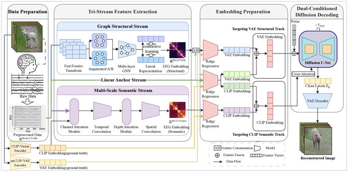
Figure 1: Schematic of TDE-Net. The diagram shows the raw EEG anchor, the sample-specific functional graph stream, the semantic temporal stream, dual-space mapping to VAE and CLIP, weighted fusion, and dual-conditioned Stable UnCLIP decoding. Tensor dimensions are indicated where applicable. Please click here to view a larger version of this figure.
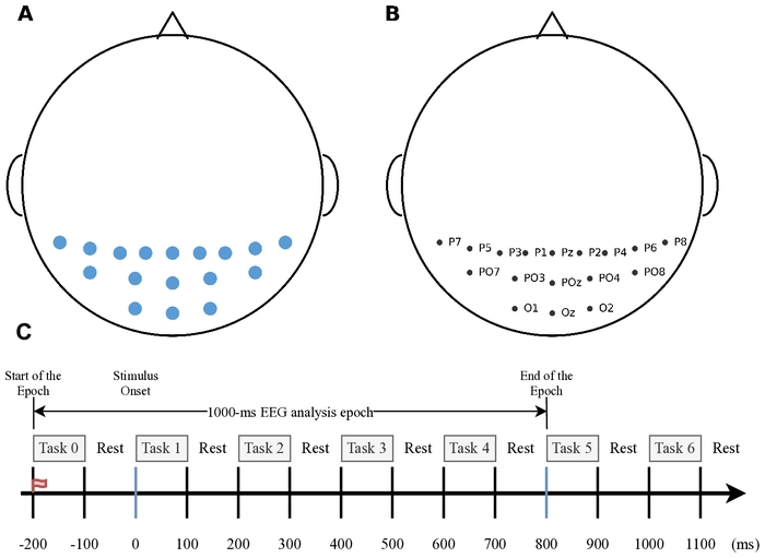
Figure 2: EEG electrode selection and experimental timing. (A) Spatial distribution of the selected 17 parieto-occipital electrodes from the original 64-channel acquisition. (B) Electrode labels: Pz, P3, P7, O1, Oz, O2, P4, P8, P1, P5, PO7, PO3, POz, PO4, PO8, P6, and P2. (C) Schematic of the RSVP timing and EEG epoch definition. In the schematic, “Task” denotes an image-presentation interval, whereas “Rest” denotes the inter-image interval; the numbered Task blocks indicate successive presentation intervals rather than different experimental conditions. Each image was presented for 100 ms with a 200-ms stimulus-onset asynchrony. The EEG epoch extended from -200 to 800 ms relative to stimulus onset, corresponding to a 1000-ms EEG analysis epoch. Please click here to view a larger version of this figure.
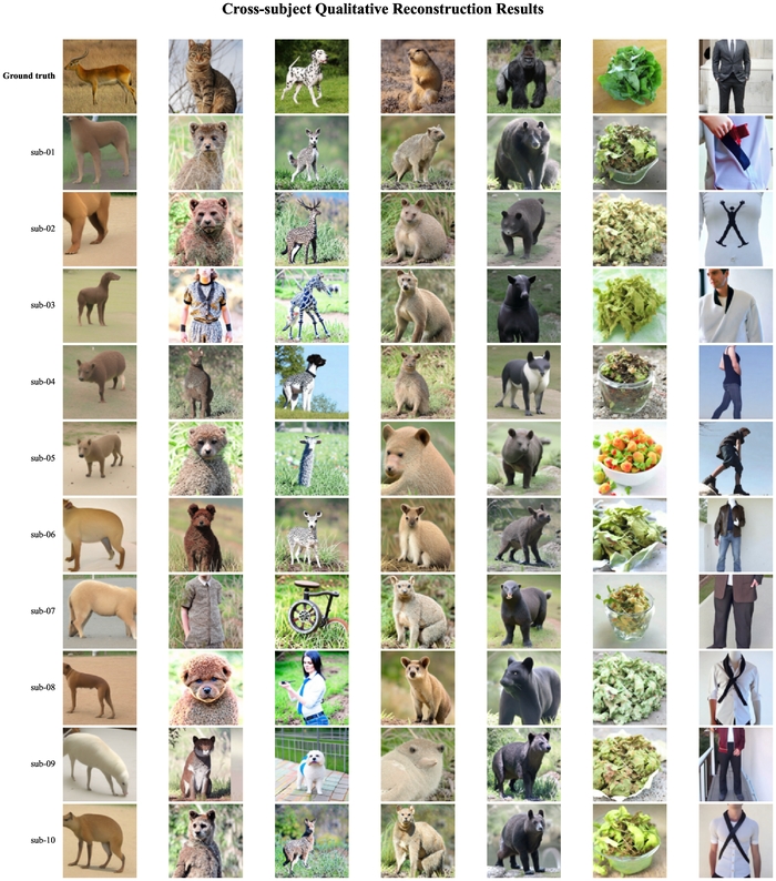
Figure 3: Cross-subject qualitative reconstruction results for seven held-out image conditions. The same zero-based condition indices (1, 32, 62, 86, 87, 108, and 175) are used for sub-01 through sub-10. The top row shows the corresponding ground-truth image samples from the THINGS-EEG2 test set, whose images were drawn from the THINGS image database34, whereas the remaining rows show TDE-Net reconstructions for each subject. The figure illustrates common semantic content and subject-level variation; quantitative cross-subject results are reported in Table 3. Please click here to view a larger version of this figure.
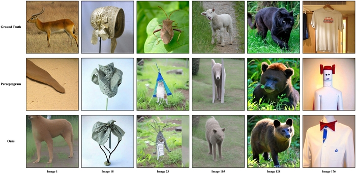
Figure 4: Qualitative reconstruction comparison for six specified sub-01 test conditions. Rows show the ground-truth stimulus, a comparator reconstruction generated by the local implementation, and the TDE-Net reconstruction; columns correspond to individual condition indices. Ground-truth image samples were drawn from the THINGS image database34. Please click here to view a larger version of this figure.
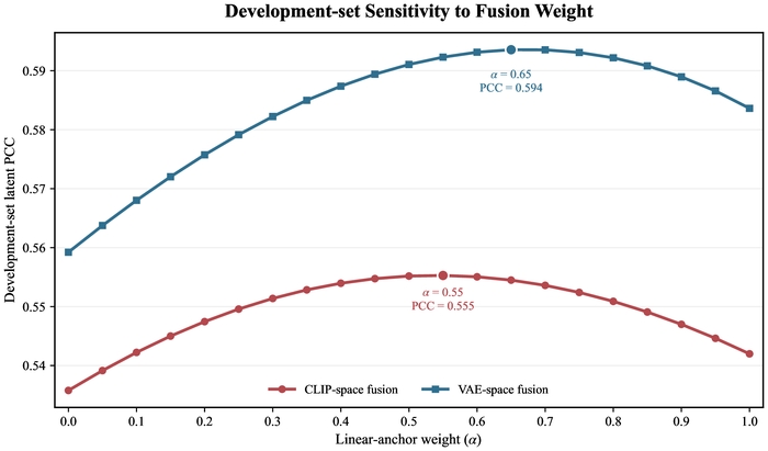
Figure 5: Development-set sensitivity of latent-fusion weights. The horizontal axis denotes the linear-anchor weight α, the complementary stream weight is 1 - α, and the vertical axis denotes development-set latent PCC. Candidate values range from 0.00 to 1.00 in increments of 0.05. CLIP- and VAE-space weights are selected independently by the maximum equally weighted mean subject-level PCC across 10 subjects, yielding αCLIP = 0.55 and αVAE = 0.65. PCC, Pearson correlation coefficient. Please click here to view a larger version of this figure.
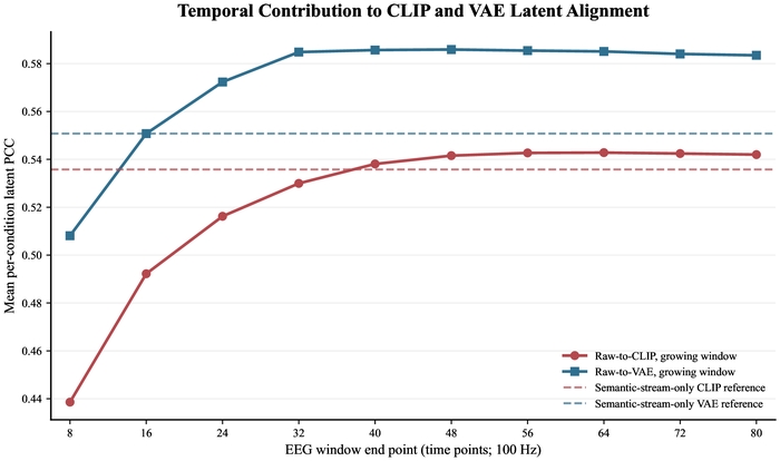
Figure 6: Temporal-window analysis of latent alignment in sub-01 (n = 200 held-out conditions). Solid curves show mean sample-wise PCC for raw-to-CLIP and raw-to-VAE ridge predictions as the EEG window endpoint expands from 8 to 80 time points at 100 Hz. Dashed lines indicate full-window semantic-stream-only CLIP and VAE reference values. PCC, Pearson correlation coefficient. Please click here to view a larger version of this figure.
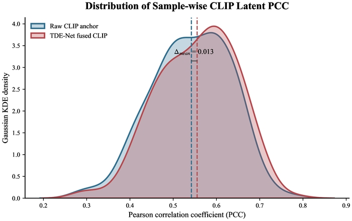
Figure 7: Distribution of sample-wise CLIP latent alignment in sub-01 (n = 200 held-out conditions). Curves are Gaussian kernel density estimates with Scott's bandwidth for the raw CLIP anchor and the frozen TDE-Net-fused CLIP prediction. Vertical dashed lines denote sample means, and the annotation indicates their difference. PCC, Pearson correlation coefficient; KDE, kernel density estimate. Please click here to view a larger version of this figure.
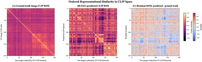
Figure 8: Ordered representational similarity in CLIP space for sub-01 (n = 200 held-out conditions). (A) Cosine-similarity RSM of L2-normalized ground-truth image CLIP embeddings. (B) Cosine-similarity RSM of fused EEG-predicted CLIP embeddings, displayed using the same ordering and color scale as panel A. (C) Residual RSM, calculated as predicted minus ground truth, displayed on a symmetric scale defined by the maximum absolute residual. Ordering is obtained by Euclidean distance and Ward linkage of ground-truth CLIP embeddings. RSM, representational similarity matrix. Please click here to view a larger version of this figure.
| Component | Parameter | Setting |
| Data and preprocessing | Dataset partition | 16,540 training and 200 held-out test conditions; 90%/10% fitting/development split (seed 42) |
| EEG input | 17 parieto-occipital channels; 0-800 ms; 100 Hz; 80 time points | |
| Spectral representation | 80-point FFT; 40 positive-frequency bins; 0-50 Hz log-amplitude spectrum | |
| Structural stream | Graph construction | Sample-specific absolute Pearson correlation; weighted top-k = 4 neighbors per node; symmetrization and self-loops |
| GCN architecture | 5 layers; 80 hidden units; ReLU; dropout 0.3; symmetric degree normalization; mean pooling | |
| Contrastive objective | 80-dimensional projection head; InfoNCE temperature τ = 0.5 | |
| Training | Adam; learning rate 5 × 10⁻⁴; batch size 32; 20 epochs; cosine annealing; minimum learning rate 10⁻⁶; seed 42 | |
| Semantic stream | Architecture | Temporal kernels 5/15/31; depth 9; 24 feature channels; dropout 0.5; output dimension 1,024 |
| Training | AdamW; learning rate 5 × 10⁻⁴; weight decay 0.01; batch size 64; 50 epochs; cosine annealing; minimum learning rate 10⁻⁶; seed 42 | |
| Latent mapping | Ridge regression | Intercept fitted; maximum iterations 50,000; inputs standardized using fitting-partition statistics |
| Regularization | CLIP penalty λ = 1,000; raw VAE penalty λ = 0; structural VAE penalty λ = 1,000 | |
| Target dimensions | CLIP: 1,024; VAE: 36,864 | |
| Fusion and decoding | Fusion weights | CLIP anchor weight α = 0.55; VAE anchor weight α = 0.65; selected on development data and fixed before testing |
| Diffusion model | sd2-community/stable-diffusion-2-1-unclip; structural scale γ = 0.02; diffusion timesteps T = 1,000 | |
| Sampling | 20 denoising steps; guidance scale 7.5; diffusion seed 0 |
Table 1: Consolidated parameter summary for TDE-Net. The table lists the data partition, preprocessing, functional adjacency construction, graph and semantic encoder settings, latent-mapping penalties, fusion weights, and diffusion-decoding settings used throughout the reported experiments.
| Method | PixCorr | SSIM | AlexNet(2) | AlexNet(5) | Inception | CLIP | EffNet | SwAV |
| Baseline | 0.141 | 0.321 | 0.823 | 0.878 | 0.704 | 0.739 | 0.898 | 0.564 |
| EEGImageDecode | - | 0.345 | 0.776 | 0.866 | 0.734 | 0.786 | - | 0.582 |
| Perceptogram (unCLIP) | 0.223 | 0.370 | 0.875 | 0.915 | 0.749 | 0.806 | 0.870 | 0.530 |
| TDE-Net (Ours) | 0.253 ± 0.014 | 0.339 ± 0.003 | 0.878 ± 0.012 | 0.915 ± 0.012 | 0.761 ± 0.021 | 0.814 ± 0.007 | 0.829 ± 0.012 | 0.509 ± 0.010 |
Table 2: Quantitative reconstruction results. The comparison methods, internal convolutional-attention Baseline, and TDE-Net were evaluated within a common experimental framework using the same THINGS-EEG2 partition, 17-channel input, preprocessing, held-out test conditions, and metric definitions, while retaining method-specific architectures. The present model is summarized as mean ± SD across 10 subjects. PixCorr, SSIM, AlexNet Layer 2, AlexNet Layer 5, Inception-v3, and CLIP are higher-is-better measures; EffNet and SwAV are correlation distances, for which lower is better. The CLIP column reports pairwise identification accuracy using the OpenAI CLIP ViT-L/14 model.
| Subject | PixCorr | SSIM | AlexNet L2 | AlexNet L5 | Inception | CLIP | EffNet | SwAV |
| sub-01 | 0.2260 | 0.3361 | 0.8831 | 0.9203 | 0.7533 | 0.8120 | 0.8567 | 0.5285 |
| sub-02 | 0.2488 | 0.3378 | 0.8699 | 0.9053 | 0.7268 | 0.8074 | 0.8335 | 0.5167 |
| sub-03 | 0.2564 | 0.3397 | 0.8728 | 0.9070 | 0.7658 | 0.8143 | 0.8268 | 0.5096 |
| sub-04 | 0.2420 | 0.3356 | 0.8598 | 0.9034 | 0.7854 | 0.8112 | 0.8255 | 0.5091 |
| sub-05 | 0.2499 | 0.3385 | 0.8760 | 0.8963 | 0.7251 | 0.8016 | 0.8394 | 0.5189 |
| sub-06 | 0.2621 | 0.3395 | 0.8910 | 0.9331 | 0.7818 | 0.8215 | 0.8202 | 0.5009 |
| sub-07 | 0.2489 | 0.3378 | 0.8643 | 0.9185 | 0.7704 | 0.8200 | 0.8222 | 0.5017 |
| sub-08 | 0.2786 | 0.3425 | 0.8951 | 0.9216 | 0.7524 | 0.8245 | 0.8214 | 0.5010 |
| sub-09 | 0.2609 | 0.3370 | 0.8775 | 0.9238 | 0.7662 | 0.8055 | 0.8250 | 0.5009 |
| sub-10 | 0.2571 | 0.3433 | 0.8871 | 0.9240 | 0.7792 | 0.8175 | 0.8140 | 0.4977 |
| Mean | 0.2531 | 0.3388 | 0.8777 | 0.9153 | 0.7606 | 0.8135 | 0.8285 | 0.5085 |
| Mean ± SD | 0.2531 ± 0.0138 | 0.3388 ± 0.0025 | 0.8777 ± 0.0115 | 0.9153 ± 0.0116 | 0.7606 ± 0.0213 | 0.8135 ± 0.0074 | 0.8285 ± 0.0122 | 0.5085 ± 0.0101 |
| 95% CI | 0.2432-0.2630 | 0.3370-0.3406 | 0.8695-0.8859 | 0.9070-0.9236 | 0.7454-0.7759 | 0.8082-0.8189 | 0.8198-0.8372 | 0.5013-0.5157 |
Table 3: Cross-subject quantitative results for TDE-Net. Each subject contributes 200 held-out test conditions. The table reports the eight metrics for sub-01 through sub-10, followed by the across-subject mean, sample SD, and 95% CI. CLIP denotes OpenAI CLIP ViT-L/14 pairwise identification accuracy; EffNet and SwAV are lower-is-better correlation distances.
| Method | PixCorr | SSIM | AlexNet(2) | AlexNet(5) | Inception | CLIP | EffNet | SwAV |
| Linear Anchor | 0.2157 | 0.3309 | 0.8891 | 0.9128 | 0.7493 | 0.7967 | 0.8683 | 0.5394 |
| Linear + Struct-Stream | 0.2318 | 0.3393 | 0.8861 | 0.9319 | 0.7439 | 0.7996 | 0.8657 | 0.5359 |
| Linear + Sem-Stream | 0.2372 | 0.3382 | 0.8879 | 0.9228 | 0.7447 | 0.8026 | 0.8655 | 0.5307 |
| TDE-Net (Ours) | 0.2531 | 0.3388 | 0.8777 | 0.9153 | 0.7607 | 0.8135 | 0.8285 | 0.5085 |
Table 4: Ablation results reported as across-subject mean values under the evaluation procedure described in Protocol Section 6. The Linear Anchor is a locally evaluated internal direct ridge-mapping reference; the structural, semantic, and complete configurations use the same condition indices and metric definitions. PixCorr, SSIM, AlexNet Layer 2, AlexNet Layer 5, Inception-v3, and CLIP are higher-is-better measures; EffNet and SwAV are lower-is-better correlation distances. Values are shown to three decimal places.
Supplementary Figure 1: Representative reconstruction cases spanning the CLIP-agreement range for sub-01. The 200 held-out conditions are ranked by cosine similarity between fused EEG-predicted and ground-truth CLIP embeddings; six best, six median, and six worst cases are shown. Each column pairs a ground-truth image sample from the THINGS-EEG2 test set with its TDE-Net reconstruction. The ground-truth images were drawn from the THINGS image database34. Please click here to download this file.
Supplementary Figure 2: Joint visualization of ground-truth and EEG-predicted CLIP representations in sub-01 (n = 200 conditions per representation). (A) Ground-truth CLIP representations. (B) EEG-predicted CLIP representations. Colors denote five k-means clusters fitted to L2-normalized ground-truth CLIP embeddings (k = 5, n_init = 50, seed = 7). The clusters are data-driven groups and do not correspond to predefined semantic categories. Ground-truth and predicted embeddings are concatenated, reduced to 50 dimensions by PCA, and jointly projected by t-SNE (perplexity = 28, learning rate = auto, Euclidean metric, seed = 12). PCA, principal component analysis; t-SNE, t-distributed stochastic neighbor embedding. Please click here to download this file.
Supplementary Figure 3: EEG patterns grouped by broad image-concept category for sub-01. Concepts are assigned to Animals, Food/plant-related concepts, or Other objects. Within each category, rows follow Ward's hierarchical ordering of whitened ground-truth CLIP embeddings and are uniformly sampled to at most 30 concepts for legibility. The columns show 17 EEG channels, with 80 time points per channel. The color scale (-1 to 1) represents clipped, normalized whitened EEG amplitude. Please click here to download this file.
Supplementary Figure 4: Semantic-stream scalp-channel attention topography. Colors show normalized relative magnitudes of learned channel-weight parameters across the selected 17 electrodes in a standard 10–20 scalp projection; electrode dots and labels identify measurement positions. The scale ranges from 0 to 1 and summarizes the model's learned relative channel weighting. Please click here to download this file.
토론
본 연구는 EEG 전처리, 구조적 및 의미적 표현 학습, CLIP/VAE 잠재 매핑, 융합 및 확산 디코딩을 분리한 모듈형 계산 워크플로우를 제시합니다. 이러한 단계적 구성은 중간 출력물을 생성된 이미지와 별개로 검토할 수 있게 하며, 소형 EEG 인코더에서 교차 모달 및 확산 기반 재구성 방법으로 이어지는 광범위한 발전 과정을 따릅니다6,11,12,13,14,15,16,,17,18,19,20,21,22. 피험자 간 분석에서는 10명의 피험자를 대상으로 한 홀드아웃 평가에 대해 피험자별 수치와 피험자 전체 평균 및 표본 표준편차(SD)를 보고합니다. 표 4의 단계별 어블레이션 분석과 함께, 본 분석은 보고된 파이프라인 내에서 스트림별 효과와 피험자 간 변동성을 정량화합니다.
핵심 단계 및 문제 해결
가장 중요한 구현 제어 요소는 파티션 격리, 일관된 정규화, 조건-인덱스 보존 및 분리된 CLIP/VAE 매핑입니다. 퓨전 가중치는 개발 조건에서 선택되어야 하며, 테스트 재구성을 수행하기 전에 동결되어야 합니다. 성능이 예상보다 낮을 경우, 먼저 배열 순서와 차원을 확인한 다음, 원시 및 분기별 잠재 PCC, 퓨전 메타데이터, 이미지 레벨 메트릭 출력을 검사하십시오. 잠재 정렬 실패는 상위 매핑 문제를 나타내며, 잠재 변수는 안정적이지만 이미지가 가변적인 경우는 확률적 또는 디코더 의존적 동작을 반영할 수 있습니다14,21,22,29.
전극 몽타주, 샘플링 속도 또는 시간 창을 변경하려면 그래프 구성, 스펙트럼 특성 및 시간 커널에 상응하는 변경이 필요합니다. 단일 점수만으로는 픽셀 충실도, 구조 및 객체 수준의 일치도를 모두 포착할 수 없으므로, 보완적인 저수준 및 세만틱 척도를 통해 재구성 품질을 평가해야 합니다6,11,21,22,23. 여기서 사용된 CLIP 척도는 쌍별 식별 정확도인 반면, 그림 7 및 그림 8에서는 잠재 수준 PCC를 사용하며, 이 두 값은 서로 대체될 수 없습니다.
TDE-Net의 모듈식 구조는 상보적인 EEG 표현이 시각적 재구성의 구조적 및 의미적 측면에 서로 다르게 기여하는지 조사할 수 있는 프레임워크를 제공합니다. 이러한 접근 방식은 최종 재구성된 이미지에만 의존하지 않고 EEG 특징 표현, 잠재 타겟 및 생성 디코더를 체계적으로 비교하는 것을 용이하게 할 수 있습니다. 대안적인 접근 방식으로는 직접적인 선형 EEG-to-latent 매핑, 단일 스트림 컨볼루션 또는 어텐션 기반 인코더, 그래프 기반 표현 및 엔드-투-엔드 신경 디코딩 프레임워크가 있습니다6,7,8,9,10,11,17,18,19,20,21,22. 본 워크플로우는 시각적 지각 디코딩, 신경 표현 분석 및 비침습적 뇌-컴퓨터 인터페이스 연구에 특히 유용할 수 있으며, 여기서 중간 단계의 EEG-to-latent 예측을 분리함으로써 어떤 구성 요소가 재구성 성능에 기여하는지 특성화하는 데 도움이 될 수 있습니다.
한계점
주요 한계점은 고정된 THINGS-EEG2 RSVP 획득 방식, 선택된 17개의 두정-후두 채널, 피험자별 매핑, 단일 확산 디코더 및 정성적 해석 분석입니다21,22,23. 10명의 피험자 요약은 데이터셋 내 피험자 간 변동성을 다루고 있지만, 데이터셋 간 또는 패러다임 간 전이를 입증하지는 않습니다. 생성된 이미지는 EEG 입력으로 뒷받침되지 않는 그럴듯한 세부 사항을 포함할 수 있으며, RSM, t-SNE, EEG 패턴 및 어텐션 뷰는 인과적인 신경 메커니즘을 입증하지 않습니다. 단계별 어블레이션은 공유된 raw EEG 앵커, 잠재 타겟, 확산 디코더 및 평가 프로토콜 하에서 구조적 스트림, 의미적 스트림 및 듀얼 스페이스 퓨전의 기여도를 특성화합니다.
향후 연구 방향
이러한 제약 조건 내에서, 본 결과는 확산 디코딩(diffusion decoding) 이전에 별도의 시맨틱 및 이미지 잠재 공간에서 상보적인 EEG 표현을 평가하는 것을 뒷받침합니다. 향후 연구에서는 독립적인 데이터셋, 피험자 적응, 불확실성 추정, 대안적인 채널 몽타주, 그리고 지원되지 않는 시각적 세부 사항에 대해 더 강력한 제어를 갖춘 디코더를 테스트해야 합니다14,15,16,17,18,19,20,21,22,23. 현재의 발견을 더 광범위한 신경과학 또는 뇌-컴퓨터 인터페이스 환경으로 확장하기 전에 이러한 연구들이 필요합니다.
결론:
TDE-Net은 가공되지 않은 EEG 앵커를 구조적 및 의미적 EEG 표현과 결합하고, 이를 VAE 및 CLIP 잠재 공간과 각각 정렬시킨 후, 확산 디코딩 이전에 결과 예측값들을 통합합니다. 10명의 THINGS-EEG2 참가자를 대상으로 한 실험에서, 재구성된 이미지는 시각 자극과 픽셀 수준, 구조적 및 의미적 대응 관계가 측정 가능한 수준으로 유지되었으며, 단계별 제거 분석(ablation)을 통해 구조적 스트림, 의미적 스트림 및 이중 공간 융합의 효과를 구분하였습니다. 중간 EEG 특징, 잠재 예측값, 융합 출력물 및 최종 재구성 결과를 공개함으로써, 본 프로토콜은 EEG 기반 시각 재구성을 연구하고 이를 독립적인 데이터 세트 및 획득 환경으로 향후 확장하여 평가하기 위한 재현 가능한 프레임워크를 제공합니다.
공개 사항
저자들은 본 연구에 영향을 미칠 수 있는 경쟁적인 재정적 이해관계나 개인적 관계가 없음을 밝힙니다. 저자들은 원고 작성, 코드, 데이터 분석 또는 그림 준비 과정에서 생성형 AI 도구를 사용하지 않았음을 밝힙니다.
감사의 글
본 연구는 중국 국가자연과학재단 (Grant No. 62433002 및 Grant No. 62476014), 국가과학기술 중점 프로젝트 (No. 2021ZD0113703), 베이징시 사회과학기금 연차 계획 프로젝트 (No. 23GLB014), 베이징시 기관 고수준 혁신 팀 구축 및 지원 프로젝트 (Grant No. BPHR20220104) 및 베이징 학자 프로그램 (Grant No. 099)의 지원을 받아 수행되었습니다.
재료
| 이름 | 회사 | 카탈로그 번호 | 댓글 |
|---|---|---|---|
| 가속화 | Hugging Face | 0.30.1 | 디퓨전 파이프라인 장치 관리; https://github.com/huggingface/accelerate |
| CLIP ViT-L/14 | OpenAI | ViT-L/14; openai-clip 1.0.1 | 시맨틱 타겟 및 CLIP 쌍별 식별에 사용된 이미지 특징 인코더; https://github.com/openai/CLIP |
| 디퓨저 | Hugging Face | 0.32.2 | Stable UnCLIP 파이프라인 구현; https://github.com/huggingface/diffusers |
| Matplotlib | Matplotlib 개발팀 | 3.10.6 | 과학적 도표 생성; https://matplotlib.org/ |
| MNE-Python | MNE 개발자들 | 1.11.0 | 표준 10-20 전극 배치법 및 두피 채널 토포그래피; https://mne.tools/ |
| NumPy | NumPy 개발자 | 2.3.4 | EEG 어레이, 잠재 임베딩, 융합 및 메트릭 집계; https://numpy.org/ |
| NVIDIA GeForce RTX 4070 노트북 GPU | NVIDIA | 8 GB; 드라이버 595.97 | 로컬 인코더 학습 및 확산 재구성에 사용된 GPU. |
| 필로우(Pillow) | Python Imaging Library 포크 | 11.1.0 | 이미지 로딩, 크기 조정 및 내보내기; https://python-pillow.org/ |
| 파이썬 | Python Software Foundation | 3.12.12 | 주 실행 환경; https://www.python.org/ |
| PyTorch | PyTorch Foundation | 2.9.1+cu128 | EEG 인코더 학습 및 신경망 추론; https://pytorch.org/ |
| scikit-image | scikit-image 개발자 | 0.25.2 | SSIM 및 이미지 처리 유틸리티; https://scikit-image.org/ |
| scikit-learn | scikit-learn 개발자 | 1.7.2 | 능선 회귀, k-평균 군집화, 주성분 분석, t-SNE; https://scikit-learn.org/ |
| SciPy | SciPy 개발자 | 1.16.3 | 상관관계, 통계적 거리 및 계층적 군집 분석; https://scipy.org/ |
| Seaborn | Seaborn 개발자 | 0.13.2 | 가우시안 커널 밀도 시각화; https://seaborn.pydata.org/ |
| 시맨틱 스트림 EEG 인코더 | TDE-Net 저자; LMDA-Net에서 수정됨 | 저장소 커밋 c99325d | 다중 스케일 시간적 의미 표현; 구현 및 체크포인트 메타데이터는 코드 저장소에 제공됩니다. |
| Stable Diffusion 2.1 UnCLIP | Stability AI / SD2 커뮤니티 | sd2-community/stable-diffusion-2-1-unclip | 동결 확산 디코더; https://huggingface.co/sd2-community/stable-diffusion-2-1-unclip |
| 구조적 스트림 EEG 인코더 | TDE-Net 저자들 | 리포지토리 커밋 c99325d | 자기 지도 학습 기반 그래프 표현; 원시 EEG 및 그래프 특징은 VAE 공간의 구조적 매핑을 위해서만 결합됩니다. |
| TDE-Net 정렬, 융합, 평가 및 시각화 스크립트 | Yuan-ui198 | 커밋 c99325d7f9e090ddd7cd581 제공된 텍스트가 없습니다. 번역할 내용을 입력해 주세요. | 제공해주신 링크는 GitHub 저장소(TDE-Net)의 특정 커밋 버전입니다. 해당 저장소의 내용(코드, README 파일 등)을 바탕으로 번역이 필요하신 구체적인 텍스트를 제공해 주시면, 요청하신 전문 학술 번역 지침에 따라 정확하게 한국어로 번역해 드리겠습니다. 제공된 텍스트가 없습니다. 번역할 소스 텍스트를 입력해 주세요. |
| THINGS 데이터베이스 | Hebart 등 | doi:10.1371/journal.pone.0223792 | 자연주의적 객체 자극 소스; https://things-initiative.org/ |
| THINGS-EEG2 데이터셋 | Gifford 등 | doi:10.1016/j.neuroimage.2022.119754 | 피험자 10명의 64채널 EEG; 본 연구에서는 17개의 두정-후두 채널을 선택함; https://osf.io/anp5v/ |
| timm | Ross Wightman 및 기여자들 | 1.0.22 | 특징 평가에 사용되는 사전 훈련된 비전 모델 유틸리티; https://github.com/huggingface/pytorch-image-models |
| torchvision | PyTorch Foundation | 0.24.1+cu128 | AlexNet, Inception-v3 및 EfficientNet 평가 백본; https://pytorch.org/vision/ |
| tqdm | tqdm 개발자 | 4.67.1 | 특징 추출, 재구성 및 평가를 위한 진행 상황 보고; https://tqdm.github.io/ |
| 트랜스포머 | Hugging Face | 4.37.2 | 사전 학습된 모델 구성 요소에 대한 인터페이스; https://github.com/huggingface/transformers |
참고문헌
- Shen G, Horikawa T, Majima K, Kamitani Y. Deep image reconstruction from human brain activity. PLoS Comput Biol. 2019;15(1):e1006633. doi:10.1371/journal.pcbi.1006633.
- Chen Z, Qing J, Xiang T, Yue W, Zhou JH. Seeing beyond the brain: conditional diffusion model with sparse masked modeling for vision decoding. In: Proceedings of the IEEE/CVF Conference on Computer Vision and Pattern Recognition. 2023. p. 22710-22720. Available from: https://openaccess.thecvf.com/content/CVPR2023/html/Chen_Seeing_Beyond_the_Brain_Conditional_Diffusion_Model_With
_Sparse_Masked_Modeling_CVPR_2023_paper.html - Takagi Y, Nishimoto S. High-resolution image reconstruction with latent diffusion models from human brain activity. In: Proceedings of the IEEE/CVF Conference on Computer Vision and Pattern Recognition. 2023. p. 14453-14463. Available from: https://openaccess.thecvf.com/content/CVPR2023/html/Takagi_High-Resolution_Image_Reconstruction_With_Latent_Diffusion_Models_
From_Human_Brain_CVPR_2023_paper.html - Scotti PS et al. Reconstructing the mind's eye: fMRI-to-image with contrastive learning and diffusion priors. Adv Neural Inf Process Syst. 2023;36:24705-24728. doi:10.52202/075280-1073.
- Geman S, Bienenstock E, Doursat R. Neural networks and the bias/variance dilemma. Neural Comput. 1992;4(1):1-58. doi:10.1162/neco.1992.4.1.1.
- Lawhern VJ et al. EEGNet: a compact convolutional neural network for EEG-based brain-computer interfaces. J Neural Eng. 2018;15(5):056013. doi:10.1088/1741-2552/aace8c.
- Kostas D, Aroca-Ouellette S, Rudzicz F. BENDR: using transformers and a contrastive self-supervised learning task to learn from massive amounts of EEG data. Front Hum Neurosci. 2021;15:653659. doi:10.3389/fnhum.2021.653659.
- Song Y, Zheng Q, Liu B, Gao X. EEG Conformer: convolutional transformer for EEG decoding and visualization. IEEE Trans Neural Syst Rehabil Eng. 2023;31:710-719. doi:10.1109/TNSRE.2022.3230250.
- Cui CM et al. "Pre-Train, Prompt" framework to boost graph neural networks performance in EEG analysis. IEEE J Biomed Health Inform. 2025;29(7):4847-4860. doi:10.1109/JBHI.2025.3541058.
- Meng X, Qiu S, Wan S, Cheng K, Cui L. A motor imagery EEG signal classification algorithm based on recurrence plot convolution neural network. Pattern Recognit Lett. 2021;146:134-141. doi:10.1016/j.patrec.2021.03.023.
- Miao Z, Zhao M, Zhang X, Ming D. LMDA-Net: a lightweight multi-dimensional attention network for general EEG-based brain-computer interfaces. Neuroimage. 2023;276:120209. doi:10.1016/j.neuroimage.2023.120209.
- Zhang S, Tang C, Guan C. Visual-to-EEG cross-modal knowledge distillation for continuous emotion recognition. Pattern Recognit. 2022;130:108833. doi:10.1016/j.patcog.2022.108833.
- Palazzo S et al. Decoding brain representations by multimodal learning of neural activity and visual features. IEEE Trans Pattern Anal Mach Intell. 2021;43(11):3833-3849. doi:10.1109/TPAMI.2020.2995909.
- Rombach R, Blattmann A, Lorenz D, Esser P, Ommer B. High-resolution image synthesis with latent diffusion models. In: Proceedings of the IEEE/CVF Conference on Computer Vision and Pattern Recognition. 2022. p. 10684-10695. Available from: https://openaccess.thecvf.com/content/CVPR2022/html/Rombach_High-Resolution_Image_Synthesis_With_Latent_Diffusion_Models_CVPR
_2022_paper.html - Radford A et al. Learning transferable visual models from natural language supervision. In: Proceedings of the 38th International Conference on Machine Learning. PMLR. 2021;139:8748-8763. Available from: https://proceedings.mlr.press/v139/radford21a.html
- Bai Y et al. DreamDiffusion: high-quality EEG-to-image generation with temporal masked signal modeling and CLIP alignment. In: Computer Vision - ECCV 2024. Cham: Springer; 2024. p. 472-488. doi:10.1007/978-3-031-72751-1_27.
- Cao X, Gong P, Zhang L, Zhang D. EEG-CLIP: a transformer-based framework for EEG-guided image generation. Neural Netw. 2026;194:108167. doi:10.1016/j.neunet.2025.108167.
- Liu Y et al. FSDBN: foreground-aware EEG-visual alignment via dynamic brain networks. arXiv [Preprint]. 2026. Available from: https://arxiv.org/abs/2607.18344
- Yin F, Zheng C, Gong P, Guan D, Zhu Q. Neural visual decoding via cognitive-guided adaptive blurring and information-constrained alignment. arXiv [Preprint]. 2026. Available from: https://arxiv.org/abs/2605.16418
- Liu J, Gong P, Zheng C, Liu Y, Zhu Q. Multi-level bidirectional biomimetic learning for EEG-based visual decoding. arXiv [Preprint]. 2026. Available from: https://arxiv.org/abs/2605.04680
- Fei T et al. Perceptogram: reconstructing visual percepts and presumptive electrode preference from EEG. arXiv [Preprint]. 2024. Available from: https://arxiv.org/abs/2404.01250
- Li D, Wei C, Li S, Zou J, Liu Q. Visual decoding and reconstruction via EEG embeddings with guided diffusion. Adv Neural Inf Process Syst. 2024;37:102822-102864. doi:10.52202/079017-3266.
- Gifford AT, Dwivedi K, Roig G, Cichy RM. A large and rich EEG dataset for modeling human visual object recognition. Neuroimage. 2022;264:119754. doi:10.1016/j.neuroimage.2022.119754.
- Kipf TN, Welling M. Semi-supervised classification with graph convolutional networks. In: International Conference on Learning Representations. 2017. Available from: https://openreview.net/forum?id=SJU4ayYgl
- Chen T, Kornblith S, Norouzi M, Hinton G. A simple framework for contrastive learning of visual representations. In: Proceedings of the 37th International Conference on Machine Learning. PMLR. 2020;119:1597-1607. Available from: https://proceedings.mlr.press/v119/chen20j.html
- Ramoser H, Muller-Gerking J, Pfurtscheller G. Optimal spatial filtering of single trial EEG during imagined hand movement. IEEE Trans Rehabil Eng. 2000;8(4):441-446. doi:10.1109/86.895946.
- Bai S, Kolter JZ, Koltun V. An empirical evaluation of generic convolutional and recurrent networks for sequence modeling. arXiv [Preprint]. 2018. Available from: https://arxiv.org/abs/1803.01271
- Woo S, Park J, Lee JY, Kweon IS. CBAM: convolutional block attention module. In: European
Conference on Computer Vision. Cham: Springer; 2018. p. 3-19. Available from:
https://doi.org/10.1007/978-3-030-01234-2_1 - Hoerl AE, Kennard RW. Ridge regression: biased estimation for nonorthogonal problems. Technometrics. 1970;12(1):55-67. doi:10.1080/00401706.1970.10488634.
- Zhou ZH. Ensemble Methods: Foundations and Algorithms. Boca Raton: Chapman and Hall/CRC; 2012.
- Ho J, Jain A, Abbeel P. Denoising diffusion probabilistic models. Adv Neural Inf Process Syst. 2020;33:6840-6851. Available from: https://proceedings.neurips.cc/paper/2020/hash/4c5bcfec8584af0d967f1ab10179ca4b-Abstract.html
- Ho J, Salimans T. Classifier-free diffusion guidance. arXiv [Preprint]. 2022. Available from: https://arxiv.org/abs/2207.12598
- Kingma DP, Welling M. Auto-encoding variational Bayes. In: International Conference on Learning Representations. 2014. Available from: https://openreview.net/forum?id=33X9fd2-9FyZd
- Hebart MN et al. THINGS: a database of 1,854 object concepts and more than 26,000 naturalistic object images. PLoS One. 2019;14(10):e0223792. doi:10.1371/journal.pone.0223792.
재인쇄 및 허가
이 논문이 게재되었습니다
동영상 곧 제공