Evaluation of Ribbon Synapses at Specific Frequency Regions of Mouse Cochlea

Abstract

Source: Yu, S., et al. Morphological and Functional Evaluation of Ribbon Synapses at Specific Frequency Regions of the Mouse Cochlea. J. Vis. Exp. (2019).

This video demonstrates a method for evaluating ribbon synapses in specific regions of the mouse cochlea. It utilizes immunostaining and confocal imaging techniques to identify functional synapses across different frequency regions in each cochlear turn.

Protocol

All procedures involving animal handling have been performed in accordance with the institute's IRB guidelines.

1. Animal Selection

1. For all experiments, use adult C57BL/6J male mice (8 weeks old) as the animal model.
   NOTE: C57BL/6J mice carrying a splice variant of the Cdh23 exhibit accelerated senescence in the auditory system, reflected as a 40% loss of ribbon synapses at the basal turn of the cochlea and a 10% loss at the middle turn by 6 months of age, followed by a rapid increase of this loss in the whole cochlea with age. Thus, we advise caution when using C57BL/6J mice older than 6 months for auditory research. Other strains of mice can be used depending on specific experimental aims.
2. Inspect the mice using a professional diagnostic pocket otoscope to rule out outer or middle ear pathologies prior to hearing assessments. Potential signs may include fluid or pus in the external auditory canal, redness and swelling in local tissue, and tympanic membrane perforation.
   NOTE: Although this is rarely encountered, once identified, mice with outer or middle ear diseases should be excluded.

2. Hearing Assessment

1. Anesthetize mice using an intraperitoneal injection of a mixture of ketamine hydrochloride (100 mg/kg) and xylazine hydrochloride (10 mg/kg). Judge the depth of anesthesia via painful stimuli (e.g., toe-pinch reflex).
   NOTE: When the toe-pinch reflex is completely absent, the animal has reached an adequate depth of anesthesia for auditory testing. If more time is required for bilateral ABR (auditory brainstem response) recordings, administer a lower dosage (one-fifth the original dosage) of anesthetics to restore the original anesthetic plane. Take care to avoid anesthetic overdose, as this may lead to death in mice.
2. Maintain the anesthetized animal's body temperature at 37.5 °C using a thermoregulating heating pad. Place the anesthetized animal in an electrically and acoustically shielded room to avoid interference throughout the hearing test.
   NOTE: Maintain the physiological temperature during the entire procedure until the animal is totally awake in order to prevent death caused by post-anesthesia hypothermia.
3. Place subdermal needle electrodes (20 mm, 28 G) at the vertex of the skull (recording electrode), in the ipsilateral parotid region below the pinna of the measured ear (reference electrode), and in the contralateral parotid region (ground electrode), with a depth of 3 mm under the skin of the mouse head, respectively.
4. Use a closed-field speaker to perform acoustic stimulation via a 2 cm plastic tube with a cone-shaped tip. Fit the tip into the external ear canal.
   NOTE: Ensure that the electrical impedance in the recording and reference electrodes is less than 3 kOhm (usually 1 kOhm). If the impedance is high, change the insertion site of the electrode, clean the electrode with alcohol, or replace the electrode to avoid alterations in ABR wave amplitude.
5. For ABR recording, generate tone pips (3 ms duration, 1 ms rise/fall times, at a rate of 21.1/s, frequency: 4–48 kHz) and present them at decreasing sound pressure levels (SPLs) from 90 to 10 dB in 5‒10 dB SPL steps. During this step, the responses are amplified (10,000 times), filtered (0.1–3 kHz), and averaged (1,024 samples/stimulus level).
   NOTE: ABRs are collected for each stimulus level in 10 dB steps, with an additional 5 dB steps near the threshold.
6. At each frequency, determine the ABR threshold, which refers to the minimal SPL resulting in a reliable ABR recording with one or more distinguishable waves that can be clearly identified by visual inspection.
   NOTE: It is usually necessary to repeat the process for low SPLs around the threshold to ensure the consistency of the waveforms. The response threshold is the lowest stimulus level at which the waveform can be observed when a decrease of 5 dB would lead to the disappearance of the waveform.

3. Cochlear Tissue Processing

1. After ABR recording, euthanize the anesthetized mice via cervical dislocation, decapitate them, expose the bulla from the ventral side, and open them with sharp scissors to gain access to the cochlea.
2. Using fine forceps, remove the temporal bones, sever the stapes artery, remove the stapes from the oval window, and rupture the round window membrane. Make a small hole at the apex of the cochlea by gently rotating the tip of a needle (13 mm, 27 G).
3. Fix the isolated bones with 4% (wt/vol) paraformaldehyde in 0.1 M phosphate-buffered saline (PBS, pH 7.4) overnight at 4 °C. Using a fine-tipped pipette, gently flush fixative through the perilymphatic spaces via application to the oval or round windows (as an inlet) and the opening at the apex (as an outlet).
   NOTE: Some proteins require a short duration of fixation to avoid destruction of their epitopes for immunolabeling. In such cases, incubate bones in 4% paraformaldehyde at room temperature (RT) for 2 h, depending on the manufacturer’s instructions for immunohistochemistry. Fixation can also be performed via cardiac perfusion to remove the cochlear blood, avoiding background noise due to non-specific staining at later stages, particularly in mouse models of cochlear synaptopathy.
4. Rinse the bones three times for 5 min with 0.1 M cold PBS to remove residual paraformaldehyde. Decalcify the bones with 10% ethylenediaminetetraacetic acid (EDTA) either at RT for 4 h or at 4 °C for 24 h via gentle shaking in a horizontal shaker at 20 rpm. EDTA can be refreshed midway.
   NOTE: Decalcification times are subject to the concentration of EDTA and users’ preferences. Decalcified tissue should maintain a certain degree of toughness, which facilitates the manipulation of isolating cochlear whole mounts at later steps. Temporal bones can be decalcified in 10% EDTA with rotation, allowing researchers to leave the laboratory following ABR tests and fixation experiments. The decalcification time is flexible within the range of 20 to 30 h at 4 °C.
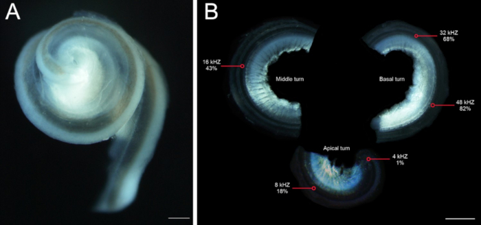
5. Transfer one decalcified temporal bone from EDTA to 0.1 M PBS. Use #3 and #5 Dumont forceps and the 27 G needle to dissect the apical, middle, and basal cochlear regions in turn and then dissect the cochlea out of the bone under a stereo dissection microscope. Make a series of small cuts along the spiral ligament using a razor blade, and remove the tectorial membrane and Reissner’s membrane (Figure 1).
   NOTE: As long as the dissected cochlea is intact, this process can be modified according to the individual operator's usual protocol.
6. Further dissect the remaining auditory epithelium including the spiral limbus into individual cochlear turns (apex, middle, and base with hook region) for whole-mount preparations.
7. Under a 40x oil objective of a light microscope, measure the basilar membrane length with a 250 μm scale placed in the eyepiece, which can be adjusted along the stereocilia of the IHCs.
8. Calculate the length of each cochlear turn by adding all segment lengths (250 μm per segment), and concomitantly obtain the total length of the basilar membrane by summing the lengths of each turn.
9. Convert the total length of the basilar membrane, including the hook region, into a percentage based on distance from the cochlear apex (0% refers to the cochlear apex, 100% to the cochlear base).
10. Convert this distance into the cochlear characteristic frequency using a logarithmic function (d(%) = 1 - 156.5 + 82.5 × log(f), with a slope of 1.25 mm/octave of frequency, where d is the normalized distance from the cochlear apex in percent, f is the frequency in kHz), as previously described. Thus frequency range in a corresponding area of the basilar membrane on each cochlear turn can be acquired.

4. Immunofluorescence Staining

1. After dissection, place each cochlear turn in a separate 2.5 mL centrifuge tube and incubate cochlear turns in 10% goat serum/PBS/0.1% Triton X-100 for 1 h at RT on a rotator.
2. Remove the above blocking/permeabilization solution from each tube using a 200 μL pipette tip under a dissection microscope and incubate the specimens with primary antibodies diluted in 5% goat serum/PBS/0.1% Triton X-100 overnight at 4 °C on a rotator.
   NOTE: For immunolabeling of cochlear synaptic ribbons, use the presynaptic marker mouse anti-carboxyl-terminal binding protein 2 IgG1 (CtBP2, labeling the B domain of the RIBEYE scaffolding protein, 1:400) and the postsynaptic marker mouse anti-glutamate receptor 2 IgG2a (GluR2, labeling a subunit of the α-amino-3-hydroxy-5-methyl-4-isoxazolepropionic acid or AMPA receptor, 1:200).
3. Rinse three times for 5 min with 0.1 M cold PBS to remove residual primary antibodies and incubate the specimens with secondary antibodies diluted in 5% goat serum/PBS/0.1% Triton X-100 at RT for 2‒3 h in darkness on a rotator.
   NOTE: Prepare appropriate secondary antibody mixtures using goat anti-mouse Alexa Fluor 568 (IgG1, 1:500) and goat anti-mouse Alexa Fluor 488 (IgG2a, 1:500), which are complementary to the primary antibodies used in step 4.2. To improve labeling efficiency for synaptic ribbons, we recommend selecting specific secondary antibodies. Some labs extend incubation with secondary antibodies to increase GluR2 immunolabeling.
4. Rinse three times for 5 min with 0.1 M PBS to remove residual secondary antibodies and transfer the specimens from 2.5 mL centrifuge tubes to 35 mm plates containing 0.1 M PBS.
5. Place a drop of mounting medium containing 4’,6-diamidino-2-phenylindole (DAPI) onto the slide and transfer the specimens from PBS to the mounting medium. Place one edge of a coverslip on the slide and release to let the coverslip fall gently.
   NOTE: To ensure that the hair cells face upward and that no folding or twisting of cochlear specimens occurs during the procedure, mount cochlear specimens under a stereo dissection microscope.
6. Place the slides in a slide box at 4 °C overnight to let slides dry and then image under a laser confocal microscope.

5. Morphological Evaluation of Cochlear Ribbon Synapses

1. Image slides using a confocal microscope with three lasers—a 405 nm UV diode, a 488 nm argon laser, and a 561 nm diode-pumped solid-state (DPSS) laser to excite DAPI (Excitation spectrum 409–464 nm), Alexa Fluor 488 (Excitation spectrum 496–549 nm) and Alexa Fluor 568 (Excitation spectrum 573–631 nm), respectively.
2. Acquire confocal z-stacks over a distance of 8 μm from each cochlear turn using a 63x high-resolution oil immersion lens.
   ​NOTE: Once defined, all parameters for digitizing photomicrographs should be saved and applied uniformly to all slides.
3. For synaptic punctum counts, set the z-stacks (0.3 μm step size) to span the entire length of inner hair cells (IHCs), thereby ensuring that all synaptic puncta can be imaged.
4. Merge the images containing puncta in a z-stack to obtain the z-axis projection, and import to the image-processing software.
5. Divide synaptic total counts in each z-stack at specific frequency regions by the number of IHCs (equal to the DAPI nuclear manual counts) to calculate the number of synaptic puncta for each IHC. At each specific frequency region, average all synaptic puncta in three images of different microscopic fields containing 9–11 IHCs.
   1. Outline the region of interests (ROIs) including the basolateral regions of each IHC using freehand selections button. Use the measure function for automatic quantification of puncta, and the watershed function to distinguish between closely adjacent spots.
   2. After each automated counting, perform visual inspections with manual corrections to ensure puncta counting is reliable.
      NOTE: Experimenters should remain blinded as to whether the slide is from the apex, middle, or basal turn of the cochlea.
6. Visually assess synaptic structure and distribution to manually isolate individual IHCs from their neighbors by the Pencil Tool (M) to better visualize the cytoskeletal architecture and synaptic localization.
7. To inspect the juxtaposition of presynaptic ribbons (CtBP2) and postsynaptic receptor patches (GluR2), extract the voxel space around the ribbon with the Rectangular Marquee Tool and isolate the individual ribbon by Crop. Through clicking Image > Image Size, acquire a thumbnail array of these miniature projections, which can then be used to identify paired synapses (appeared as closely juxtaposed pairs of CtBP2-positive and GluR2-positive puncta) versus orphan ribbons (lacking postsynaptic glutamate receptor patches) (Figure 2).
   NOTE: Normal cochlear synapses appear as combined immunolabeling of the presynaptic ribbon within the hair cell (anti-CtBP2) and the postsynaptic glutamate receptor patch on the auditory nerve terminal (anti-GluR2). Some labs use confocal projections in conjunction with 3D modeling to quantify synaptic patch size or volume. Prior to significant loss of ribbon synapses, ribbons exhibiting changes in size or without paired glutamate receptor patches are likely indicative of synaptic dysfunction.

Results

Figure 1: Cochlear frequency localization in mice. (A) A representative image of the full explanted cochlea, which has been dissected out of the temporal bone under a stereo dissection microscope. (B) T...

Materials

List of materials used in this article

Name	Company	Catalog Number	Comments
Ketamine hydrochloride	Gutian Pharmaceutical Co., Ltd., Fujian, China	H35020148	100 mg/kg
Xylazine hydrochloride	Sigma-Aldrich, St. Louis, MO, USA	X-1251	10 mg/kg
TDT physiology apparatus	Tucker-Davis Technologies, Alachua, FL, USA	Auditory Physiology System III
SigGen/BioSig software	Tucker-Davis Technologies, Alachua, FL, USA	Auditory Physiology System III
Electric Pad	Pet Fun	11072931136
Dumont forceps 3#	Fine Science Tools, North Vancouver, B.C., Canada	0203-3-PO
Dumont forceps 5#	Fine Science Tools, North Vancouver, B.C., Canada	0209-5-PO
Stereo dissection microscope	Nikon Corp., Tokyo, Japan	SMZ1270
Goat serum	ZSGB-BIO, Beijing,China	ZLI-9021
Anti-glutamate receptor 2, extracellular, clone 6C4	Millipore Corp., Billerica, MA, USA	MAB397	mouse
Purified Mouse Anti-CtBP2	BD Biosciences, Billerica, MA, USA	612044	mouse
Alexa Fluor 568 goat anti-mouse IgG1antibody	Thermo Fisher Scientific Inc., Waltham, MA, USA	A21124	goat
Alexa Fluor 488 goat anti-mouse IgG2a antibody	Thermo Fisher Scientific Inc., Waltham, MA, USA	A21131	goat
Mounting medium containing DAPI	ZSGB-BIO, Beijing,China	ZLI-9557
Confocal fluorescent microscopy	Leica Microsystems, Wetzlar, Germany	TCS SP8 II
Image Pro Plus software	Media Cybernetics, Bethesda, MD, USA	version 6.0
Professional diagnostic pocket otoscope	Lude Medical Apparatus and Instruments Trade Co., Ltd., Shanghai,China	HS-OT10
Needle electrode	Friendship Medical Electronics Co., Ltd., Xi'an,China	1029	20 mm, 28 G
Closed-field speaker	Tucker-Davis Technologies, Alachua, FL, USA	CF1