1. Dual-image Acquisition
NOTE: This step is designed to acquire two image stacks of the neuron of interest in two orthogonal (horizontal and frontal) orientations.
- Prepare fly brains that contain sparsely labeled medulla neurons (~10 cells/brain lobe) with a membrane green fluorescent protein (GFP) marker (mCD8GFP). Stain the brain with rabbit anti-GFP (for medulla neuron dendrites) and mouse mAb24B10 (for photoreceptor axons), primary antibodies, and fluorescent secondary antibodies (Alexa 488 anti-rabbit and Alexa 568 anti-mouse antibodies). Clear the brain in 70% glycerol in 1x phosphate-buffered saline (PBS).
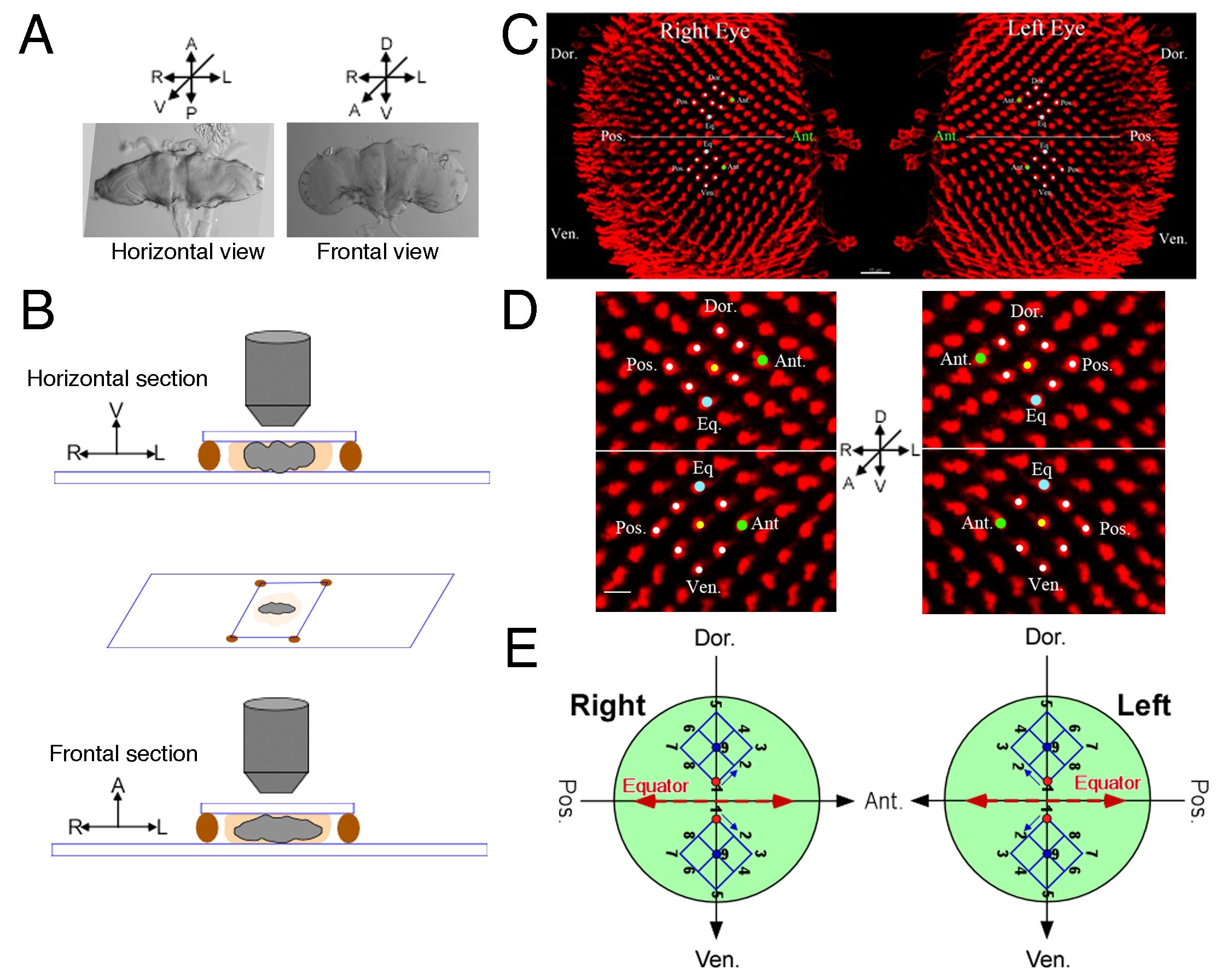
- To mount the brain in the horizontal orientation (Figures 1A, B), transfer the glycerol-cleared fly brain to a 20 µL drop of antifade mounting medium in the center of a slide.
- Attach small patches of clay at the 4 corners of the coverslip to prevent the coverslip from crushing the brain sample during mounting.
NOTE: The clay patches provide cushioning to prevent the coverslip from crushing the sample. Each clay patch should be about 1 mm in diameter. - Under a dissecting microscope, position the brains in the ventral-up position and place the coverslip on top to secure the brain. Use the convex dorsal surface of the brain as a landmark to identify the orientation of the brain sample (Figure 1A).
- Obtain the first image stack (horizontal view) with a confocal microscope. Use a high-NA objective lens (such as a 63X 1.3 N.A. glycerol or oil immersion objective lens) and 2.5X digital zoom (the pixel size is 0.105 µm per pixel; averaging number is 2). Acquire more than 180 optical sections (512 x 512 pixels) to cover the medulla neuropil with a step size of 0.2 µm.
- Remount the brain, but align the brain in the anterior-up position (frontal view).
- Acquire the second image stack (frontal view) of the same neuron.
NOTE: Finding the same neuron might be challenging when there are numerous neurons labeled in the optic lobe. To identify the same neurons from both orientations, lower-magnification image stacks from both views might be required (for example, use a zoom of 0.7, and a step size of 0.45 µm to acquire low-resolution image stacks). If the image is larger than 512 x 512, the image should be cropped to 512 x 512 before the image combination, and the pixel size should be kept at 0.105 µm per pixel while imaging the large field. Loss of signal is a potential problem for deep tissue. If the signal is weak, image the ventral half of the brain. To reduce photobleaching during scanning, use as low a laser power as possible. Use the range indicator to check for overexposure before acquiring image stacks. If possible, use a confocal microscope equipped with GaAsP detectors. - Identify and record the location of the neuron of interest with respect to the medulla neuropil (right/left [R/L] and dorsal/ventral [D/V]). Check if the sample moved during image acquisition by examining the image stack.
NOTE: Sample moving is often due to improper mounting. If sample movement occurs, the image stack cannot be used for registration and should be discarded. Re-mount the sample and acquire image stacks from the same neuron.
2. Image Deconvolution
NOTE: The deconvolution step uses image deconvolution software to restore the acquired images that are degraded by blurring and noise. While this step is optional, it significantly improves image quality.
- Start the deconvolution program in the interactive mode. Load the image stack (in lsm or specific microscopic format) by choosing Menu: File/Open (or Ctrl-o) in the main window.
- Click to select the loaded image stack and choose Menu: Ops to open the image operation window. Use the default Classic Maximum Likelihood Estimation (CMLE) algorithm.
- In the image operation window, click the "Parameters" tab. Enter the appropriate parameters for the lens immersion medium (e.g., oil, glycerin, etc.), embedding medium (e.g., immersion oil, etc.), and numerical aperture (NA; here, 1.3 was used). Check the remaining parameters to make sure that they correctly reflect the imaging conditions. Click the "Set all verified" tab to finalize the parameter settings.
- In the image operation window, click the "Operation" tab. Assign an output destination (e.g., c). Enter appropriate numbers in "Signal/Noise per channel" (e.g., "12 12 12 12" is a good starting point, while the default setting is "20 20 20 20"). Use default settings for the remaining parameters.
- Click the "Run Command" tab to start deconvoluting the image stack; depending on the computer, this process could take up to tens of minutes to complete.
- In the main window, click and select the deconvolved image stack. Choose Menu: Save As to save the deconvolved image in the ICS image file format (.ics and .ids).
NOTE: Each image stack has two files: the ics file contains the header informatio,n and the ids file contains the raw image information.- Rename the image stack files according to the imaging orientation (e.g., name the horizontal-view image stacks H.ids and H.ics and the frontal-view image stack F.ids and F.ics).
3. Dual-view Image Combination
NOTE: This step combines two image stacks to generate high-resolution 3D images using the MIPAV software.
- Generating matrices for image combination.
- Start the MIPAV program. Load the H and F image stacks by choosing Menu: File/Open image (A) from Disk (or Ctrl-f) /H.ids and F.ids; the window will show two images.
- Click the H image and choose Menu: Utilities/Conversion Tools/RGB/Grays; the window will show GrayG, GrayB, and GrayR images.
- Close GrayR and GrayB, only keeping GrayG on the window.
- Click the F image and choose Menu: Utilities/Conversion Tools/RGB/Grays. The window will show GrayG1, GrayB1, and GrayR1 images.
- Close GrayR1 and GrayB1 and keep only GrayG1 on the window. At this step, only GrayG and GrayG1 are on the window.
- Select the GrayG (highlight), and choose Menu: Algorithms/Registration/Optimized Automatic Image Registration; the "Optimized Automatic Image Registration 3D" dialog box will pop up.
- In the Input Options, change the "Degrees of freedom" from the default "Affine-12" to "Specific rescale-9." In "Rotations," key in -105 to 105 in the "Rotation angle sampling range" (default: -30 to 30 degrees), 10 in the "Coarse angle increment" (default: 15 degrees), and 3 in the "Fine angle increment" (default: 6 degrees).
- Click OK. The first Matrix, "GrayG_To_GrayG1.mtx," will be generated and saved in the image folder. Close all the image windows and proceed to the next step, which will take at least 15 minutes.
- Load the H and F image stacks by choosing Menu: File/Open image (A) from Disk (or Ctrl-f) /H.ids and F.ids.
- Select the H image by clicking the image and choose Menu: Utilities/Conversion Tools/RGB/Gray; the "RGB->Gray" dialog box will pop up. Click OK; the window will show "HGray" images. Keep HGray and close the H image.
- Repeat step 3.1.9 for the F image; the "FGray" images will appear in the window. Keep FGray and close the F image; only HGray and FGray will be left on the window.
- Select the HGray image (highlight) and go to Menu: Algorithms/Transformation tools/Transform. The "Transform/Resample Image" dialog box will pop up. Click the "Resample" tab and change the resample to size of "HGray" to "FGray". Next, click the "Transform" tab and load "GrayG_To_GrayG1.mtx" by selecting the "Read matrix from file." Click OK; the window will show the HGray_transform image. Close the HGray image so only HGray_transform and FGray are left on the window.
- Select the "HGray_transform" image (highlight) and go to Menu: Algorithms/Registration/Optimized Automatic Image Registration. The "Optimized Automatic Image Registration 3D" dialog box will pop up. In "Rotations," key in -5 to 5 in the "Rotation angle sampling range" (default: -30 to 30 degrees), 3 in the "Coarse angle increment" (default: 15 degrees), and 1 in the "Fine angle increment" (default: 6 degrees). Click OK.
NOTE: The Affine Matrix (HGray_transform_To_FGray.mtx) will be generated and saved in the image folder, and the "HGray_Transform_register" image will be shown on the window. This step will take at least 40 min. - Close the "HGray_transform" image; only "HGray_Transform_register" and "FGray" should be left on the window.
- Select the "HGray_Transform_register" image (highlight) and go to Menu: Algorithms/ Registration/B-Spline Automatic Registration 2D/3D. The "B-Spline Automatic Registration-3D intensity" dialog box will pop up. Select "Least Squares" in the Cost function (the default is Correlation Ratio).
- Click "Perform two-pass registration". In the Pass 1 section, key in 2 into "Gradient Descent Minimize Step Size (sample units)" (the default is 1) and key in 10 into "Maximum Number of Iterations:" (the default is 10). In the Pass 2 section, key in 1 into "Gradient Descent Minimize Step Size (sample units)" (the default is 0.5) and key in 2 into "Maximum Number of Iterations:" (the default is 10).
NOTE: The NLT matrix, "HGray_transform_register.nlt," will be saved in the image folder, and the "HGray_transform_register_registered" image will be shown on the window. This step will take at least 5 min.
- Close all the images on the window.
- Generating the reference image for image combination.
NOTE: This step is meant to generate a registered horizontal image for combination.- Load H and F image stacks by choosing Menu: File/Open image (A) from Disk (or Ctrl-f) /H.ids and F.ids; two images will appear on the window.
- Select the H image (highlight) and go to Menu: Algorithms/Transformation tools/Transform; the "Transform/Resample Image" dialog box will pop up. Click the "Resample" tab and change the resample from a size of "H" to "F." Next, click the "Transform" tab and load "GrayG_To_GrayG1.mtx" by selecting "Read matrix from file." Click OK; the H_transform image will appear on the window. Close the H image but keep H_transform and F in the window.
- Select the "H_transform" image (highlight) and go to Menu: Algorithms/Transformation tools/Transform; the "Transform/Resample Image" dialog box will pop up. Click the "Resample" tab and change the resample from a size of "H_transform" to "F." Next, click the "Transform" tab and load "HGray_transform_To_FGray.mtx" by selecting "Read matrix from file." Click OK; the "H_transform_transform" image will appear on the window. Close the H_transform image; at this point, only H_transform_transform and F will be left on the window.
- Select the "H_transform_transform" image (highlight) and go to Menu: Algorithms/Transformation tools/Transform nonlinear; the "Nonlinear B-Spline Transformation" dialog box will pop up. Next, load "HGray_transform_register.nlt" and click OK; the "H_transform_transform_registered" image will appear on the window. Save the image as an ics file. Close all the images on the window.
- Combining image stacks
NOTE: This step combines two image stacks acquired in orthogonal orientations (horizontal and frontal) into one high-resolution stack.- Go to Menu: Plugins/Generic/Drosophila Retinal Registrationl; the "Drosophila Retinal Registration v2.9" dialog box will pop up. Upload "H.ics" in image H, "H_transform_transform_registered" from step 3.2.4 in Image H-Registered, "F.ics" in Image F, "GrayG_To_GrayG1.mtx" from step 3.1.7 in Transformation 1-Green (optional), "HGray_transform_To_FGray.mtx" from step 3.1.12 in Transformation 2-Affine, and "HGray_transform_register.nlt" from step 3.1.14 in Transformation 3-Nonlinear (optional).
- Select SqRt(Intensity-H x Intensity-F) and No rescale in "Rescale H to F." Keep the default options for the remaining parameters. Click OK; this step will take about 3 min.
NOTE: After processing, 3 sets of images will be generated: combinedImage_sqrRt_trilinear_norescale_ignoreBG.ids (the final recombined image), greenChannelsImage-Gxreg-Gy-Gcomp.IDS (green channel for H, F, and the final recombined image), and redChannelsImage-Rxreg-Ry-Rcomp.ids (red channel for H, F, and the final recombined image); all the output files will be resized to 512 x 512 x 512.
- Open "combinedImage_sqrRt_trilinear_norescale_ignoreBG.ids" under the image visualization software. Save the image stack in the ims format and rename the file; this recombined image file will be used for neurite tracing and registration.
4. Neurite Tracing and Reference Point Assignment
NOTE: This step involves tracing neurites (4.1) and assigning reference points for registration (4.2) using the image visualization software.
- Tracing neurites
- Start the image visualization software. Open the recombined image file. Go to Menu: Edit/Show Display Adjustment and turn off the photoreceptor channel (red).
- Visualize the image in "Surpass" mode. If the computer is equipped with a stereograph system, turn on "stereo" and use the "Quad Buffer" mode to visualize 3D images.
- Go to Menu: Surpass/Filaments to add new filaments. Click the "Skip automatic creation, edit manually" tab.
- Click the "Draw" tab and select "AutoDepth."
- Select "Settings," check "Line," and key in an appropriate pixel number for better visualization (a 4-pixel line is used in this protocol). Check "Show Dendrites," "Beginning Point," and "Branching Points". Set "Render Quality" to 100%.
- Select the "Draw" tab and start tracing neurites. Start with the axon and then move to the dendrites (Figure 1D). The axon and dendrites of transmedulla neurons are easy to differentiate.
NOTE: A Tm neuron extends its axon from the cell body and projects all the way to the higher visual processing center, the lobula. The system will automatically define the first long filament as an axon and the remaining short filaments as dendrites. Keep the starting point at the beginning of the filament (axon) during tracing, and make sure that the traced neurites are connected. Examine the branching points and the beginning point. If the dendrites are not connected, a new beginning point will be defined at the non-connected filament. - After tracing, go back to "Settings," uncheck "Beginning Point" and "Branching Point," and go to Menu: Surpass/Export selected objects../. Save the filament as an inventor file (*.iv).