Investigations on Alterations of Hippocampal Circuit Function Following Mild Traumatic Brain Injury

Summary

A multi-faceted approach to investigating functional changes to hippocampal circuitry is explained. Electrophysiological techniques are described along with the injury protocol, behavioral testing and regional dissection method. The combination of these techniques can be applied in similar fashion for other brain regions and scientific questions.

Abstract

Traumatic Brain Injury (TBI) afflicts more than 1.7 million people in the United States each year and even mild TBI can lead to persistent neurological impairments ¹. Two pervasive and disabling symptoms experienced by TBI survivors, memory deficits and a reduction in seizure threshold, are thought to be mediated by TBI-induced hippocampal dysfunction ^2,3. In order to demonstrate how altered hippocampal circuit function adversely affects behavior after TBI in mice, we employ lateral fluid percussion injury, a commonly used animal model of TBI that recreates many features of human TBI including neuronal cell loss, gliosis, and ionic perturbation ^4-6.

Here we demonstrate a combinatorial method for investigating TBI-induced hippocampal dysfunction. Our approach incorporates multiple ex vivo physiological techniques together with animal behavior and biochemical analysis, in order to analyze post-TBI changes in the hippocampus. We begin with the experimental injury paradigm along with behavioral analysis to assess cognitive disability following TBI. Next, we feature three distinct ex vivo recording techniques: extracellular field potential recording, visualized whole-cell patch-clamping, and voltage sensitive dye recording. Finally, we demonstrate a method for regionally dissecting subregions of the hippocampus that can be useful for detailed analysis of neurochemical and metabolic alterations post-TBI.

These methods have been used to examine the alterations in hippocampal circuitry following TBI and to probe the opposing changes in network circuit function that occur in the dentate gyrus and CA1 subregions of the hippocampus (see Figure 1). The ability to analyze the post-TBI changes in each subregion is essential to understanding the underlying mechanisms contributing to TBI-induced behavioral and cognitive deficits.

The multi-faceted system outlined here allows investigators to push past characterization of phenomenology induced by a disease state (in this case TBI) and determine the mechanisms responsible for the observed pathology associated with TBI.

Protocol

1. Lateral Fluid Percussion Injury

1. Anaesthetize the mouse using a mixture of ketamine and xylazine given intraperitoneally. Then prepare the mouse's head for incision using an iodine scrub.
2. Perform a craniectomy over the right parietal area using 3 mm (outside diameter) trephine.
3. Secure Luer-loc needle hub (inside diameter 3 mm) over the craniectomy using cyanoarylate and dental acrylic.
4. 24 hr later, anaesthetize the mouse using isoflurane via inhalation.
5. Once normal breathing resumes, but before the mouse becomes sensitive to stimulation, deliver 20 msec pulse of saline into the skull via the fluid percussion injury device.
6. Immediately after injury remove the hub, reanaesthetize the mouse using isoflurane, and suture the scalp closed.
   Sham-operated controls will receive an identical procedure with step 1.5 omitted.

2. Behavioral Analysis - Conditioned Fear Response

1. Handle mice on two consecutive days prior to conditioned fear response (CFR) training.
2. Place mouse in conditioning chamber for 3 min before administering 1.5 mA floor shock for 2 sec. Leave mouse in chamber for an additional 30 sec.
3. After delay period (usually 24 hr), return mouse to conditioning chamber for 5 min. Assess freezing at 5 sec intervals.
   Analysis consists of comparing the relative amount of time freezing in two populations, in our case brain-injured mice and sham-operated controls. Lower freezing rates (compared to control) indicate inability to retain the association between the context and the floor shock, an indication of memory impairment and cognitive dysfunction.

3. Preparing Acute Hippocampal Slices

*Note: Anesthetization using a Bell Jar can only be implemented for terminal procedures (such as the brain dissection described herein).

1. 7 days after injury, make 1 L of artificial cerebral spinal fluid (aCSF) and 250 ml sucrose cutting solution.
2. Use ice liberally to ensure that all instruments and solutions used during brain slice preparation are ice cold.
3. Anaesthetize mouse using isoflurane. Quickly and gently remove brain from mouse and place in sucrose.
4. Trim brain and place on cutting surface on a drop of superglue in front of an agar block.
5. Cut 350 μm thick coronal slices, you should be able to get 4 or 5 slices with the intact hippocampal circuit.
6. Incubate slices for at least 1 hr at 37 °C.

4. Extracellular Field Potential Recording

1. Pull borosilicate glass electrodes to 2-5 MΩs using vertical puller.
2. Place slice in chamber and insert electrode onto electrode holder.
3. Lower stimulating electrode into slice in an axonal tract such as the perforant path or Schaffer collaterals. Lower recording electrode into position while monitoring output traces to ensure that electrodes are at the same z-level (depth). When a maximal response is achieved, holding stimulation current level constant, electrodes are at the same z-level.
4. The resultant trace consists of three components: the presynaptic fiber volley, the field extracellular postsynaptic potential (fEPSP), and the postsynaptic population spike. The components may overlap temporally in some preparations, making analysis more difficult. If there is ambiguity between whether responses are presynaptic or postsynaptic, APV and CNQX can be added to the bath to block excitatory transmission, and all remaining signals will be of presynaptic origin.
5. Stimulation protocols vary to produce three distinct experiment types: input/output curves, paired pulse recordings, and long-term plasticity experiments.
   Analysis typically consists of measurements comparing the slope of the fEPSP across in both brain-injured mice and sham-operated controls, controlling for the input strength by measuring the fiber volley.

5. Visualized Patch-clamp Recording

1. Prepare slices, electrodes, and rig to record as previously described above up to step 4.2.
2. Only consider cells deeper than 80 μm into the tissue as cells nearer the surface will be dead and/or have reduced connectivity. Approach a cell with positive pressure on the electrode to ensure that it does not get clogged as it moves down through the tissue. When the electrode gently touches the cell apply negative pressure in order to create a 'gigaseal' between the electrode and the plasma membrane.
3. Apply short bursts of negative pressure in order to rupture the plama membrane under the electrode and achieve whole-cell configuration.
4. Eliminate capacitance transients using amplifier and compensate for series resistance. Compensating for the series resistance of the cell is essential to ensure accurate measurements.
5. Two modes of single cell recordings can be performed: current clamp (measuring membrane voltage) and voltage clamp (measuring current passing through ion channels in the membrane).
   Possible types of analysis are numerous but in our case mostly consist of biophysical analysis quantifying the rate and size of spontaneous synaptic currents in both brain-injured mice and sham-operated controls.

6. Voltage Sensitive Dye Imaging (VSD)

1. Prepare slices and rig to record as previously described above up to step 4.2.
2. Prepare dye stock by mixing 1 mg di-3-ANEPPDHQ into 50 μl ethanol; dispense 2 μl aliquots into foil wrapped tubes, store at -20 °C. Make working dye solution daily, by diluting 1:200 in aCSF.
3. Incubate slice on aCSF moistened filter paper and stain with 90 μl of dye for 16 min; rinse with aCSF and place in interface recording chamber.
4. Adjust light stimulation intensity until response is centered in middle of camera range. Images are typically acquired at a rate of 500-1,000 frames per second.
5. Trigger shutter for light stimulation 200 msec before electrical stimulation to allow initial rapid photobleaching to stabilize. Alternate acquisition trials between electrically stimulated, and non-electrically stimulated, to allow later subtraction of non-stimulated background. Record resting light intensity (fluorescence reading with shutter closed) prior to opening shutter. Each VSD trial will be an x pixels by y pixels by time "movie" of fluorescence readings. Record 10 - 12 VSD trials in each test condition.
6. All measurements are performed on the intra-pixel pre-electrical-stimulus normalized fluorescence change, dF/F, which is calculated as follows:
   Subtract the resting light intensity from the VSD raw acquired trial. For each pixel in each trial, normalize according to the pre-electrical-stimulus mean value for that trial, and subtracting unity. Do this for both the electrically stimulated and non-electrically stimulated trials. Create an average "background fluorescence" trial from the non-electrically stimulated trials, and subtract this background trial from the electrically stimulated trials. Further analysis is typically performed on the average of 10 - 12 such trials, which are also usually filtered in space and time to improve the signal to noise ratio.

7. Regional Dissections for Biochemical Analyses

1. Remove the brain from the mouse as previously described.
2. Prepare slices using tissue chopper.
3. Lay section flat, microdissect area CA1 and DG.
4. Immediately immerse in lysis buffer containing protease inhibitor. Freeze in liquid nitrogen and store at -80 °C.

8. Representative Results

Our experiments typically begin with behavioral data to confirm the expected cognitive deficits that exist in brain-injured mice. We employ contextual conditioned fear response testing as it is a hippocampal dependent behavior that is reliable and requires only one training session and one testing session. The data depicted in Figure 2 represents behavioral testing to measure anterograde memory; however, the test can also be used to measure retrograde memory if the training session is performed before the injury.

Field excitatory postsynaptic potentials (fEPSPs) are measured to determine the net synaptic efficacy of a large population of cells (Figure 3A). We commonly employ three different types of stimulation patterns, each affording its own results and conclusions. First, by increasing the stimulation intensity through a series of steps, we create an input/output curve (Figure 3B/C).

Next, by delivering two stimulations of the same intensity separated by a brief delay (usually 50 msec) we investigate potential alterations in synaptic vesicle release probability.; Additionally, we often perform long-term potentiation (LTP) experiments. After establishing a baseline response, brief high frequency stimulation (usually 100Hz) at the same intensity is delivered, causing an intracellular cascade that leads to a potentiated synaptic response when normal stimulation is resumed.

Electrical activity from whole-cell patch-clamped cells can be recorded in two modes. In voltage clamp mode, the experimenter controls the membrane voltage of the patch-clamped cell in reference to the bath, via computer software associated with the amplifier. In this case currents mediating postsynaptic events are recorded, providing information about presynaptic release frequency, number of postsynaptic receptors activated and vesicular neurotransmitter concentration (Figure 4A). In current clamp mode the experimenter manipulates injected current and measures the voltage response. This can be useful to determine characteristics of the action potential, such as action potential threshold and half-width. These characteristics allow for the functional categorization of neurons as excitatory or inhibitory based on their action potential firing patterns (Figure 4B). In order to verify the cellular identity we recommend filling cells with Lucifer Yellow after recording and visually confirming identity by the presence or absence of dendritic spines. (Figure 4C, D).

An example of results from an experiment using voltage sensitive dye to measure changes in membrane voltage is depicted in Figure 5. In this case, a stimulating electrode has been placed in the Schaffer collateral pathway and the resulting neuronal activity in area CA1 is analyzed. Voltage sensitive dye does not report absolute values of membrane voltage, but rather the change in voltage from a baseline condition without stimulation. However, analyses comparing two conditions (e.g. brain-injured vs. sham-operated) can be used to determine the spatiotemporal parameters of physiological alterations that cannot be measured using fEPSPs or whole-cell patch-clamp recording.

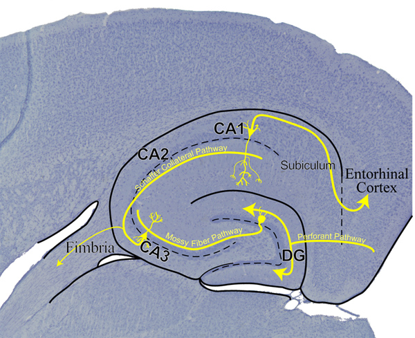
Figure 1. Hippocampal Circuit Diagram. A horizontal section through the hippocampus. The major pathways through the hippocampus are shown in yellow. The axons from neurons in the entorhinal cortex project via the perforant pathway into the dentate gyrus forming synapses with the dendrites of dentate gyrus granule cells. Granule cell axons project via the mossy fiber pathway to CA3 where they form synapses with the dendrites of CA3 neurons. The axons of CA3 neurons project via the Schaffer collateral pathway onto the dendrites of CA1 pyramidal cells. The axons of CA1 pyramidal cells project out of the hippocampus through the subiculum. Note: Also depicted are CA3 pyramidal cell axon collaterals projecting to the contralateral hippocampus via the fimbria. (CA1: Cornu Ammonis 1, CA2: Cornu Ammonis 2, CA3: Cornu Ammonis 3, DG: Dentate Gyrus, dashed line indicates cell body layer, solid line indicates structural boundaries.)

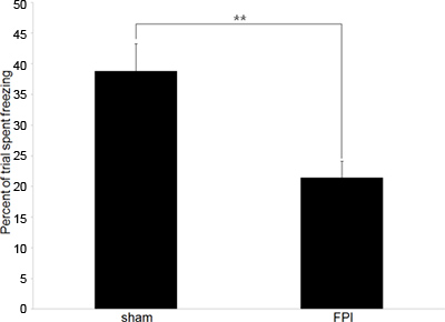
Figure 2. Representative Behavioral Data. A: Behavioral data depicting the difference in freezing rates between brain-injured mice (FPI) and sham-operated controls (sham) in the conditioned fear response paradigm. Training occurred on the 6^th day following injury, with the test period occurring 24 hr later. (** denotes p<.01.)

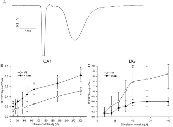
Figure 3. Representative Extracellular Recording Data. A: An example of a field excitatory post-synaptic potential (fEPSP) recording in area CA1. The first downward deflection is the stimulus artifact, followed by the presynaptic fiber volley and finally the fEPSP. B: Input/output curves depicting a decrease in net synaptic efficacy in CA1 following fluid percussion injury (FPI). C: Input/output curves depicting an increase in net synaptic efficacy in dentate gyrus (DG) following FPI. (* denotes p<.05.) Click here to view larger figure.

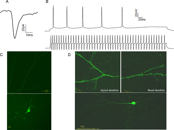
Figure 4. Representative Whole-cell Patch-clamp Data. A: An example spontaneous excitatory postsynaptic current (sEPSC) from a CA1 pyramidal cell. B: Examples of action potential trains from a CA1 pyramidal cell (upper trace) and a fast spiking CA1 interneuron (lower trace). C: Example of a Lucifer Yellow filled CA1 inhibitory interneuron. Note the absence of dendritic spines (upper panel). D: Example of Lucifer Yellow filled CA1 pyramidal neuron. Note the presence of dendritic spines (upper panel). Click here to view larger figure.

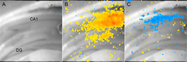
Figure 5. Representative Voltage Sensitive Dye Imaging Data. A: Mouse coronal hippocampal slice displayed to show anatomy. (DG: dentate gyrus, CA1: Cornu Ammonis 1) B: Yellow to red pixels representing excitatory activity in area CA1 14 msec after afferent Schaffer collateral stimulation. Red indicates more depolarization while yellow indicates a lower, but still significant depolarization. C: Blue pixels representing sites of inhibitory activity in area CA1 56 msec after the same afferent Schaffer collateral stimulation shown in B. Darker blue indicates more hyperpolarization.

Discussion

Each technique outlined above contributes to the greater understanding of the underlying mechanism causing the observed behavioral deficit. By combining the unique information gained from each method we are able to examine the biological mechanisms with more precision.

Measuring fEPSPs is useful for quantifying the net synaptic efficacy of large, spatially defined regions of neurons. It also can provide information about the potential of a group of cells to undergo synaptic plasticity, a ne...

Materials

List of materials used in this article

Name	Company	Catalog Number	Comments
Axopatch 200B amplifier	Molecular Devices	AXOPATCH 200B	Patch-clamp rig
Digidata 1322A digitizer	Molecular Devices		Patch-clamp rig
MP-225 micromanipulator	Sutter	MP-225	Patch-clamp rig
DMLFSA microscope	Leica		Patch-clamp rig
Multiclamp 700B amplifier	Molecular Devices	MULTICLAMP 700B	Multipurpose (field) rig
Digidata 1440 digitizer	Molecular Devices		Multipurpos (field) rig
MPC-200 micromanipulator	Sutter	MPC-200	Multipurpose (field) rig
BX51WI microscope	Olympus	BX51WI	Multipurpose (field) rig
Axoclamp 900A amplifier	Molecular Devices	AXOCLAMP 900A	VSD rig
Digidata 1322 digitizer	Molecular Devices		VSD rig
Redshirt CCD-SMQ camera	Redshirt	NCS01	VSD rig
VT 1200S Vibratome	Leica	14048142066
P-30 Electrode puller	Sutter	P-30/P
cOmplete protease inhibitor	Roche	11697498001