ScanLag: High-throughput Quantification of Colony Growth and Lag Time

Summary

ScanLag is a high-throughput method for measuring the delay in growth, namely lag time, as well as the growth rate of colonies for thousands of cells in parallel. Screening using ScanLag enables the discrimination between long lag-time and slow growth at the level of a single variant.

Abstract

Growth dynamics are fundamental characteristics of microorganisms. Quantifying growth precisely is an important goal in microbiology. Growth dynamics are affected both by the doubling time of the microorganism and by any delay in growth upon transfer from one condition to another, the lag. The ScanLag method enables the characterization of these two independent properties at the level of colonies originating each from a single cell, generating a two-dimensional distribution of the lag time and of the growth time. In ScanLag, measurement of the time it takes for colonies on conventional nutrient agar plates to be detected is automated on an array of commercial scanners controlled by an in house application. Petri dishes are placed on the scanners, and the application acquires images periodically. Automated analysis of colony growth is then done by an application that returns the appearance time and growth rate of each colony. Other parameters, such as the shape, texture and color of the colony, can be extracted for multidimensional mapping of sub-populations of cells. Finally, the method enables the retrieval of rare variants with specific growth phenotypes for further characterization. The technique could be applied in bacteriology for the identification of long lag that can cause persistence to antibiotics, as well as a general low cost technique for phenotypic screens.

Introduction

Bacteria have evolved to respond to many stressful conditions. A general feature of adaptation to stress is a change in growth dynamics^1,2. Growth dynamics are characterized mostly by two parameters: the exponential growth rate and the lag time, namely the time needed to adapt to new conditions. Whereas a large number of high throughput methods focus on measurements of the growth rate, the lag time is often an overlooked parameter, although it is the crucial parameter for characterization of the adaptation to new conditions. Quantification of the adaptation to changing conditions has traditionally been performed using laborious manual methods^3,4. More recently, advanced techniques have been developed for analysis of single cells^5,6. However, it is still difficult to distinguish normal growth following a delay in growth (namely a lag time)^2,3 from slow growth. An automated method was constructed, ScanLag⁷, to discriminate between these two similar phenotypes.

A striking example of the importance of the study of the lag time distribution is revealed under antibiotic treatment. Many antibiotics and other stresses kill only actively growing cells, and, therefore, cells that are “lagging” are protected⁸. To monitor lag time, one can observe single cells under a microscope and monitor the time to first division. A major drawback of this method is that the dynamic time range is limited; those cells that are growing early cover the surface at an exponential rate, effectively decreasing the growth of cells with longer lag time. Use of flow chambers somewhat circumvents this⁵, but a limited number of cells can be tracked and the fraction of bacteria that exit the lag phase after the majority of the population has started growing cannot be observed. Despite these limitations, several studies have evaluated the influence of the level of different stresses on lag time distribution using single cell microscopy^9-12. Another way to monitor lag time distribution is through turbidity measurements^13,14. Many parallel cultures, each started from a single cell, are grown in an optical density reader that measures the number of bacteria in the culture over time. This method is limited by the precision of the extrapolation and to the number of wells in a plate.

An automated method was developed, called ScanLag, that enables lag times and growth time distributions to be assessed, even for the small percentage of bacteria in a population that have very long lag times. The method is based on detection of colonies on conventional nutrient agar plates¹⁵ (Figure 1). To automate detection^16,17 an array of commercial scanners¹⁸ that are directed by in house software to periodically acquire images of the plates, was engineered. Software was designed to automatically analyze the images and extract quantitative parameters^19,20, such as time of appearance of each colony and growth time of each colony, which is defined here as the time to grow from 20 pixels to 80 pixels. Here we present the method in detail, including the setup of the system and the use of the automated image analysis software which has been improved with a better user interface.

This method can be adapted to measure other characteristics of colonies, such as morphology and color. Measurement of these types of parameters will allow the system’s use in multidimensional phenomics. As the method detects colonies from single cells, the system can reveal new phenotypes that cannot be measured by population-level measurements. The technique enables the detection and retrieval of rare variants, and facilitates screening for desired traits.

Protocol

1. Build the Setup

1. Choose a flatbed Scanner with optical resolution: 4,800 dpi; Hardware resolution: 4,800 x 9,600 dpi; color bit depth: 48 bit, that can operate at the relevant temperature and humidity levels.
2. Petri dishes have significant volume, unlike paper usually used on commercial scanners. The colonies lie on top of the agar layer, about 5 mm above the scanner surface. Note: For most scanners the colonies will be in focus.
3. Some scanner companies do not allow connection of more than one instance of scanner of the same type to the same computer. Make sure that more than one scanner can be attached and identified uniquely.
4. Prepare the accessories as detailed below:
   1. Prepare pieces of sterile black felt cloth to cover the plates (Figure 1 step 2).
   2. To hold the Petri dishes in place, prepare white plate holders (Materials and Methods) that fit the scanners and that have 6 holes the size of the dishes (Figure 1 step 3).
5. If needed for the growth of the microorganism, put the scanners in a temperature controlled environment. Connect the scanners to the computer.
6. Optional: Connect the relay to the computer and bypass the on/off switch of the scanner to overcome temperature gradient.
   NOTE: The relay unit is for extremely temperature sensitive microorganisms. It switches off the scanner so that the electronics do not heat the surface unevenly. Using only part of the scanner surface may achieve similar results.

2. Install the Scanning Manager

1. Copy all 'Scanning Manager' application files into a designated directory from http://www.phys.huji.ac.il/bio_physics/nathalie/publications.html.
2. Configure ScanningManager.exe.config file according to the scanners names as they appear in Computer Management->Device Manager->Imaging Devices (Figure 2).
3. For troubleshooting of the 'Scanning Manager' application, see the read me file.
4. For further documentation on the 'Scanning Manager' application, see Documentation.html.

3. Perform an Experiment

1. Prepare the Petri dishes (Figure 1):
   1. Dilute the culture to approximately 2,000 CFU/ml. Plate 0.1 ml of culture uniformly on the plate surface.
   2. To gain good contrast between the colonies and the dish and to absorb moisture, cover the plate with a piece of sterile black felt cloth. Put lid on the plate.
2. Place the plates in the holders on the scanners.
3. Start the Scanning Manager (Figure 3): Choose the participating scanners from the list of attached scanners. Choose the number of images to be taken (Repetitions), the time interval between subsequent images (Time gap), and the time delay before starting the experiment (Start After).

4. Analysis of the Images

NOTE: An outline of computational methods is provided for analyzing the images in MATLAB using “ScanLag”, which is freely available for non-commercial use at http://www.phys.huji.ac.il/bio_physics/nathalie/publications.html. Further functions available are detailed in the software manual, and an example code is supplemented.

1. Sort the images from each scanner into separate folders.
2. Using Matlab’s command window, run the following procedures. The parameters required to run these procedures are defined in the software manual.
   1. Run PreparePictures to perform preprocessing: In preprocessing, the images from a scanner are aligned. Each Petri dish is cropped from each sequence of images. The time at which each image was collected is retrieved from the timestamp.
   2. Run TLAllPlates to perform detection and tracking In each Petri dish separately, colonies are detected and assigned an identifying number.
   3. Analysis of the extracted data: The sizes of every detected colony are measured as a function of time. To extract the appearance distribution of the colonies use the following functions in Matlab’s command window (further information is available in the software manual):
      1. Run ScanLagApp to display the analysis of a certain Petri dish alongside with the graph of the colonies size versus time (Figure 4).
         1. Use the slider to change the current time of the plate. The timing will also be indicated by a matching vertical line on the colonies area graph.
         2. Click on a colony to see its associated curve, and vice versa, click on a curve to find its associated colony. After identifying the colony, the phenotype can be retrieved by picking the colony from the identified Petri dish.
         3. Filter defects in the automatic analysis by choosing a colony and clicking the exclude button. When clicking exclude the number of the colony will turn yellow.
      2. After going through the results of the analysis of each plate, sum up the results:
         1. Run AddHistograms to create a histogram of appearance times.
         2. Run plotDeathCurve to create a survival curve representation of the distribution.
         3. Run GetAppearanceTimes to get the appearance time of all colonies in the experiment.

Results

As an example of lag time distribution extraction, Figure 5 shows the ability of ScanLag to identify and track each colony with specific characteristics on one plate over time, as would be done in a screening assay.

When the culture of the microorganism is heterogeneous, the different subpopulations might reveal themselves during the assay. For example, Figure 6 shows the appearance quantification and thus reveals bimodal lag time distribution in a mutant strain of E. coli.

The growth rate of the cells influences the appearance time of the colony. When colonies grow at the same rate, the late appearance can be attributed to the lag time (Figure 7).

To validate that the method indeed measures the lag time of single cells, we compared ScanLag results with those obtained using single-cell microscopy; this validation is described in detail in a previous publication⁷. This method enables monitoring of many more cells than can be evaluated with microscopy. The distributions obtained using microscopy and obtained using ScanLag largely overlap. The ScanLag distribution is slightly broader; theoretical analyses predict broadening to be of the order of the standard deviation of the division time. If growth time is different for each strain, the origin of the delay in appearance must be further investigated using other methods.

The influence of early-appearing colonies on the appearance of later colonies was examined. Control experiments⁷ confirmed that later appearance was not affected as long as the total number of colonies per plate did not exceed 200 (Figure 8). Another control experiment confirmed that the location of the colony on the plate was not affecting its appearance time ⁷.

The analysis of the plates is calibrated to specific thresholds that might need modification depending on nutrients present in growth medium or the type of microorganism. Nevertheless, the analysis is quite robust for a large range of thresholds as shown in Figure 9.

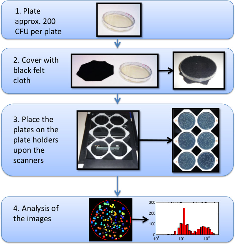
Figure 1. A schematic diagram of the steps needed to create a colony appearance distribution.

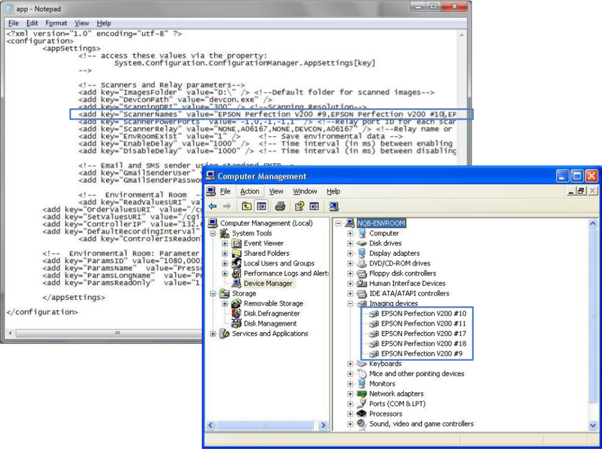
Figure 2. A screen shot of the Device Manager showing the names of the attached scanners, and of the configuration file. Please click here to view a larger version of this figure.

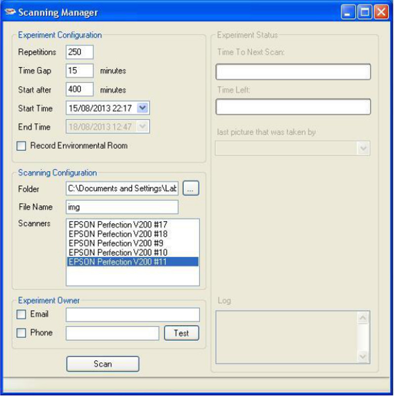
Figure 3. A screen shot of the Scanning Manager.

Figure 4. A screen shot of the ScanLagApp. An image of the plate is on the left pane, and the growth curves of each colony are on the right pane, as detailed in the manual. The spikes in some of the colonies area curves occur when two or more colonies merge. When merging of colonies happens, the area of these colonies is considered as the joint area.

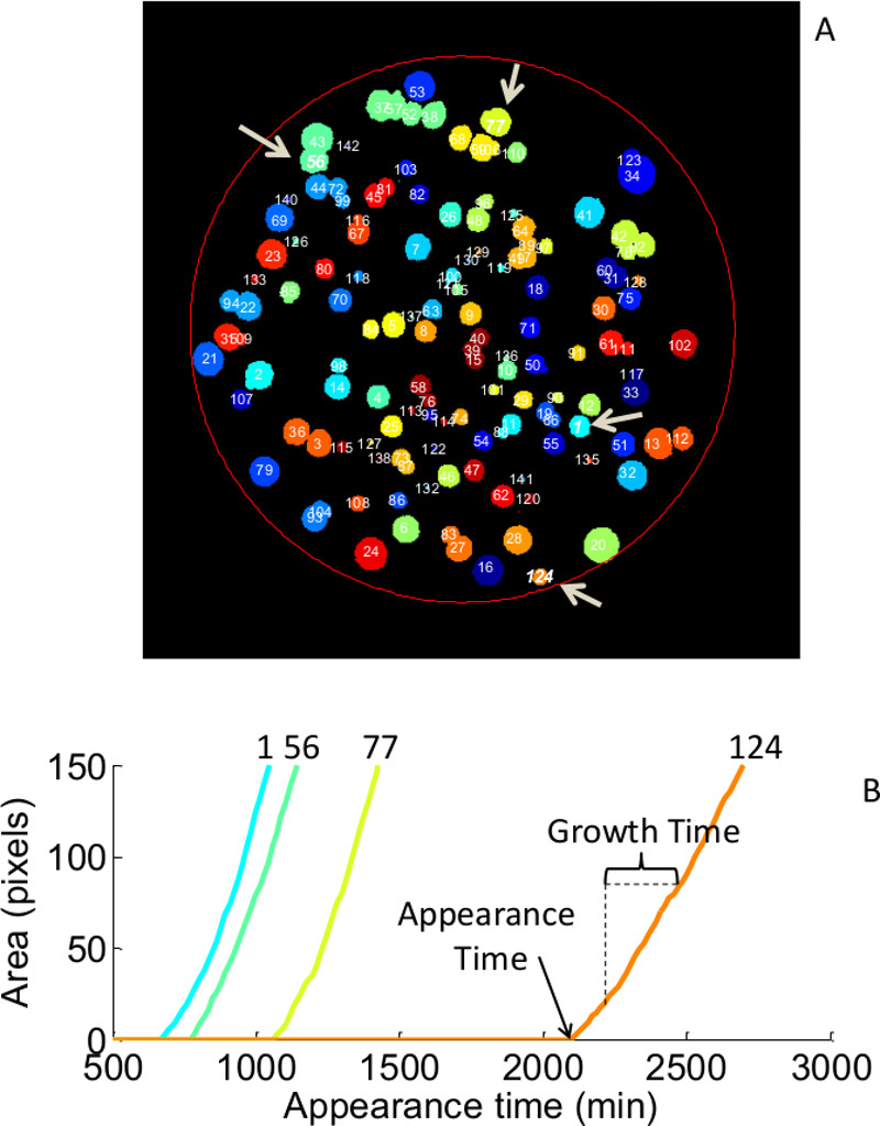
Figure 5. A representative result of the analysis of one plate. (A) An image of the output of the detection application at the end of the experiment. Each colony area is identified, colored and assigned with a unique ID number. The arrows point to representative colonies measured in B. The colony is detected based on intensity threshold (For E. coli colonies on LB agar or M9 agar this threshold is 0.03. For other media or bacteria, this threshold can be adjusted in the function ProcessPictures). Only objects above 10 pixels are counted (this threshold can be modified in the function MatchColonies). Detection of a colony starts at approximately 10⁵ bacteria. (B) Plots of the area in pixels versus time of four representative colonies in this plate. The ‘appearance time’ of each colony is when the colony is detected. The ‘growth time’ of each colony is defined here as the time to grow from 20 pixels to 80 pixels (those boundaries are adjustable using the function getAppearanceGrowthByVec). The software excludes the colonies that merged before reaching the upper bound. Identification of a specific colony according to its characteristics is easy thanks to the identifying number and the color assigned to each colony. For example colonies # 1, 56, 77 and 124 are highlighted in both graphs.

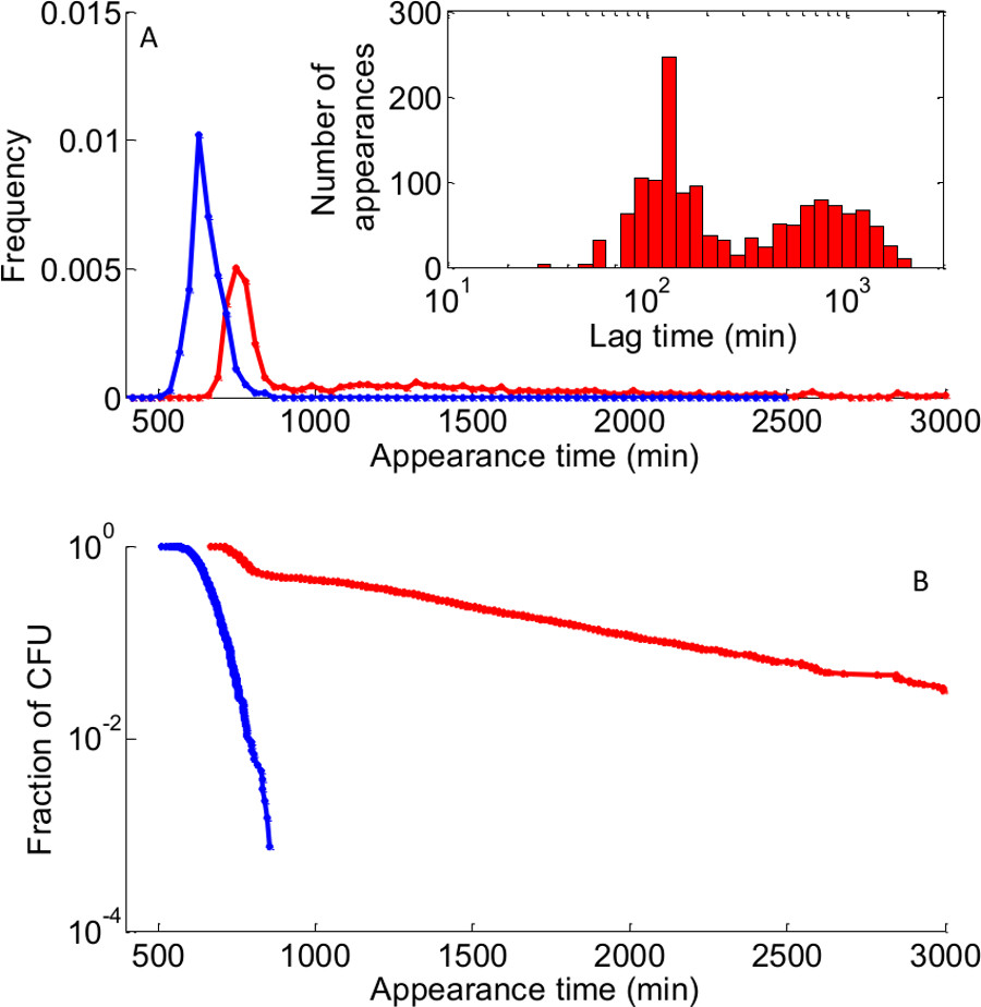
Figure 6. Appearance quantification can reveal bimodal lag time distribution. Comparison of ScanLag analysis histograms of appearance times for two different strains. Blue line: wild type strain exponentially growing (Total: 1,320 colonies); red line- high persistence mutant enriched with lagging bacteria (Total: 1,529 colonies). (A) Normalized appearance histograms. The peak of appearance of exponentially growing cells is the typical time to grow to a detectable colony. Inset: same histogram of the mutant strain after subtracting the time of the peak of the exponential culture to get the actual lag time on log-spaced bins showing the bimodal lag time distribution. (B) Survival function of the same data as in (A) on a logarithmic scale. This representation enhances the late appearance tail of the mutant strain.

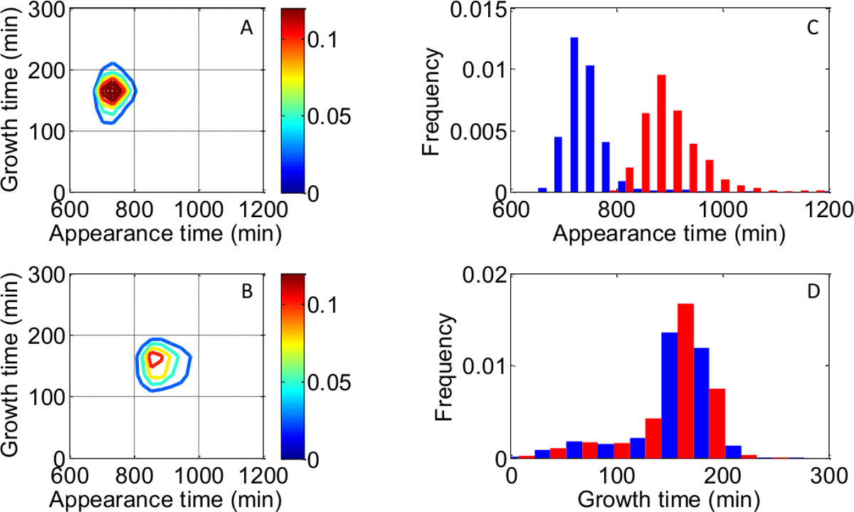
Figure 7. Appearance distribution and growth time distribution. (A) and (B) show two dimensional histograms of the appearance time and the growth time of the two different conditions (The software excludes colonies that merged before reaching the upper bound). (C) Comparing the histograms of the two strains show the difference in appearance time, whereas the growth times (D) are similar. Please click here to view a larger version of this figure.

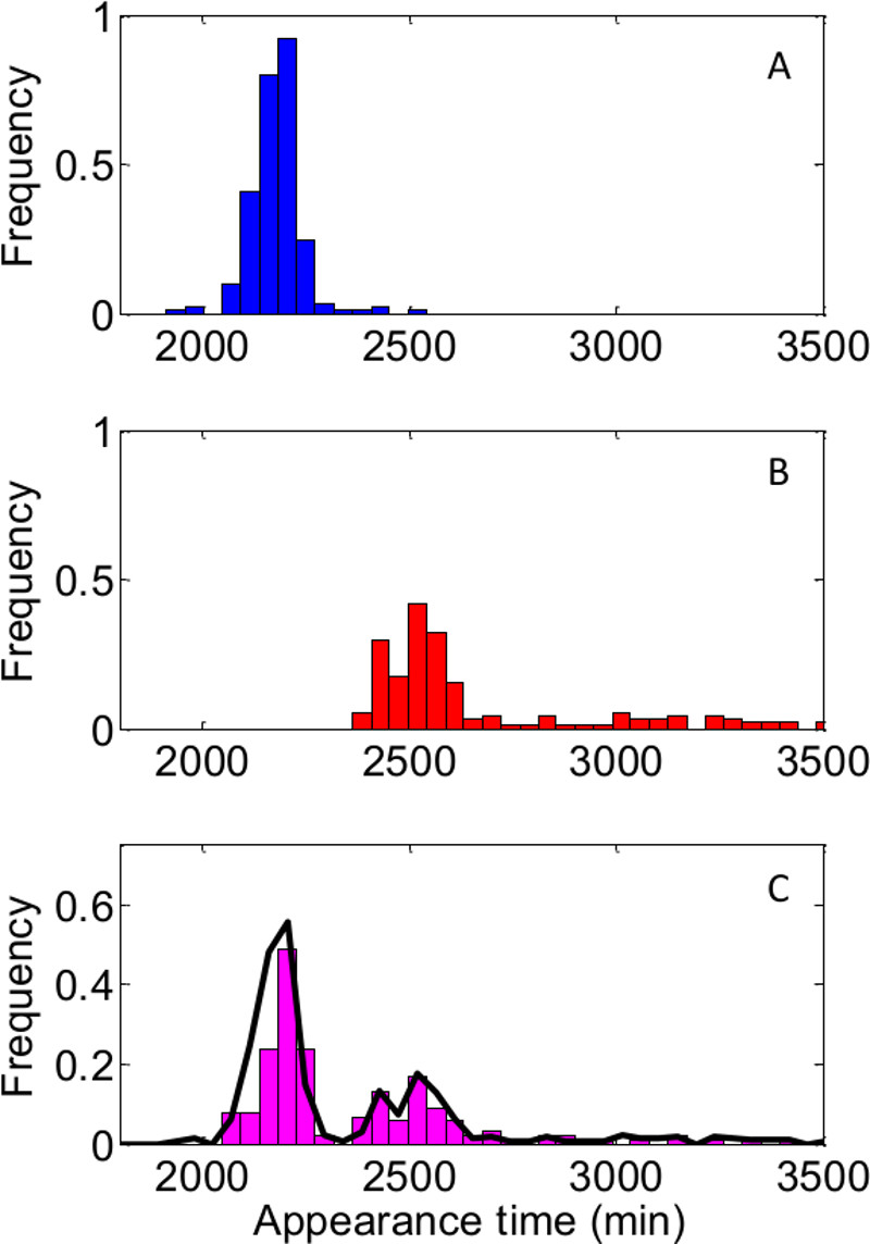
Figure 8. The appearance of early colonies does not interfere with the appearance of later colonies. (A) lag time distribution of wild‐type cells plated alone. (B) lag time distribution of a cold sensitive strain alone, after transfer to permissive temperature. (C) lag time distribution of both strains plated together under the same conditions. The black line represents the expected distribution based on the data obtained when measuring each strain separately. A good agreement between expected and measured distributions is obtained as long as the total number of colonies per plate is below 200.

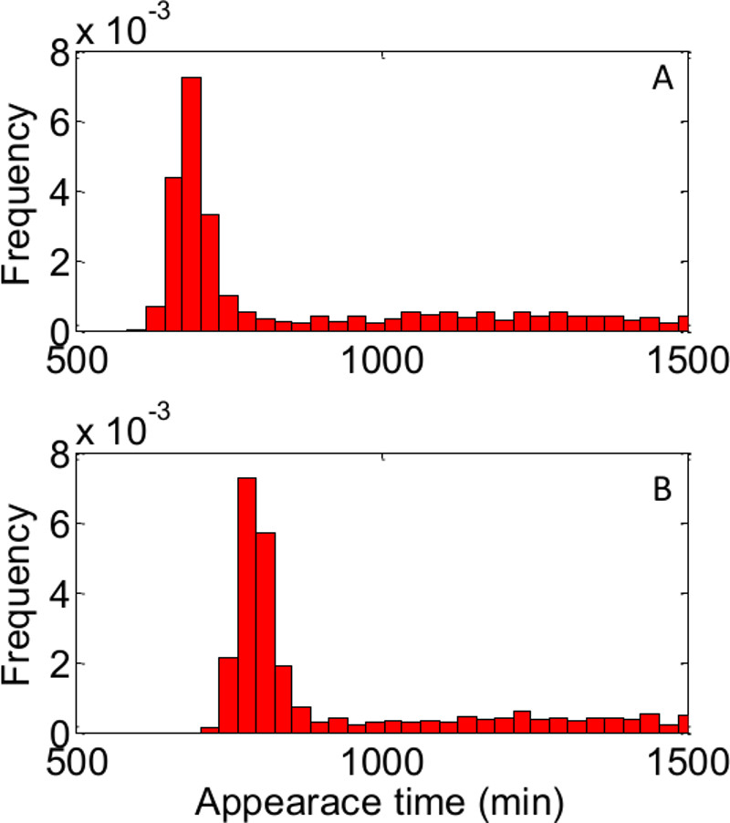
Figure 9. The detection threshold does not affect the shape of the colony appearance distribution. The colony appearance distribution was analyzed for the same data set using two different threshold sizes; (A) threshold size is 10 pixels; (B) threshold size is 50 pixels. Number of cells per histogram: approx. 1,500. The different detection threshold results only in a shift of the detection time.

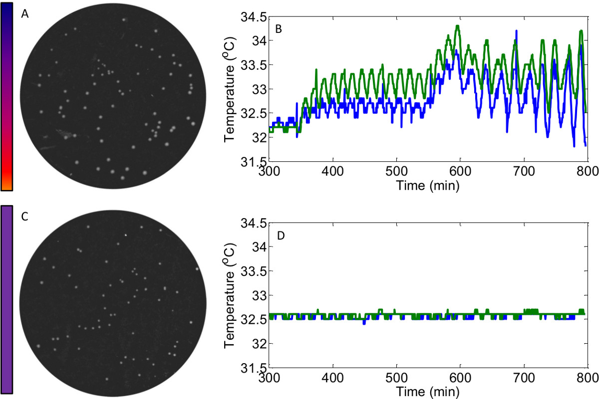
Figure 10. Temperature stability measurements across the scanner’s surface. (A) Image of a plate with colonies of Bacillus subtillis grown on the scanner without Power Management. The surface is warmer on the bottom and therefore the colonies grow faster. The gradual line beside the plate is a schematic representation of the heat gradient. (B) The temperature stability was measured with two thermocouples placed across the scanner’s surface. The scanner heats up during each scan and over the time. (C) With Power Management, the temperature is uniform and the colonies grow at similar rates. (D) Same as (B) with the Power Management module. Temperature stability of ±0.2 °C.

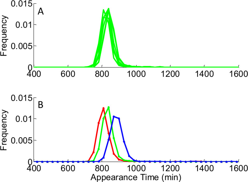
Figure 11. Differences in the appearance distribution may be due to differences in the volumes of solid medium. The same bacterial culture was plated on plates with different volumes of LB agar, resulting in a different height of agar surface. The different heights led to different opacity of the plates, and therefore a different detection time. The inter plates difference was checked and the difference between different height conditions. (A) Typical differences between plates of equal volumes of 30±0.5 ml of LB Agar. (B) Difference between different height conditions: the appearance distribution was measured for plates with volumes of 20±0.5 ml (red), of 30±0.5 ml (green) and of 40±0.5 ml (blue). Each condition is the average of 6 different plates. As long as the volume of the plates is within ±5 ml range, the opacity is similar and leads to similar appearance time distribution.

Discussion

Microscopic methods based on direct observation are often regarded as the “golden standard” for studying single-cell behavior. ScanLag, which enables measurement of the distribution of lag times in bacterial populations, provides data in good agreement with the distribution obtained from single-cell analysis and achieves much higher statistics.

Several critical steps have to be performed for this method to work well: first, do not compromise on the scanner resolution, which should be 4,800 x 9,600 to gain good images. Second, be aware that without the power management module (step 1.6), temperature gradient may develop on the flatbed surface and affect growth. Another important step is the filtration of defects such as dust that may have been mistakenly counted as colonies by the software. The built-in background subtraction of the software usually overcomes these defects, but sometimes “false” colonies have to be manually filtered.

The main troubleshooting steps might address inter-plate variation in the setup, due to several reasons: (a) The growth rate of microorganisms is affected by temperature. Different temperature and humidity conditions can occur due to uneven ventilation or location of the dish in the incubator. (b) The electronics of the scanner might heat up and cause a temperature gradient across the surface of the scanner. Figure 10 shows the influence of such spatial heat gradient on Bacillus bacteria, together with the measurements of the temperature on the scanner surface before and after implementing the power management module (step 1.6). Note that this module might not be necessary for newer scanners, and if only part of the scanner surface is used, power management may be unnecessary. (c) Plates with different opacity of the agar nutrient might lead to different levels of detection. Figure 11 shows the tolerance for different volumes of nutrient agar that result in different opacities.

Experimentally the ScanLag technique is easy to perform and requires only to plate microorganisms on standard Petri dishes, and to place them on the scanner’s surface. The software that was developed controls the entire procedure. The image acquisition is done automatically, and the image analysis for colony tracking is also automatic. Furthermore, the system can be scaled-up to measure many different conditions at the same time. Finally, the method relies on commercial office scanners and, therefore, is low cost.

This technique can be extended to the study of microorganisms which differ from E. coli K-12, however several considerations have to be made. First, the influence of early appearing colonies on the later ones has to be assessed, as described in detail in a previous publication⁷. For E. Coli K-12, the maximal density of CFU per plate is 200. Other strains with different sizes of colonies, and other possible cross talk between colonies, might require a different density. Second, the analysis of the plates is calibrated to specific software based thresholds that might need to be modified, depending on the contrast between the solid medium and the colonies. The software can be extended also to extract other colony characteristics, beyond lag and growth rate. The software code is open and can be modified to extract colony shape, brightness, smoothness and color.

Because measurements are made on colonies that originate from single cells, the data reveal new phenotypes that cannot be measured by population-level measurements. The importance of the lag time distribution is revealed in the presence of antibiotics. Many antibiotics are known to be effective only against growing cells; therefore as long as cells remain in the lag phase and do not grow, they are protected from effects of those antibiotics²¹. When the numbers of survivor bacteria are evaluated at time intervals during antibiotic treatment^15,22,23, a subpopulation of bacteria, called persisters, is often revealed. In certain cases, immunity to antibiotic treatment originates from prolonged lag. Using this setup, this lag is revealed and often has a non-trivial distribution²⁴ (Figure 6). This method also enables the retrieval of rare mutants. For example, after plating a mutagenized population, mutants can be identified based on phenotype and isolated directly, without selection. The setup could also monitor cell-cell interactions by measuring the growth of colonies as a function of the density of nearby colonies and to quantify phenomena such as quorum sensing or the spread of swarming bacteria. Multidimensional information uncovered by future experiments using this method will lead to better characterization of microbial populations and to advances in medical and environmental research.

Materials

List of materials used in this article

Name	Company	Catalog Number	Comments
Bacto agar	BD	214010
Difco LB broth	BD	240230
Petri dish 90 mm	Miniplast	20090-01
Epson Perfection v37	Epson	B11B207201	Flatbed Scanner with Optical resolution: 4,800 dpi, Hardware Resolution: 4,800 x 9,600 dpi, color bit depth 48-bit.
Epson Perfection v200	Epson	B11B188011
Epson Perfection 3490	Epson	B11B177011
ADU200 USB Relay	ONTRAK
Pieces of sterile black felt cloth	Custom made		Approximatly 100 x 100 mm
White plate holders	Custom made		Surface size, with 6 x 99 mm diameter hole
Delerin rings the size of the Petri dish	Custom made		Inner diameter: 72 mm Outer diameter: 86 mm Top outer diameter: 90 mm

References

- Bochner, B. R. Global phenotypic characterization of bacteria. FEMS Microbiol Rev. 33, 191-205 (2009).
- Monod, J. The growth of bacterial cultures. Annual Reviews in Microbiology. 3, 371-394 (1949).
- Penfold, W. J. On the Nature of Bacterial Lag. J Hyg (Lond. 14, 215-241 (1914).
- Powell, E. O. Growth rate and generation time of bacteria, with special reference to continuous culture. J Gen Microbiol. 15, 492-511 (1956).
- Elfwing, A., LeMarc, Y., Baranyi, J., Ballagi, A. Observing growth and division of large numbers of individual bacteria by image analysis. Applied and Environmental Microbiology. 70, 675-678 (2004).
- Hertog, A., et al. Simplified automated image analysis for detection and phenotyping of Mycobacterium tuberculosis on porous supports by monitoring growing microcolonies. PloS one. 5, (2010).
- Levin-Reisman, I., et al. Automated imaging with ScanLag reveals previously undetectable bacterial growth phenotypes. Nature Methods. 7, (2010).
- Lewis, K. Persister cells. Annual review of microbiology. 64, 357-372 (2010).
- Metris, A., George, S. M., Baranyi, J. Use of optical density detection times to assess the effect of acetic acid on single-cell kinetics. Applied and Environmental Microbiology. 72, 6674-6679 (2006).
- Niven, G. W., Fuks, T., Morton, J. S., Rua, S. A. C. G., Mackey, B. M. A novel method for measuring lag times in division of individual bacterial cells using image analysis. Journal of Microbiological Methods. 65, 311-317 (2006).
- Niven, G. W., Morton, J. S., Fuks, T., Mackey, B. A. Influence of environmental stress on distributions of times to first division in Escherichia coli populations, as determined by digital-image analysis of individual cells. Applied and Environmental Microbiology. 74, 3757-3763 (2008).
- Pin, C., Baranyi, J. Single-cell and population lag times as a function of cell age. Applied and Environmental Microbiology. 74, 2534-2536 (2008).
- Guillier, L., Pardon, P., Augustin, J. C. Influence of stress on individual lag time distributions of Listeria monocytogenes. Applied and Environmental Microbiology. 71, 2940-2948 (2005).
- Metris, A., George, S. M., Peck, M. W., Baranyi, J. Distribution of turbidity detection times produced by single cell-generated bacterial populations. Journal of Microbiological Methods. 55, 821-827 (2003).
- Balaban, N. Q., Merrin, J., Chait, R., Kowalik, L., Leibler, S. Bacterial persistence as a phenotypic switch. Science. 305, 1622-1625 (2004).
- Glaser, D. A., Wattenburg, W. H. An automated system for the growth and analysis of large numbers of bacterial colonies using an environmental chamber and a computer-controlled flying-spot scanner. Ann N Y Acad Sci. 139, 243-257 (1966).
- Guillier, L., Pardon, P., Augustin, J. C. Automated image analysis of bacterial colony growth as a tool to study individual lag time distributions of immobilized cells. Journal of Microbiological Methods. 65, 324-334 (2006).
- Michel, J. B., Yeh, P. J., Chait, R., Moellering, R. C., Kishony, R. Drug interactions modulate the potential for evolution of resistance. Proceedings of the National Academy of Sciences of the United States of America. 105, 14918-14923 (2008).
- Ernebjerg, M., Kishony, R. Distinct Growth Strategies of Soil Bacteria as Revealed by Large-Scale Colony Tracking. Applied and Environmental Microbiology. 78, 1345-1352 (2012).
- Rotem, E., et al. Regulation of phenotypic variability by a threshold-based mechanism underlies bacterial persistence. Proceedings of the National Academy of Sciences of the United States of America. 107, 12541-12546 (2010).
- Bigger, J. The bactericidal action of penicillin on staphylococcus pyogenes. Irish Journal of Medical Science. 19, 585-595 (1944).
- Hofsteenge, N., van Nimwegen, E., Silander, O. K. Quantitative analysis of persister fractions suggests different mechanisms of formation among environmental isolates of E. coli. BMC Microbiol. 13, 25 (2013).
- Moyed, H. S., Bertrand, K. P. Hipa a Newly Recognized Gene of Escherichia-Coli K-12 That Affects Frequency of Persistence after Inhibition of Murein Synthesis. Journal of Bacteriology. 155, 768-775 (1983).
- Balaban, N. Q. Persistence: mechanisms for triggering and enhancing phenotypic variability. Current Opinion in Genetics & Development. 21, 768-775 (2011).
Reprints and Permissions