Simultaneous Long-term Recordings at Two Neuronal Processing Stages in Behaving Honeybees

Summary

Simultaneous extracellular long term recordings from two different brain neuropiles or two different anatomical tracts were established in honeybees. These recordings allow the investigation of temporal aspects of neuronal processing across different brain areas at the single neuron as well as at the ensemble level in a behaving animal.

Abstract

In both mammals and insects neuronal information is processed in different higher and lower order brain centers. These centers are coupled via convergent and divergent anatomical connections including feed forward and feedback wiring. Furthermore, information of the same origin is partially sent via parallel pathways to different and sometimes into the same brain areas. To understand the evolutionary benefits as well as the computational advantages of these wiring strategies and especially their temporal dependencies on each other, it is necessary to have simultaneous access to single neurons of different tracts or neuropiles in the same preparation at high temporal resolution. Here we concentrate on honeybees by demonstrating a unique extracellular long term access to record multi unit activity at two subsequent neuropiles¹, the antennal lobe (AL), the first olfactory processing stage and the mushroom body (MB), a higher order integration center involved in learning and memory formation, or two parallel neuronal tracts² connecting the AL with the MB. The latter was chosen as an example and will be described in full. In the supporting video the construction and permanent insertion of flexible multi channel wire electrodes is demonstrated. Pairwise differential amplification of the micro wire electrode channels drastically reduces the noise and verifies that the source of the signal is closely related to the position of the electrode tip. The mechanical flexibility of the used wire electrodes allows stable invasive long term recordings over many hours up to days, which is a clear advantage compared to conventional extra and intracellular in vivo recording techniques.

Introduction

Honeybees as well as most other insects heavily rely on olfaction. Amongst others they use olfactory cues for orientation, mating, communication with conspecifics, and foraging. Their well elaborated olfactory system contributes to a rich repertoire of learning behaviors related to floral odor stimuli. These behaviors can be easily studied under controlled laboratory conditions (for review see^3-5). Their “mini brains” (cp.⁶) with their relatively small numbers of neurons makes the honeybee a well suited model organism for studying olfactory coding and learning during monitoring of neural activity.

The olfactory system in insects as well as in mammals shows analogous organization to a great extent (for review see^7,8). In honeybees about 80,000 receptor neurons⁹ situated in sensillae along the antennae^10,11 translate the environmental odor stimulus into a neuronal signal. Axons from olfactory receptor neurons innervate the antennal lobe (AL), which has a glomerular organization comparable to the vertebrate olfactory bulb. The AL comprises about 164 glomeruli interconnected with each other by about 4,000 local interneurons (LN) (for review see¹²). Especially in the honeybee it has been shown recently that LNs provide patchy lateral connectivity and that different subpopulations possess elemental and configural olfactory coding properties^13,14 . The AL was shown to be subdivided into a ventral and a dorsal hemi lobe giving rise to the medial and the lateral antennal lobe tract (m- and l-ALT; formerly termed m- and l-APT for medial- and lateral antennal lobe protocerebral tract^15-17). Here a new tract terminology introduced by a recent effort for a unified nomenclature of the insect brain will be used¹⁸. Both ALTs (l- and m-ALT) combine either 410 (l-ALT) or 510 (m-ALT) uniglomerular projection neurons (PN), respectively^15,16,19. PNs of both tracts have recently been shown to code odors in parallel² (for review see^17,20), and both tracts synaptically form divergent connections with Kenyon Cells (KC), the mushroom body (MB) principal neurons. Each MB contains about 172,000 KCs^21-23. The MBs are known to be involved in stimulus integration, learning, and memory formation. The axo dendrites of KCs form the peduncle (the mushroom´s stem), which has two main output regions: the vertica  or alpha- lobe and the horizontal  or beta-lobe^22,24. The output of the MB converges to only about 400 extrinsic neurons (EN)²⁴. ENs responsible for olfactory information processing mostly innervate the ventral aspect of the vertical lobe²². Recently, it has been shown that ENs recorded at this area encode the odor reward association²⁵.

Temporal aspects within the olfactory system of insects as well as vertebrates have become an important and significant aspect as a potential coding principle^26-29. To be able to simultaneously record multiple neurons from different sites at high temporal resolution, we established double multi unit recording techniques using customized multi channel wire electrodes introduced to different target regions in the bee’s olfactory system. This approach enables us to analyze and compare temporal processing in the honeybee olfactory system at the level of single neurons and populations of neurons either between parallel olfactory pathways, the dual olfactory pathway² or between different subsequent neuropils¹. Recently with a similar experimental approach in the locust olfactory system³⁰ using a different configuration of electrodes were able to analyze spatiotemporal coding mechanism for background-invariant odor recognition³¹. Thus, the established dual recordings enable gathering spatial information about simultaneous neuronal activity profiles.

Compared to the broader spatial sampling obtained from calcium imaging this method allows recording from two spots only. However, the advantage compared to calcium imaging techniques is the high temporal precision of action potential recordings, which cannot be provided by either conventional CCD imaging or 2-photon imaging acquisition. The extracellular electrodes described here are permanently implanted and fixed relative to the brain and head capsule avoiding electrode drift. This is a clear advantage compared to the usage of sharp intracellular electrodes. Another advantage compared to intracellular recordings and calcium imaging is the extended neural observation time ranging from many hours up to days. This is an important prerequisite to investigate neural correlates of learning and memory formation. Additional benefits of multi unit recordings are further outlined in the discussion section.

In this methodological overview the manufacturing procedure of custom design wire electrodes will be shown, adapted from^32,33 and suited for long term multi unit recordings in the honeybee brain. Additionally, an example how these types of electrodes are permanently implanted at two different recording sites within the honeybee olfactory system to record simultaneously the l- and the m-ALT over long periods of time to allow many stimulation protocols is shown². For verification of the recording positions an example and protocol for staining and post recording visualization of the recording sites is provided.

Protocol

1. Electrode Building (Figure 1)

1. Production of an electrode adapter that fits the electrode interface board of commercial multi channel amplifier systems^1,2,25.
   1. Use a small Plexiglas plate glued to an 18 Pin connector base.
   2. Connect the base with 3 short pieces of insulated wire to 3 separate soldering lugs screwed onto the Plexiglas plate (Figure 1 A1-A3).
   3. Insert a groove into the Plexiglas plate in which a glass capillary can easily move and be held in place by a screw (Figure 1 B1).
   4. Extend the glass capillary about 5 mm using a minutien pin.
   5. Attach the micro electrode wires along the minutien pin and the glass capillary to guarantee stabilization and support.
2. Multi-channel micro wire production (adopted from Ryuichy Okada^32,33)
   1. Span 3 micro wires (polyurethane coated copper wire, 15 µm diameter) in a way that they are placed next to each other (Figure 1 B2).
   2. Use a 12 V soldering needle to spread a thin film of low melting dental wax (50 °C) partially along the wires to glue them together (electrode tip) (Figure 1 B3). Leave a few centimeters unglued (electrode end) as this section will be used later to connect the micro wires with the electrode adapter.
3. Connect the multi channel micro wire to the electrode adapter
   1. Remove the glass capillary from the holder and attach it with the minutien pin to the electrode tip. Bring it into a position parallel to the micro-electrode (Figure1 B3).
   2. Glue the electrode tip to the minutien pin using low melting dental wax and cut the micro electrode at the tip, protruding 2-3 cm from the minutien pin and at the electrode end (small arrows Figure 1 B3).
   3. Slip the capillary slightly back into the electrode adapter. Use the screw to fix it (Figure 1 B4).
   4. Solder the loose ends of the three wires to the soldering lugs using a soldering gun with a temperature of around 360 °C to ensure melting of the insulation (Figure 1 B4). After soldering, ensure that there is adequate electrical contact (~300 kOhm).
   5. Mount one of the electrodes (master) to the electrode interface board of the headstage and fix the other multi channel electrode (slave) on a separate adapter. Connect the channels of the slave to the master electrode (Figure 1 C1). Additionally, solder the reference as well as muscle electrodes to the master electrode base (Figure 1 C2).

2. Bee Preparation (Figure 2)

In these described experiments, the honeybee (Apis mellifera), which is an invertebrate animal and therefore does not require specific ethical permits for usage, is used.

1. Catch honeybee foragers (A. mellifera) at the hive entrance in the morning as shown by others^34,35.
2. Chill the bees on crushed ice till immobilization (5 to 10 min) and fix one in a standard Plexiglas holder or metal tube in a way that the head is exposed (Figure 2 A). For minimizing head movements use low-melting dental wax (~50 °C) and fix the head carefully to the holder around the basis of the compound eyes and the neck.
3. Use low melting wax to fixate the scapi of the antennae on the head capsule (Figure 2 B) without touching the flagellum. The flagellum of the antenna needs to be pointed forward. Ensure that the bee can freely move its proboscis.
4. Shave the head capsule to ensure an undisturbed view and access to the top of the head.
5. Feed the bee with a 30% sucrose solution until saturation to ensure sufficient moistening of brain tissue and good viability of the animal (Figure 2 C).
6. Make careful incisions vertically along the borders of the compound eyes and horizontally above the antennal bases as well as beneath the ocelli and remove the loosened piece of cuticle (Figure 2 D).
7. Carefully set aside hypopharyngeal glands and remove the trachea to ensure a clear view and access to the brain prior to electrode insertion (Figures 2E, 2F).

3. Electrode Insertion

In the example case illustrated in Figure  2, one electrode is positioned aiming at the l-ALT, the other one aiming on the m-ALT². Using particular landmarks, other target regions are possible as well, for example the AL and MB output regions¹.

1. Position the electrodes using micromanipulators at the region of interest (Figure 2G and 3A). To target the m-ALT place the electrode between the AL and medially from the vertical lobe of the MB. Ensure the insertion site being above the branching point of the mediolateral ALT PNs. Protrude the electrode into the brain with a depth of about 180 µm (Figure 2E). For l-ALT PN recording place the electrode below the lateral protocerebrum (the LH) in the middle of an imaginary line between the lateral side of vertical lobe and the middle of the AL. Insert the electrode with a depth of about 300 µm (Figure 2E)
2. Insert the reference (silver wire, about 25 µm diameter) into the ipsilateral compound eye through a small cut in the cuticle. Insert another silver wire into the muscle projection region below the lateral ocelli. NOTE: If necessary the learning behavior of the bee can be monitored with high temporal precision by recording the muscle M17, which is involved in the proboscis extension response (PER) of the bee³⁶ as described in²⁵.
3. To solidly anchor the electrodes within the brain and the head capsule, cover the entire space above the brain with two component silicon (Figure 2H), which will prevent the brain from drying out. NOTE: the recordings can last for hours up to days, and the bees can for example be recorded during a classical conditioning procedure (Figure 2H) or stimulated with a large panel of different odors.

4. Data Acquisition and Preprocessing

1. Use proper acquisition software that meets the following requirements: sampling rate of min 25 kHz; analogue^1,25 or digital² cross differentiation between the electrode channels; band pass filter from 300 Hz to 8,000 Hz to extract spike events.
2. Use available spike sorting software to extract single unit activity, for example template matching techniques as included in the Spike2 software (Figure 3).
3. For further analysis use the time stamps of the extracted units to compute single unit averaged odor responses (Figure 4) or to calculate population vectors for Principal Component Analysis (PCA) (Figure 5) using commercially available software. To further analyze single unit and population response latency please compare recent publications^1,2,25.

5. Visualization of Relative Electrode Position (Figure 4)

1. Dip the electrodes tips into a solution of either 5% Alexa hydrazide 568 or 5% Alexa hydrazide 488 which is dissolved in 0.5 M potassium chloride solution prior to the recording experiments.
2. Remove the electrodes and the covering silicon carefully after the experiments, rinse the brain with bee Ringer solution, remove glands and trachea and insert tiny crystals of tetramethylrhodamin dextran or insert a 5% solution solved in 1.0 M potassium acetate into the AL to label the ALTs anterogradely. Perform the following steps in darkness.
3. Allow the dye to be taken up and transported by the projection neurons along their axonal tracts (30-45 min) (Figure 4A), before washing the brain with bee Ringer solution three times for another 30-45 min.
4. Chill the bee on ice until immobilization and carefully remove the brain from the head capsule. Fixate the brain by rinsing it in a 0.1 M PBS solution containing 4% formaldehyde and keep it overnight at 4 °C.
5. Wait at least 12 hr before washing the brain two times in 0.1 M PBS (10 min each).
6. Wash the brain 3x for 20 min in 0.2% Triton X-100 diluted in 0.1 M PBS before dehydrating it in an ascending alcohol series (30%, 50%, 70%, 90%, 95%, 3x 100% ethanol, 20 min each step).
7. Embed the dehydrated brain in Methylsalicylate on a microscope slide and seal it with a cover slide.
8. Use a confocal laser scanning microscope and scan the brain as optical sections every 2-5 µm using a Harmonic Compound Plan Apochromat objective (10X 0.4 NA immersion). Excite the tissue using 568 nm wavelength for tetramethylrhodamin dextran and a wavelength of 488 nm for the electrode position.
9. Reconstruct the stained brain structures and electrode paths from the image stacks in 3D with reconstruction software (e.g. AMIRA or Fiji) (Figure 4).

Results

"The present protocol allows simultaneous recordings at two different processing stages within individual honeybees and additionally allows to test underlying mechanisms of learning and memory via e.g., PER conditioning within restrained honeybees." This is a prerequisite for analyzing temporal aspects of neuronal processing. The method is easily adaptable for different scientific approaches to unravel the neuronal network of the bee’s olfactory system. For example this method is used (i) to analyze temporal processing of PNs within the dual olfactory pathway of the honeybee, the l- and m-ALT PNs (Figure 5). In Figure 5A one example of an l-ALT PN simultaneously recorded with a PN of the m-ALT is given as ten trial average and illustrates their response strength and latency in respect to five different odor concentrations as color coded heat plot. In an average of seven bees with 11 l- and 13 m-ALT PNs (Figures 5B, 5C) illustrates that both the response strength as well as the response latency, to a certain extent, reflects odorant concentration. Thereby PNs in this example increase their response strength while with increasing odorant concentration their response latency declined (Figures 5B, 5C). This result is rather limited and only valid for the analyzed odorant, but is still consistent with recent computational models of the AL³⁷. Whether odor concentration coding in the bee’s AL underlies non linear computations or underlies other coding properties still needs to be analyzed in future. Furthermore the method can be used (ii) to compare temporal aspects in the population activity at two subsequent processing stages, the AL- and MB-output (Figure 6). Principal component analysis (PCA) illustrates that odor computation is prolonged and outlast the entire odor presentation at the PN level whereas in ENs only the odor on and off set were represented in the population activity (Figure 6). Thereby the EN population reached their maximal activity already at a time point when the PN activity is still developing (cp. Movie 1).

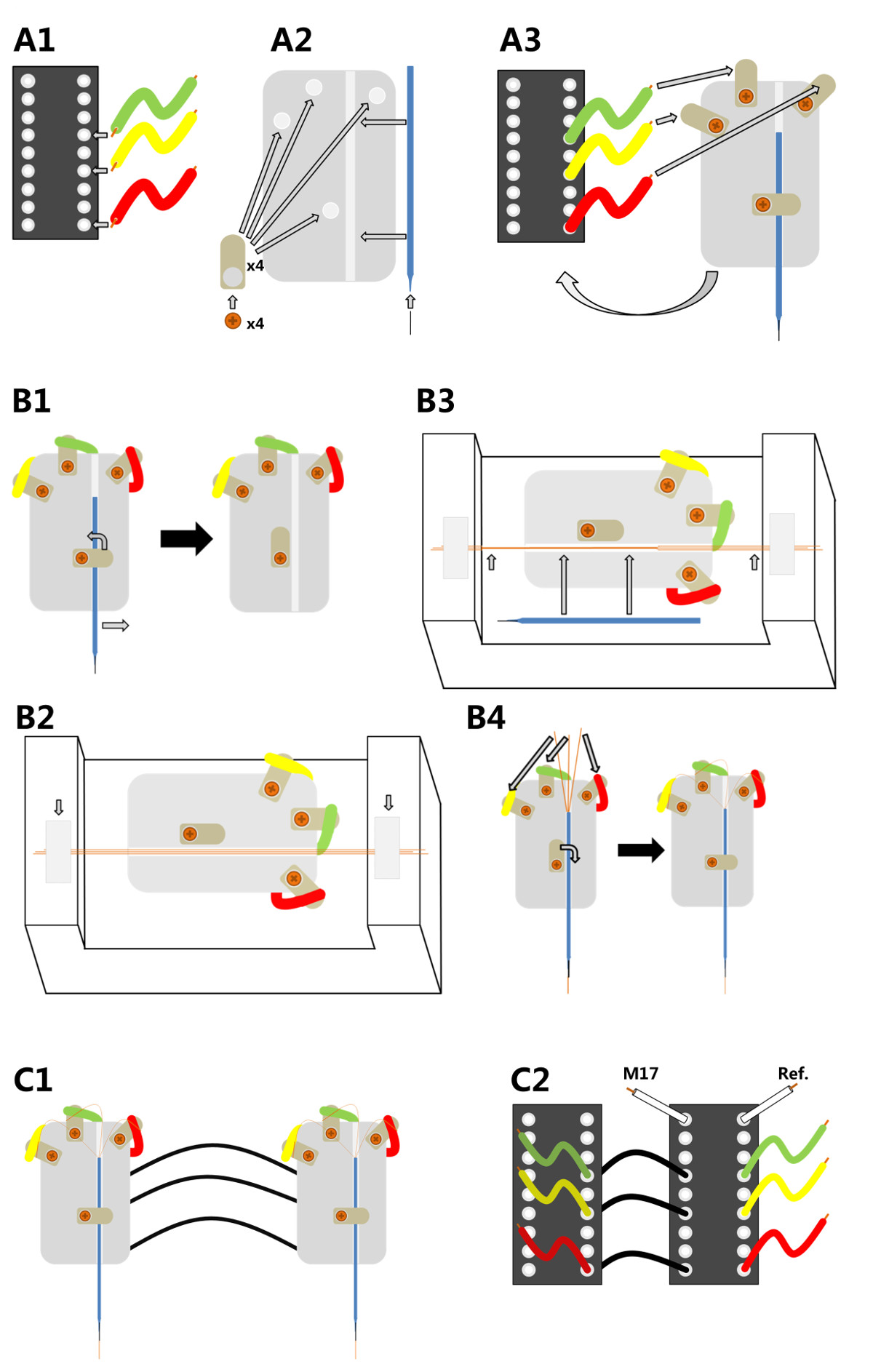
Figure 1. Manufacturing three-channel micro-wire electrodes. A1) The endings of three wires are soldered to an IC pin connector in Positions 11, 13 and 16. A2) Four soldering lugs are screwed onto a Plexiglas plastic base plate; a minutien pin is inserted into the tip of a glass capillary which is then attached to the plastic plate. A3) The plastic plate is glued on top of an IC pin connector and the free end of each wire is soldered to one of the top soldering lugs. B1) To equip the electrode holder with the fine copper wires, the capillary has to be taken out once more. B2) The base of the holder is then fixed in a custom made aligning device. Three copper micro wires are aligned along the groove and fixed with adhesive tape at each end. B3) The parallel micro wires are glued together with dental wax and the capillary is put back in place (long arrows); the glued micro wires are then attached to the capillary with dental wax and its ends are cut off (short arrows). B4) The three loose ends of the copper wires are soldered to the three top soldering lugs thus bringing them into electrical contact with the IC pin connector. C1) Two fully assembled electrodes can be connected to each other for use with a single headstage. C2) For this purpose the pins of one electrode (left, slave) are connected via insulated wires to the other electrode (right, master), which is connected to the head stage; the headstage connected electrode can also collect input from a muscle (M17) and reference electrode (Ref).

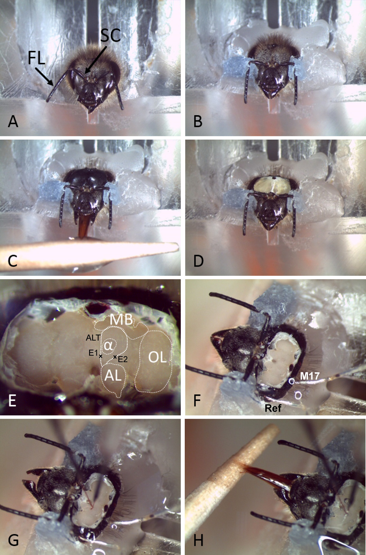
Figure 2. Preparation and permanent electrode insertion into the bee brain. A) A bee is inserted into a Plexiglas holder after immobilization on ice. Antennae with Flagellum (FL) and Scapus (SC) are indicated. B) The head and antennae are fixed using dental wax. C) The head capsule is shaved and the bee is fed with sugar water. D) The head capsule is opened. E) After removing glands and trachea from the top of the brain, the different neuropiles and major landmarks can easily be distinguished. The trajectories of the ALTs are indicated together with a mark where the electrodes are inserted. (MB: Mushroom body, AL: Antennal lobe, OL: Optical lobe, α: Alpha lobe or vertical lobe, ALT: antennal lobe tract, E1: electrode insertion side for m-ALT recordings, E2: electrode insertion side for l-ALT recordings). F) Reference (Ref) and muscle electrodes (M17) are inserted into the head capsule through little holes in the cuticle or the compound eye. G) The wire electrodes are inserted into the brain at the appropriate sites. H) After fixing the electrodes in place using two component silicon, the bee still shows PER and can be conditioned (e.g., using sugar water).

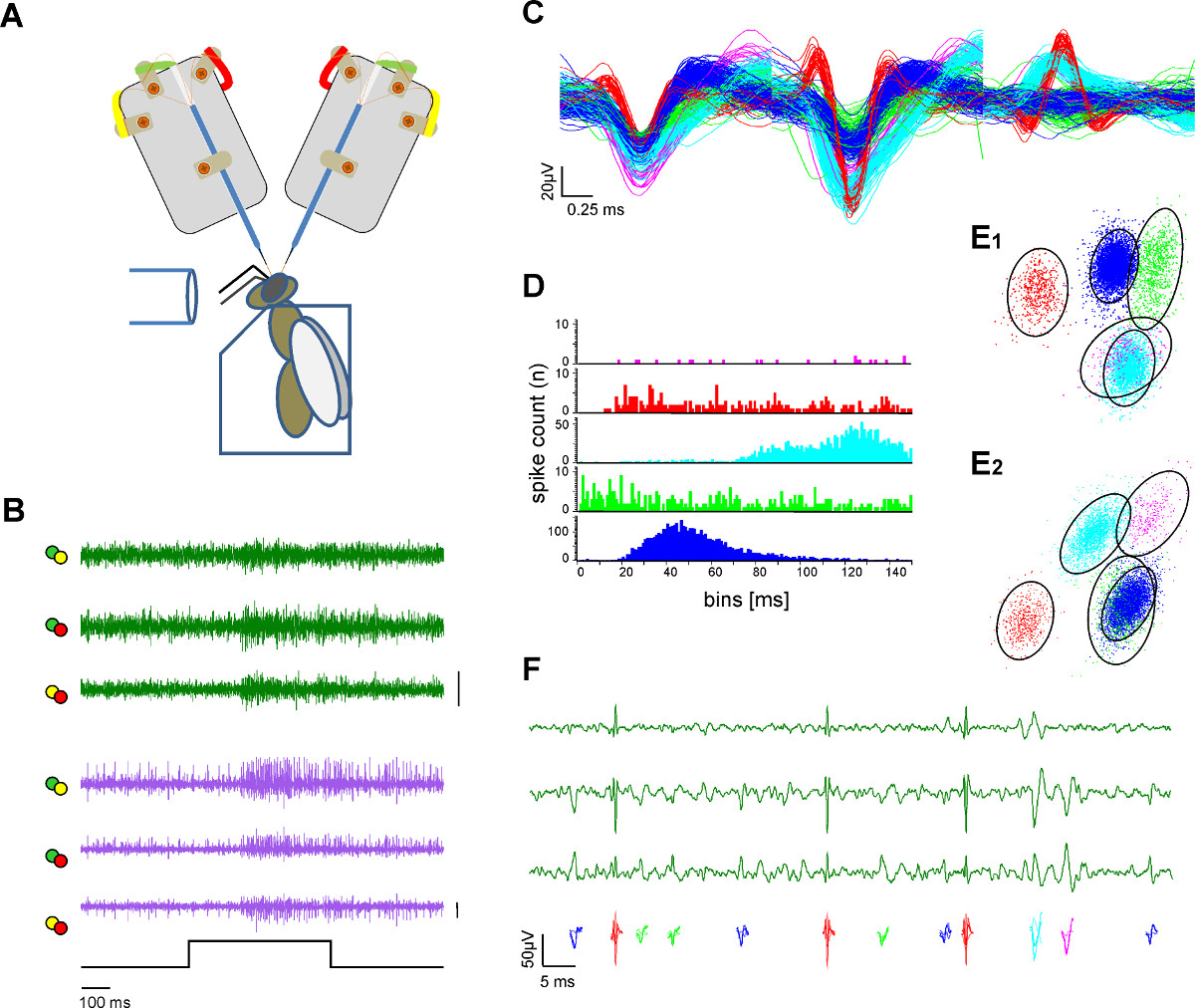
Figure 3. Extracellular recording at two neural tracts and single unit extraction (spike sorting). A) Schematic drawing of the experimental setup. The bee is fixated in a plexiglas holder. Odor stimulation is provided via a glass tube. Two electrode shanks are recording from the exposed bee brain. B) Simultaneous recordings from the l- and m-ALT PNs (green and purple traces) showing excitatory responses on both tracts to a 500 msec odor stimulation of honey in water solution at a concentration of 1:100 at 33 °C. Each plotted line represents the differentiated channels as color-coded label from the electrode soldering lugs in A. Bar: 50 µV. C) After spike sorting procedures single action potentials are sorted and color coded. Overlay of the sorted units illustrates the separation of the waveforms. D) Spike interval histogram indicates the separation quality of the sorted units as proof of adequate spike sorting. Note there is no spike within the unit’s refractory period. E) Two views (E1, E2) from a 3D clustering of the sorted unit with principal component analysis which indicates the distance of the sorted units to each other. Circles indicate the 2.5 fold Mahalanobis distance which resembles the SD in space and indicates a significant differentiation of the clusters in the principal component space F) Color coded units depict the action potentials visible in a magnification of three channels from one tract recording. Please click here to view a larger version of this figure.

Figure 4. Post-recording visualization and 3D-reconstruction of the recording position. A) Projection view of ortho-slices along the z-axes with maximum intensity alignment of an antero and retrograde backfilling of the uniglomerular projection neurons projecting from the AL to the MB and LH. The intracellular tracer Microruby (tetramethylrhodamin dextran) was inserted into the AL after the recording experiments. Stained glomeruli inside the AL proof proper PN staining. B) Projection view of ortho slices along the z -axes with maximum intensity alignment from a staining of the two electrodes with Alexa hydrazide 488 indicating the electrode placement for the m-ALT (E1, arrow) and l-ALT (E2, arrow). The tracer Alexa Hydrazide 488 migrates to the electrode surrounding tissue and stains the electrode insertion site. Note, the prominent staining in the AL is a superficial artefact. C) 3D Reconstructions of the stained target cells (PNs) and the electrode insertion site from A,B (right side) together with a schematic overview of the honeybee olfactory system (left side) with the indication of l- and m-ALT trajectories. Note, only uniglomerular PN tracts are shown. AN: antennal nerve, AL: antennal lobe, LH: lateral horn, MB: mushroom body, E1,E2: electrode insertion sites, m-ALT: medial antennal lobe tract, l-ALT: lateral antennal lobe tract, c: caudal, r: rostral, m: medial, l: lateral. Please click here to view a larger version of this figure.

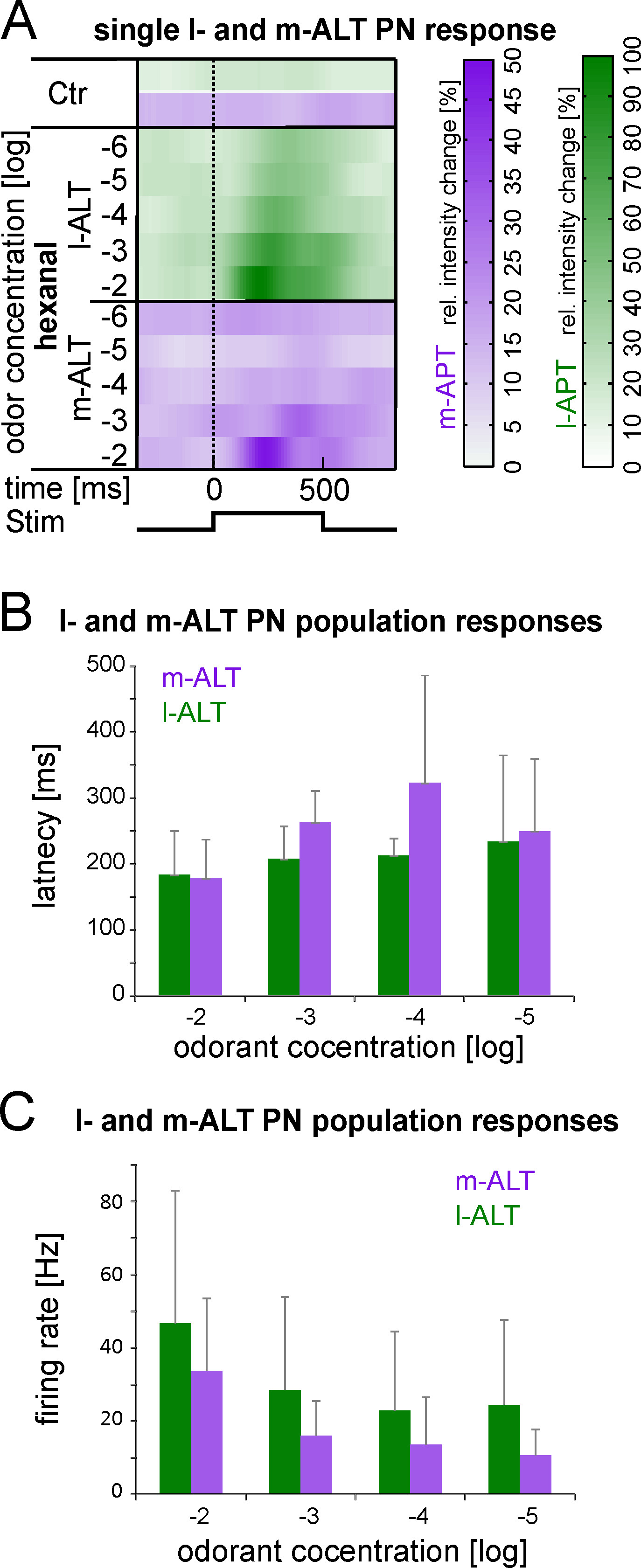
Figure 5. Example of odor concentration coding within the dual olfactory pathway. A) Heat plots illustrate the response of a single l-ALT (green) and single m-ALT PN (purple) acquired simultaneously from an individual honeybee in response to the odorant hexanal at increasing odor concentrations (from 1: 10^-6 to 1:100). Each line is an average of ten trial stimulation. The firing rate is shown as relative intensity change which is the firing rate in relation to the subtracted spontaneous activity. B) Population response latency of 11 l- and 13 m-ALT PNs from 7 recorded bees. In each bee the PNs from both tracts were recorded simultaneously. The population response latency shows a decreasing latency with increasing odor concentration in PNs from both tracts. The odor response onset at the antennae at 99 msec was recorded via electroantennograms and is subtracted from the PN response latencies. Note that at the lowest concentrations responses are too weak for latency measurements and, therefore, were excluded. C) Population response firing rate from same PNs as in B. With increasing odor concentration the response strength is increasing. The l-ALT shows a stronger response strength. In B,C the mean and SD are given.

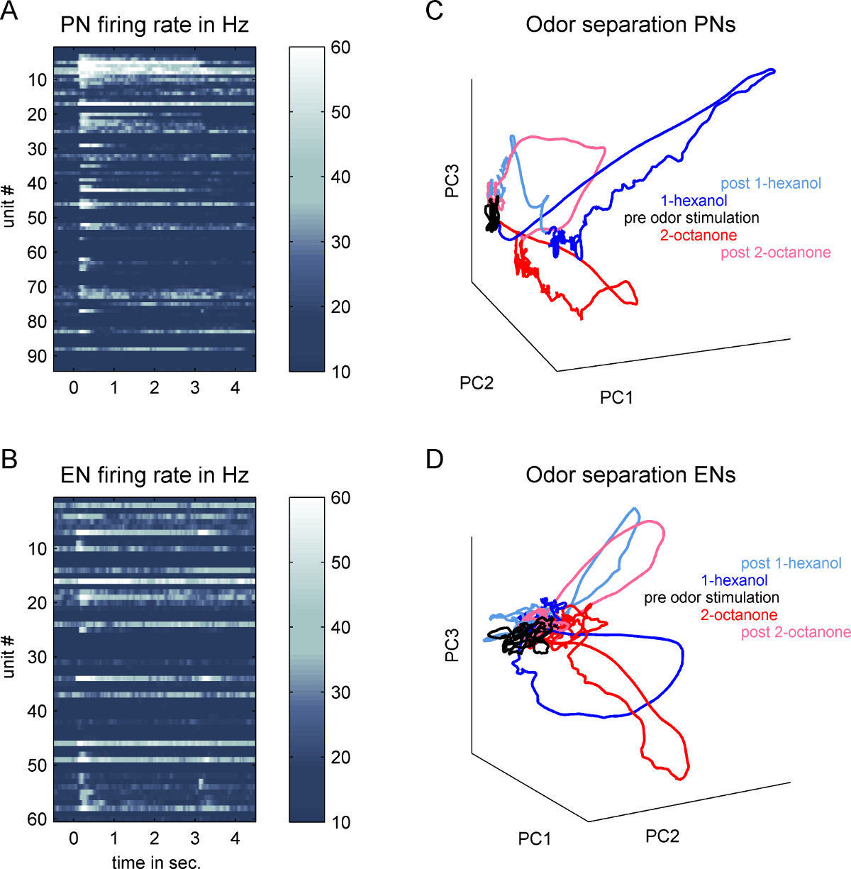
Figure 6. Comparing population activity at two subsequent processing stages along the honeybee’s olfactory pathway. Data were recorded in 20 animals which were stimulated with 1-hexanol and 2-octanone. A) Each line represents the false color coded mean firing rate of one projection neuron (PN) calculated across 10 odor repetitions of 1-hexanol. Odor presentation starts at time 0 and lasted three seconds. B) Shows the same as in A) but for mushroom body extrinsic neurons (EN). The matrix shown in A) can be seen as a PN population vector during odor stimulation with 1-hexanol. We calculated the same kind of population vector during odor stimulation with 2-octanone and used both vectors in a principal component analysis (PCA) keeping the temporal dimension. C) The first three principal components (PC1, 2 and 3) were plotted against each other to illustrate the odor separation in the PN ensemble activity at the antennal lobe output. The time before odor onset is marked in black. Activity during three seconds of stimulation with 1-hexanol is shown in blue. The activity during stimulation with 2-octanol is shown in red. Furthermore, we show 1.5 seconds (post) of the activity after odor of set of 1-hexanol (light-blue) and 2-octanonen (pink). Note that at the PN ensemble level, both odors evoking very distinct trajectories settle in a “fixed point” which outlasts the whole odor stimulation period. Only after odor offset the trajectories move back to the baseline activity without odor stimulation. D) The same analysis was done at the EN ensemble level representing the activity at the mushroom body output. Compared to the PN activity odors evoke a less distinct trajectory. Furthermore a “fixed point” is not observable. The initially odor induced trajectories intermingle with baseline activity although the odor is still present. Only the odor offset evoked an additional trajectory.

Movie 1. Time resolved evaluation of an odor induced trajectory after principal component analysis of a PN-population vector (left) and an EN population vector (right; cp. Figure 6). The upper parts include the first three principal components (PC1, 2 and 3) plotted against each other. The lower panels illustrate the evaluation of PC1, 2 and 3 over time. Odor stimulation is marked by the gray bar. All panels were synchronized. Note that the EN population activity starts slightly before the PN population activity, a phenomenon which seems to be contraintuitive but can be explained by the connectivity and properties of the involved layers, which is discussed earlier¹.

Discussion

This article demonstrates the production and usage of custom designed multi channel micro wire-electrodes. The described electrodes are suitable for recording both single unit and population activity which is especially useful for latency measurements and other temporal response properties of different neurons and different neuropils within a single specimen (for details see^1,2,25). Additionally we have shown how to permanently implement the micro wire electrodes to allow stable long-term recordings in behaving honeybees that last for hours up to days.

Extracellular multi-unit recordings became a favorable tool to achieve high temporal resolution combined with spatial information. In our case, these are either parallel neuronal tracts² or two different neuropils¹. Multiple neurons can be recorded and analyzed at the single neuron level in parallel and at high temporal resolution. Multi-unit recordings were first applied in mammals³⁸ and later also in insects^39-41. Substantial progress was achieved with the development and improvement of extracellular multi-channel recording techniques^42,43. This, for example, includes the development of new electrodes⁴⁴ or novel spike sorting and clustering algorithms⁴⁵. General methods of extracellular multi‐unit recording techniques are well described^46-48. The self built electrodes shown in this video additionally can be adapted by adding more microwires per electrode or the micro wires can be twisted to gain measureable constant distances between the tips. Both procedures would, however, lead to decreasing flexibility and increasing thickness of the electrode.

Compared to silicon probes commonly used for extracellular recordings in much larger insects like the hawk moth, locust and cockroach^40,49–51 the described micro wire-electrodes are smaller, flexible and can cope easily with potential brain movements and, thus, can be reliably used in small social insects like bees and ants that show a much broader behavioral repertoire. Most silicone probes have sharp shank like structures cutting axons and neural tissue along their insertion channel, while the described micro wires are round, flexible and smaller and are hence less harmful to the surrounding tissue which is a clear advantage if the goal is to study long-term plasticity in an intact and behaving animal. Another advantage of micro wire electrodes is their low cost production and the easy handling. Instead of carefully cleaning an expensive silicone probe the electrode wires are freshly cut prior to brain insertion and, therefore, lack problems of congestion. Furthermore it is possible to use more than one micro wire electrode in the same preparation either inserted in different neuropiles¹ or tracts² as we show here. This approach is especially favorable to analyze and compare temporal aspects like response latencies and interactions at different neural processing levels.

We are aware of the fact that an extracellular recorded signal does not reflect single cell activity per se. It is always a compound of voltage activity around the electrode tip. To pinpoint the source of the signal the difference of two neighboring micro wire channels within one electrode is always computed. Thus the source for the spike signals used to extract single unit activity were always very close to either one or the other electrode channel resulting in easily distinguishable spike waveforms. Signals from farther away, like muscle activity or activity of neighboring neuropils, reach both electrodes at the same time evoking comparable shapes and amplitudes and will be discarded by this procedure. Using the template matching technique of Spike2, we are very confident to obtain single unit activity, which is not the same, but very close to single neuron activity. However, the issue of spike sorting could be avoided by using intracellular recording techniques.

Single cell recordings with either sharp electrodes or patch pipettes allow indepth knowledge about physiological properties of a single neuron. However, due to the small size of insect neurons and their neurites (e.g., less than 1 µm for honeybee PNs ⁵²) only short term recordings are manageable. Furthermore, intra cellular recordings might be invasive and might harm the cell which is possibly another reason for the temporal limitations. In vivo intracellular recordings in insects rarely outlast one hour. A time window which was sufficient for the pioneering work of Martin Hammer⁵³ who recorded intracellular from a single identified neuron, the ventral unpaired maxilar neuron #1 (VUMmx1). He could link its activity directly to the reward pathway. Juliane Mauelshagen⁵⁴ registered intracellularly the activity of an identified mushroom body extrinsic neuron, the pedunculus extrinsic neuron#1 (PE1) during classical conditioning. The same neuron was in the focus of Menzel and Manz⁵⁵ when they found LTP after electrical stimulation of Kenyon Cells. However, Okada and colleagues⁵⁶ could use the intracellularly well characterized spiking pattern (double and triple spikes) for the identification of the PE1 during extracellular recordings. After all a combination of both methods, intracellular recordings from identified neurons and extracellular long term recordings might be a powerful tool for future investigations.

However, using sharp electrodes to record multiple cells (units) simultaneously at different processing levels over many hours up to days to analyze their temporal response relationships and/or even plastic changes is almost impossible.

With the first calcium imaging approaches in the honeybee^57,58 using calcium-sensitive dyes the analysis of spatial patterns of odor responses were accessible^59-62. However, in many cases the calcium sensitive dyes have to be introduced to the brain tissue via invasive manipulations that again limit the bee’s life span and intrinsic properties of the analyzed cells. This issue is overcome in other model organisms like the fruitfly using genetically introduced calcium sensors^63,64. However, in general, calcium sensors may introduce other limitations as they can act as calcium buffers that likely influence the temporal properties of odor responses. Simultaneous intracellular recordings combined with calcium imaging or computational approaches can prove the proper temporal resolution of imaging processes^65,66. However, the temporal resolution of the imaging process itself is rather limited. Optical acquisition systems usually use CCD-imaging with a temporal resolution of 5-20 Hz ⁶⁷, although 2-Photon-Imaging might be able to acquire faster sequences⁶⁸. However, increasing sampling rate always goes along with a loss in spatial resolution. Furthermore the calcium-sensitive dyes used in the honeybee undergo bleaching, which also reduces acquisition time⁶⁹.

Compared to other physiological recording techniques in insects our flexible multi-channel micro-wire electrodes ensure long-time access to single unit and population neuronal activity in behaving bees.

We demonstrated how to use two of these electrodes at different processing stages in the same animal, which facilitates the analysis of temporal coding aspects between the different recording sites. Dependent on the research problem and the model insect the basic method of electrode building demonstrated here is easily extendable and/or can be adapted. For example it is conceivable to use more than the three single wires to produce multi-channel electrodes. In addition, the number of recording sites can be extended and observing temporal aspects of more than two tracts or neuropils is feasible. Our hope is that this method will inspire many scientists and will contribute positively to the understanding of sophisticated neuronal processing in small brains.

Materials

List of materials used in this article

Name	Company	Catalog Number	Comments
Paraffin oil	Fluka	76235
Odors	Sigma Aldrich
PBS			pH 7.2
4% Formaldehyde	ThermoScientific	28908	Methanol free
Triton X	BioChemica	A1388
Methylsalicylate	Roth	4529.1
Tetramethylrhodamin dextran, 10,000 MW (Microruby)	Invitrogen	D7162	keep dark
Alexa 488 hydrazide	Invitrogen	A-10436	keep dark
Alexa 568 hydrazide	Invitrogen	A-10437	keep dark
Bee Ringer Solution	see Brill et al.2
Polyurethane-coated copper wire	Elektrisola	15 µm diameter & P155 insulation
Dental Wax	Densply Detrey	64103015S1	moderate melting point
Dental Wax	Flexaponal	124-202-00	low melting Wax
KWIK SIl	WPI	03L
18 Pin Socket	Conrad Electronic	189634-62
Hot melting glue	Conrad Electronic	827673
Soldering needle	Conrad Electronics	830283	12 V
Soldering terminal lug	Conrad Electronic	531901
Glaselectrodes	WPI	1B100F-3
Minutien Pins	Fine Science Tools	26002-20	V2A 0.2 x 12 mm
Switchable headstage	Tucer Davis Technologies	SH16
Headstage connection module	NPI	INT-03M
Amplifier Module	NPI	PDA-2F
Data Acquisition boards	National Instruments	NI-6123, Ni-6143
Acquisition Software	National Instruments	Lab View 8.2	custom design
Spike-Sorting	CED	Spike 2 v7.11
Matlab	Mathworks	R2008B
Micromanipulator	Leitz		manual
AG-wires	WPI	AGT05100
Confocal laser scanning microscope	Leica	TCS SP2 AOBS
AMIRA	Mercury Computer Systems	2/5/2000

References

- Strube-Bloss, M. F., Herrera-Valdez, M. a, Smith, B. H. Ensemble response in mushroom body output neurons of the honey bee outpaces spatiotemporal odor processing two synapses earlier in the antennal lobe. PLoS ONE. 7 (11), (2012).
- Brill, M. F., Rosenbaum, T., Reus, I., Kleineidam, C. J., Nawrot, M. P., Rössler, W. Parallel processing via a dual olfactory pathway in the honeybee. The Journal of neuroscience the official journal of the Society for Neuroscience. 33 (6), 2443-2456 (2013).
- Menzel, R. The honeybee as a model for understanding the basis of cognition. Nature Reviews Neuroscience. 13 (11), 758-768 (2012).
- Sandoz, J. Behavioral and neurophysiological study of olfactory perception and learning in honeybees. Frontiers in Systems Neuroscience. 5, (2011).
- Giurfa, M. Cognition with few neurons: higher-order learning in insects. Trends in Neurosciences. 36 (5), 1-10 (2013).
- Menzel, R., Giurfa, M. Cognitive architecture of a mini-brain: the honeybee. Trends in cognitive sciences. 5 (2), 62-71 (2001).
- Hildebrand, J. G., Shepherd, G. M. Mechanisms of olfactory discrimination: converging evidence for common principles across phyla. Annual Review of Neuroscience. 20, 595-631 (1997).
- Wilson, R. I., Mainen, Z. F. Early events in olfactory processing. Annu. Rev. Neurosci. 29, 163-201 (2006).
- Streinzer, M., Kelber, C., Pfabigan, S., Kleineidam, C. J., Spaethe, J. Sexual dimorphism in the olfactory system of a solitary and a eusocial bee species. The Journal of comparative neurology. 521 (12), (2013).
- Nishino, H., Nishikawa, M., Mizunami, M., Yokohari, F. Functional and topographic segregation of glomeruli revealed by local staining of antennal sensory neurons in the honeybee Apis mellifera. The Journal of comparative neurology. 515 (2), 161-180 (2009).
- Schneider, D. Elektrophysiologische Untersuchungen von Chemo- und Mechanorezeptoren der Antenne des Seidenspinners Bombyx mori L. Zeitschrift für Vergleichende Physiologie. 40 (1), 8-41 (1957).
- Menzel, R., Rybak, J. Antennal lobe of the honeybee. Handbook of brain microcircuits. , 427-432 (2011).
- Girardin, C. C., Kreissl, S., Galizia, C. G. Inhibitory connections in the honeybee antennal lobe are spatially patchy. Journal of neurophysiology. 109 (2), 332-343 (2013).
- Meyer, A., Galizia, C. G. Elemental and configural olfactory coding by antennal lobe neurons of the honeybee (Apis mellifera). Journal of comparative physiology. A, Neuroethology, sensory, neural, and behavioral. 198 (2), 159-171 (2012).
- Abel, R., Rybak, J., Menzel, R. Structure and response patterns of olfactory interneurons in the honeybee, Apis mellifera. The Journal of comparative neurology. 437 (3), 363-383 (2001).
- Kirschner, S., Kleineidam, C. J., Zube, C., Rybak, J., Grünewald, B., Rössler, W. Dual olfactory pathway in the honeybee, Apis mellifera. The Journal of comparative neurology. 499 (6), 933-952 (2006).
- Galizia, C. G., Rössler, W. Parallel olfactory systems in insects: anatomy and function. Annual review of entomology. 55 (August), 399-420 Forthcoming.
- Ito, K., Shinomiya, K., et al. A coordinated nomenclature system for the insect brain. Neuron. 81 (4), 755-765 (2014).
- Rybak, J. The digital honey bee brain atlas. Honeybee Neurobiology and Behavior. , 125-140 (2012).
- Rössler, W., Brill, M. F. Parallel processing in the honeybee olfactory pathway: structure, function, and evolution. Journal of comparative physiology. A, Neuroethology, sensory, neural, and behavioral. 199 (11), (2013).
- Mobbs, P. The brain of the honeybee Apis mellifera. I. The connections and spatial organization of the mushroom bodies. Philosophical transactions of the Royal Society of London. Series B, Biological. 298 (1091), 309-354 (1982).
- Strausfeld, N. J. Organization of the honey bee mushroom body: representation of the calyx within the vertical and gamma lobes. The Journal of comparative neurology. 450 (1), 4-33 (2002).
- Witthöft, W. Absolute Anzahl und Verteilung der Zellen im Hirn der Honigbiene. Zeitschrift für Morphologie der Tiere. 61 (1), 160-184 (1967).
- Rybak, J., Menzel, R. Anatomy of the mushroom bodies in the honey bee brain: the neuronal connections of the alpha-lobe. The Journal of Comparative Neurology. 465, 444-465 (1993).
- Strube-Bloss, M. F., Nawrot, M. P., Menzel, R. Mushroom body output neurons encode odor-reward associations. The Journal of neuroscience : the official journal of the Society for Neuroscience. (8), 3129-3140 (2011).
- Haddad, R., Lanjuin, A., Madisen, L., Zeng, H., Murthy, V. N., Uchida, N. Olfactory cortical neurons read out a relative time code in the olfactory bulb. Nature neuroscience. (May), 1-11 (2013).
- Martin, J. P., Beyerlein, A., et al. The neurobiology of insect olfaction: Sensory processing in a comparative context. Progress in neurobiology. 95 (3), 427-447 (2011).
- Nawrot, M. P. Dynamics of sensory processing in the dual olfactory pathway of the honeybee. Apidologie. 43 (3), 269-291 (2012).
- Farkhooi, F., Froese, A., Muller, E., Menzel, R., Nawrot, M. P. Cellular adaptation facilitates sparse and reliable coding in sensory pathways. PLoS computational biology. 9 (10), e1003251(2013).
- Saha, D., Leong, K., Katta, N., Raman, B. Multi-unit recording methods to characterize neural activity in the locust (Schistocerca americana) olfactory circuits. Journal of visualized experiments JoVE. (71), (2013).
- Saha, D., Leong, K., Li, C., Peterson, S., Siegel, G., Raman, B. A spatiotemporal coding mechanism for background-invariant odor recognition. Nature neuroscience. 16 (12), 1-13 (2013).
- Mizunami, M., Okada, R., Li, Y., Strausfeld, N. J. Mushroom Bodies of the Cockroach Activity and Identities of Neurons. Journal of Comparative Neurology. 519 (July), 501-519 (1998).
- Okada, R., Ikeda, J., Mizunami, M. Sensory responses and movement-related activities in extrinsic neurons of the cockroach mushroom bodies. Journal of Comparative Physiology A: Sensory, Neural, and Behavioral Physiology. 185 (2), 115-129 (1999).
- Haehnel, M., Froese, A., Menzel, R. In vivo Ca2+ imaging of mushroom body neurons during olfactory learning in the honey bee. Journal of visualized experiments JoVE. (30), (2009).
- Felsenberg, J., Gehring, K. B., Antemann, V., Eisenhardt, D. Behavioural pharmacology in classical conditioning of the proboscis extension response in honeybees (Apis mellifera). Journal of visualized experiments JoVE. (47), (2011).
- Rehder, V. Quantification of the honeybee’s proboscis reflex by electromyographic recordings. Journal of Insect Physiology. 33 (7), 501-507 (1987).
- Serrano, E., Nowotny, T., Levi, R., Smith, B. H., Huerta, R. Gain control network conditions in early sensory coding. PLoS computational biology. 9 (7), e1003133(2013).
- Hubel, D. H., Wiesel, T. N. Receptive fields and functional architecture of monkey striate cortex. The Journal of physiology. 195 (1), 215-243 (1968).
- Christensen, T. A., Pawlowski, V. M., Lei, H., Hildebrand, J. G. Multi-unit recordings reveal context-dependent modulation of synchrony in odor-specific neural ensembles. Nature neuroscience. 3 (9), 927-931 (2000).
- Byers, K. J. R. P., Sanders, E., Riffell, J. A. Identification of olfactory volatiles using gas chromatography-multi-unit recordings (GCMR) in the insect antennal lobe. Journal of visualized experiments JoVE. (72), e4381(2013).
- Perez-Orive, J., Mazor, O., Turner, G. C., Cassenaer, S., Wilson, R. I., Laurent, G. Oscillations and sparsening of odor representations in the mushroom body. Science. 297 (5580), 359-365 (2002).
- Stevenson, I. H., Kording, K. P. How advances in neural recording affect data analysis. Nature. 14 (2), 139-142 (2011).
- Buzsáki, G. Large-scale recording of neuronal ensembles. Nature neuroscience. 7 (5), 446-451 (2004).
- Viventi, J., Kim, D. -H., et al. Flexible, foldable, actively multiplexed, high-density electrode array for mapping brain activity in vivo. Nature neuroscience. 14 (12), 1599-1605 (2011).
- Pouzat, C., Mazor, O., Laurent, G. Using noise signature to optimize spike-sorting and to assess neuronal classification quality. Journal of neuroscience methods. 122 (1), 43-57 (2002).
- Lewicki, M. S. A review of methods for spike sorting: the detection and classification of neural action potentials. Network. 9 (4), R53-R78 (1998).
- Quian Quiroga, R., Panzeri, S. Extracting information from neuronal populations: information theory and decoding approaches). Nature reviews. Neuroscience. 10 (3), 173-185 (2009).
- Einevoll, G. T., Franke, F., Hagen, E., Pouzat, C., Harris, K. D. Towards reliable spike-train recordings from thousands of neurons with multielectrodes. Current opinion in neurobiology. 22 (1), 11-17 (2012).
- Riffell, J. a, Lei, H., Abrell, L., Hildebrand, J. G. Neural basis of a pollinator’s buffet: olfactory specialization and learning in Manduca sexta. Science. 164 (6), 877-892 (2013).
- Bender, J. a, Pollack, A. J., Ritzmann, R. E. Neural activity in the central complex of the insect brain is linked to locomotor changes. Current biology : CB. 20 (10), 921-926 (2010).
- Perez-Orive, J., Bazhenov, M., Laurent, G. Intrinsic and circuit properties favor coincidence detection for decoding oscillatory input. The Journal of neuroscience the official journal of the Society for Neuroscience. 24 (26), 6037-6047 (2004).
- Rybak, J. Die strukturelle Organisation der Pilzkörper und synaptische Konnektivität protocerebraler Interneuronen im Gehrin der Honigbiene, Apis mellifera.: eine licht- und elektronenmikroskopische Studie. , (1994).
- Hammer, M. An identified neuron mediates the unconditioned stimulus in associative olfactory learning in honeybees. Nature. 366, 59-63 (1993).
- Mauelshagen, J. Neural correlates of olfactory learning paradigms in an identified neuron in the honeybee brain. Journal of neurophysiology. 69, 609-625 (1993).
- Menzel, R., Manz, G. Neural plasticity of mushroom body-extrinsic neurons in the honeybee brain. The Journal of experimental biology. 208 (22), 4317-4332 (2005).
- Okada, R., Rybak, J., Manz, G., Menzel, R. Learning-related plasticity in PE1 and other mushroom body-extrinsic neurons in the honeybee brain). The Journal of neuroscience: the official journal of the Society for Neuroscience. 27 (43), 11736-11747 (2007).
- Joerges, J., Küttner, A., Galizia, C. G., Menzel, R. Representation of odours and odour mixtures visualized in the honeybee brain. Nature. 387, 285-288 (1997).
- Galizia, C. G., Joerges, J., Küttner, A., Faber, T., Menzel, R. A semi-in-vivo preparation for optical recording of the insect brain. Journal of neuroscience. 76 (1), 61-69 (1997).
- Galizia, C. G., Sachse, S., Rappert, A., Menzel, R. The glomerular code for odor representation is species specific in the honeybee Apis mellifera. Nature. 2 (5), 473-478 (1999).
- Sandoz, J. -C. Odour-evoked responses to queen pheromone components and to plant odours using optical imaging in the antennal lobe of the honey bee drone Apis mellifera L. The Journal of experimental biology. 209 (18), 3587-3598 (2006).
- Fernandez, P. C., Locatelli, F. F., Person-Rennell, N., Deleo, G., Smith, B. H. Associative conditioning tunes transient dynamics of early olfactory processing. The Journal of neuroscience the official journal of the Society for Neuroscience. 29 (33), 10191-10202 (2009).
- Locatelli, F. F., Fernandez, P. C., et al. Nonassociative plasticity alters competitive interactions among mixture components in early olfactory processing. European Journal of Neuroscience. 37 (1), (2013).
- Silbering, A. F., Bell, R., Galizia, C. G., Benton, R. Calcium imaging of odor-evoked responses in the Drosophila antennal lobe. Journal of visualized experiments JoVE. (61), 1-7 (2012).
- Strutz, A., Völler, T., Riemensperger, T., Fiala, A., Sachse, S. Calcium imaging of neural activity in the olfactory system of Drosophila. Genetically Encoded Functional Indicators. 72, 43-70 (2012).
- Galizia, C. G., Kimmerle, B. Physiological and morphological characterization of honeybee olfactory neurons combining electrophysiology, calcium imaging and confocal microscopy. Journal of Comparative Physiology A: Neuroethology, Sensory, Neural, and Behavioral Physiology. 190 (1), 21-38 (2004).
- Helmchen, F., Waters, J. Ca2+ imaging in the mammalian brain in vivo. European journal of pharmacology. 447 (2-3), 119-129 (2002).
- Stierle, J. S., Galizia, C. G., Szyszka, P. Millisecond stimulus onset-asynchrony enhances information about components in an odor mixture. Journal of Neuroscience. 33 (14), 6060-6069 (2013).
- Haase, A., Rigosi, E., et al. In-vivo two-photon imaging of the honey bee antennal lobe. Biomedical optics express. 2 (1), 131-138 (2010).
- Becker, P. L., Fay, F. S. Photobleaching of fura-2 and its effect on determination of calcium concentrations. The American journal of physiology. 253 (4 pt 1), C613-C618 (1987).
Reprints and Permissions