Measuring Respiratory Function in Mice Using Unrestrained Whole-body Plethysmography

Summary

The assessment of respiratory physiology has traditionally relied upon techniques, which require restraint or sedation of the animal. Unrestrained whole-body plethysmography, however, provides precise, non-invasive, quantitative analysis of respiratory physiology in animal models. In addition, the technique allows repeated respiratory assessment of mice allowing for longitudinal studies.

Abstract

Respiratory dysfunction is one of the leading causes of morbidity and mortality in the world and the rates of mortality continue to rise. Quantitative assessment of lung function in rodent models is an important tool in the development of future therapies. Commonly used techniques for assessing respiratory function including invasive plethysmography and forced oscillation. While these techniques provide valuable information, data collection can be fraught with artefacts and experimental variability due to the need for anesthesia and/or invasive instrumentation of the animal. In contrast, unrestrained whole-body plethysmography (UWBP) offers a precise, non-invasive, quantitative way by which to analyze respiratory parameters. This technique avoids the use of anesthesia and restraints, which is common to traditional plethysmography techniques. This video will demonstrate the UWBP procedure including the equipment set up, calibration and lung function recording. It will explain how to analyze the collected data, as well as identify experimental outliers and artefacts that results from animal movement. The respiratory parameters obtained using this technique include tidal volume, minute volume, inspiratory duty cycle, inspiratory flow rate and the ratio of inspiration time to expiration time. UWBP does not rely on specialized skills and is inexpensive to perform. A key feature of UWBP, and most appealing to potential users, is the ability to perform repeated measures of lung function on the same animal.

Introduction

Lung dysfunction is one of the leading causes of morbidity and mortality in the world. The condition is characterized by inadequate oxygen exchange, synonymous with coughing, chest pains and dyspnea. Respiratory disease accounts for ~10% of mortality worldwide¹. According to the World Health Organization, mortality rates are set to rise due to persistent smoking, pollution & occupational irritants. UWBP is a useful addition for studying lung physiology, which strongly compliments traditional biochemical and histological analyses². Other procedures used for lung assessment do not provide the same advantages as UWBP. Invasive plethysmography is a commonly used technique that requires the animal to be anesthetised^3,4 and thus, resulting respiratory measurements are not necessarily reflective of a natural state. Further, the requirement for mechanical ventilation and chemical challenges preclude future measurements^3,4. Another method of collecting respiratory data is by forced oscillation, which is more sensitive to finer changes in respiratory parameters compared to UWBP⁵. Forced oscillation is, however, an invasive technique and requires animal termination for data collection^5-7.

UWBP involves placing an animal inside a specialized chamber. During inspiration, the tidal air is warmed and humidified within the lungs increasing water vapor pressure and causes thermal expansion of gas⁸. This effect causes a net change in air volume creating an increase in pressure within the plethysmograph chamber⁸. The opposite occurs during expiration creating a respiratory waveform from the animal. Waveform analysis is then used to measure from the respiratory trace: respiration rate (breaths/min), total breathing cycle time (sec), inspiration/expiration time (Ti/ Te, sec) and changes in pressure due to each tidal volume (P_T). Figure 1 illustrates each measurements origin from a respiratory trace. These measurements are simple to calculate and multiple respiratory parameters may be derived from these measurements. These parameters include: Tidal volume (the volume of air moved between normal inhalation and exhalation), minute volume (volume of gas inhaled from the lungs per minute), inspiratory duty cycle (the percentage of inspiration time to the total breathing cycle duration) and inspiratory flow rate (the amount of air inspired in a given time).

UWBP provides precise, non-invasive, quantitative analysis of respiratory physiology in animal models and can be used for measuring the progression of respiratory disease and lung function^6,9. Contrary to other plethysmography techniques, UWBP avoids the use of anesthesia, restraints and invasive manipulations that produce artefacts and experimental variability^6,9. Anesthesia can suppress respiration, alter heart rate and can be challenging to regulate¹⁰. Restraints induce an increase in respiration due to additional stress via corticosterone and epinephrine release^11,13. The key feature of UWBP is repeated physiological assessment making it amenable to longitudinal studies. UWBP is strongly recommended for the longitudinal assessment of lung physiology and offers a valuable skill for future respiratory drug assessment.

Bleomycin, ovalbumin, and hypoxia have been utilized to induce respiratory challenges in several studies and UWBP has successfully measured accurate lung physiological assessment^7,9,13-16. The protocol described is designed for standard adult laboratory mice. However, UWBP has been adapted to other animals such as rats, guinea pigs, and non-human primates^17-20. UWBP is not restricted only to assessing pulmonary dysfunction but has also been used for the assessment of lung maturation³. The versatility, simplicity and reproducibility of UWBP have established an excellent technique for assessing pulmonary function in animals. Various software (see materials and equipment table) will be required to follow this procedure. An experienced scientist would be able to perform this protocol with a mouse within 1 hr.

Protocol

NOTE: The following experimental procedure is approved by the Animal Ethics Committee at Monash University and conducted in accordance with the Australian Code of Practice for the Care and Use of Animals for Scientific Purposes (2006). Adult female C57BL/6 mice used to generate the representative results were obtained from the Monash Animal Services. The mice were housed in a specific pathogen free, temperature and humidity controlled room with a 12 hr light-dark cycle. These mice had free access to food and water.

1. Initial Setup

1. Connect the laptop/desktop to the data acquisition machine for recording via a USB cable.
2. Connect the Bridge Amplifier from ‘output 1’ to ‘input 1’ of the data acquisition machine via a BNC cable.
3. Insert the pressure transducer into ‘channel 1’ of the Octal Bridge Amp. Turn the data acquisition machine on and open the analysis software. The software should automatically detect the equipment setup (see materials and equipment table).
4. Open Channel settings found in the setup tool bar of the software. Change the number of channels being recorded to 1.
5. Set up the barometer to measure room pressure and the water column apparatus to calibrate the Bridge Amplifier. The water column apparatus includes two 5 ml serological syringe pipettes connected by plastic tubing.
6. Fill the columns with water and ensure the water levels are balanced with a ruler. Connect one piece of plastic tubing to the top of each pipette. Figure 2 shows the water column set up.

2. Bridge Amplifier Calibration

Note: To calibrate the bridge amplifier an injection of air into the water column is required to create a 1 cm H₂O deflection. This will occur under a single set of conditions and is dependent upon the user's apparatus. For clarification these steps demonstrate how this laboratory would perform the calibration.

1. Withdraw a 1 ml syringe to 300 μl; attach the syringe to the stopcock at the end of the tubing on the right hand side of the water column. NOTE: Ensure that the stopcock is open to the syringe and the water column, and closed to the room air. If the water levels are not balanced at this point, turn the stopcock so that it is open to room air and the water column, this will rebalance the water. The tubing on the left hand side of the water column should be connected to the pressure transducer to measure the change in pressure induced by plunging the syringe.
2. Attach the tubing from the water column on the left hand side to the connector on the pressure transducer (top ring of the transducer).
3. Select the scroll down menu found next to channel 1 at the main screen on the right hand side of the software and select “Bridge amp” (see materials and equipment table).
4. Enter the settings to 5 mV, 20 Hz low pass, tick the ‘invert’ box and click ‘zero’. Click ‘zero’ to set the trace at ~0 mV. Reduce the window size to 4:1 for easier viewing.
5. With everything set up, depress the 1 ml syringe, leaving it for 3 sec. This will show a sudden spike on the software because the pressure has changed. When the 300 μl is depressed the pressure will move the water in the water column by 1 cm. This known value will help calibrate the Bridge Amplifier.
   NOTE: The pressure increase in the chamber due to the 300 μl depression corresponds to the P_K value used for later calculations.
6. Select ‘input units’ found on the bottom left hand corner of the Bridge Amp window.
7. Highlight the “background trace” prior to the spike otherwise known as the ‘Zero Region’.
   1. Click the arrow next to ‘point 1’ and this will produce the background signal within the range of -0.002 mV-0.002 mV (the value will never be exactly at 0 mV).
   2. Type ‘0’ in the window adjacent to the background signal window.
8. Highlight the “ increased pressure region of graph” from when the syringe is depressed. Click the arrow next to point 2 and the value should be in range of 0.9-1.2 mV.
   1. Type ‘1’ in the window next to the “increased pressure” window. For a visual clarification on steps 2.7 and 2.8 refer to Figure 3. Values found outside the ranges specified may indicate damage to the Octal Bridge Amp.
9. Go to ‘define units’ found at the top right corner of the window and select “cmH₂O”. If this option is not available, it may be entered manually. Click ok.
10. Return to the ‘Bridge Amp’ menu (refer to 2.1). Select 1 mV and set amplifier to ‘zero’. This will complete calibration and the water column can safely be removed.

3. Recording Lung Function

1. Weigh the mouse (g). NOTE: One week prior to physiological assessment introduce the mouse to the plethysmography chamber environment. This will aid in acclimatization and reduce stress when carrying out this procedure at a later date. For an overall schematic demonstrating the UWBP setup, please refer to Figure 4.
2. Measure the body temperature with a rectal thermometer. Lubricate the thermometer with petroleum jelly prior to insertion. Record the temperature reading and clean the lubricant off with 80% (v/v) ethanol. If using very small animals such as neonatal mouse pups, the mean body temperature value may be determined with an infra-red thermometer instead.
3. Place the temperature/relative humidity probe on the one-hole end of the plethysmography chamber. Record the temperature, humidity and barometric pressure inside the plethysmography chamber prior to placing the mouse within.
4. Place the mouse in the plethysmography chamber, cover the open end slightly. This allows the mouse to acclimatize. Close the chamber.
5. With the temperature/humidity probe inserted in the side of the plethysmography chamber with one hole, now insert the transducer and syringe in the other side with the two holes.
6. Press ‘Start’ on the software program and record for approximately 15-45 sec. Record 5-10 sec of data where the animal is not moving. Movement will alter the animal’s basal respiratory physiology and provide poor results. Respiration should oscillate in a linear path on the program. These are useable data. Note: Urination or defecation can lead to an increase in the temperature and humidity inside the plethysmography chamber. This will obscure results during analysis. In the event of urination or defecation, stop recording immediately and clean the plethysmography chamber with 80% (v/v) ethanol. Refer to Figure 6 for a visual representation of suboptimal results, where data should be rejected.
7. After recording for 45 sec, press ‘Stop’ on the software (see materials and equipment table) program. Remove the mouse from the plethysmography chamber and immediately record the chamber temperature and humidity. Do not continually record for more than 45 sec as this may stress the animal.
8. Return the mouse to its cage, spray and wipe the chamber with 80% (v/v) ethanol.
9. Allow the chamber to dry and return to baseline temperature and humidity before proceeding on to the next mouse. Repeat steps 3.1 to 3.9 for subsequent animals. Note: If multiple animals are being studied, ensure that the chamber temperature and humidity return to near baseline values before each new animal is put in the chamber.

4. Plethysmography Analysis

Note: To calculate respiratory parameters such as tidal volume (V_T) and minute volume the following variables need to be measured: respiration rate (breaths/min), total breathing cycle time (sec), inspiration/expiration time (Ti/ Te, seconds) and change in pressure due to each tidal volume (P_T). Figure 1 illustrates the variables that can be measured from a trace. The following steps use a software (see materials and equipment table) to measure these variables. When analyzing, avoid regions of the trace containing sniffing or movement. For reproducible results, at least 5 seconds of good breathing trace is required. For an example of different breathing traces refer to Figure 5 and 6.

1. Open the screen to full screen, set view to 1:1 and select 5 sec of usable data. A representative snapshot of this is shown in Figure 5.
2. Open the mini data pad window found at the top of the program in the DataPad tab. Select channel 1 and select ‘cycle measurements’ in the left hand column and ‘average cyclic height’ in the right hand column.
   1. Select ‘Option’ and set the scale for minimum peak detection to 1 (msec). This will allow detection of every peak value and becomes extremely important when using small animals that produce small oscillations.
   2. Click ‘OK’. This will present ‘Pressure deflection due to each tidal volume’ (P_T) measurement.
3. In the mini data pad, select ‘cycle measurements’ followed by ‘event count’ and click ‘OK’. This will present the ‘frequency’ (f) measurement.
   1. Frequency needs to be converted to breaths/min. This is done by multiplying the value by 60 sec and dividing the answer by the overall time of recording (min).
4. In the mini data pad, select ‘cycle measurements’ followed by ‘period’ and click ‘Ok’. This will present the ‘total breathing cycle time’ (T_tot, sec) measurement.
5. The next steps are used to create a macroinstruction to generate peak inspiration and expiration time values. Ensure the cursor is directly over the maximum of the peak/trough and add a comment on 9 sequential peaks and troughs. Begin with the peak of the oscillation as shown in Figure 5.
6. Subsequently, select window: data pad and column 1. In the window that appears click ‘selection information’ in the left hand column, ‘duration’ in right hand column and click ‘OK’.
7. Select macro found at the top of program and then start recording. Now select commands: ‘Find’, ‘Go’, ‘Start of File’ and click ‘Find’.
8. Select commands: ‘Find’ and ‘Find comments’. Type the same phrase typed for the comment box in the ‘containing’ box provided. Choose the ‘Select to Previous Point’ tab and ‘Find’.
9. Select commands: ‘Add to data pad’. Next, select macro: macro commands and begin repeat. The repeat count window that appears should be set at 9.
10. Select command: ‘Find next’. Select command: ‘Add to data pad’. Finally select macro commands and end repeat.
    1. Now select the macro and stop the recording. Save and name the macro after the animal number. NOTE: Setting up the macro for each animal allows the macro to be used for longitudinal studies and saves time.
11. The macro can now be run to obtain the Inspiration (T_i) and Expiration (T_e) time between each comment. The data will appear under channel 1 of the datapad. Expiration and inspiration occurs consecutively and the data will appear in this order.
    1. The data need to be manually split into inspiration and expiration values. Average the four data values of each parameter to obtain the mean T_i and T_e.
12. Once the primary values have been derived the tidal volume (V_T, ml) can be calculated. To obtain the tidal volume the equation of Drorbaugh and Fenn⁸ is used:
    V_T (ml)₌ (P_T / P_K) x (V_K) x ((T_CORE(P_B - P_C)) / (T_CORE(P_B - P_C) - T_C(P_{B -} P_CORE)))
    
    Where
    V_T: Tidal Volume
    P_k: Pressure deflection due to each injection of 1 ml (Refer to step 2.5)
    T_core: Core temperature of each animal
    P_C: Water vapor pressure at chamber temperature X Relative humidity in chamber
    T_C: temperature in animal chamber
    P_core: Pressure at body temperature (water vapor pressure at body temperature x 1.0)
    P_t: Pressure deflection due to each tidal volume
    V_k: Volume injection for calibration
     P_B: Barometric pressure
     
13. Once the tidal volume has been calculated the following parameters can also be determined:
    • Minute Volume (ml/min) = V_T x f
    • Minute Volume (ml/min/kg) = (V_T x f) / Body weight (kg)
    • V_T (ml/kg) = V_T (ml) / Body weight (kg)
    • Inspiratory Duty Cycle (%) = T_i / T_tot
    • Inspiratory Flow Rate (ml/sec) = V_T / T_i
    • Ratio of inspiration time to expiration time = T_i / T_e
    • Total cycle time (sec) = Inspiration time (sec) + Expiration time (sec)

Results

When this procedure has been followed correctly, a consistent oscillating trace is created on the data analysis software. The procedure provides a respiratory trace within a few minutes after setup with simple computing calculations to determine respiratory parameters listed. Figure 5 represents a suitable breathing trace from a control (healthy) mouse. Appropriate oscillating data is produced when the animal is not actively moving.

UWBP is an extremely useful and reliable assessment of lung function between control and pulmonary fibrosis cohort. Figure 7 demonstrates the lung function of a mouse with bleomycin-induced pulmonary fibrosis at day 14. In comparison to the control graph, Figure 7 illustrates a visual difference consistent with bleomycin administration⁷. As discussed previously, the procedure may be repeated allowing us to observe changes in respiratory parameters over time between these two groups.

Results obtained are to be expressed as means ± SEM. It is recommended to copy and paste the data collected into a simple Excel spreadsheet. This will become useful for carrying out calculations discussed in steps 4.13 & 4.14. Respiratory function can be compared visually between two groups as demonstrated in Figure 8.

Figure 1. Different components of the breathing cycle illustrated using the barometric plethysmography. This graph illustrates a) the change in pressure due to inspiration (∆Pi), b) the change in pressure due to each tidal volume (PT), c) the change in pressure due to expiration (∆Pe), d) total breathing cycle time (Ttot), e) inspiration time (Ti) and f) expiration time (Te). Click here to view larger image.

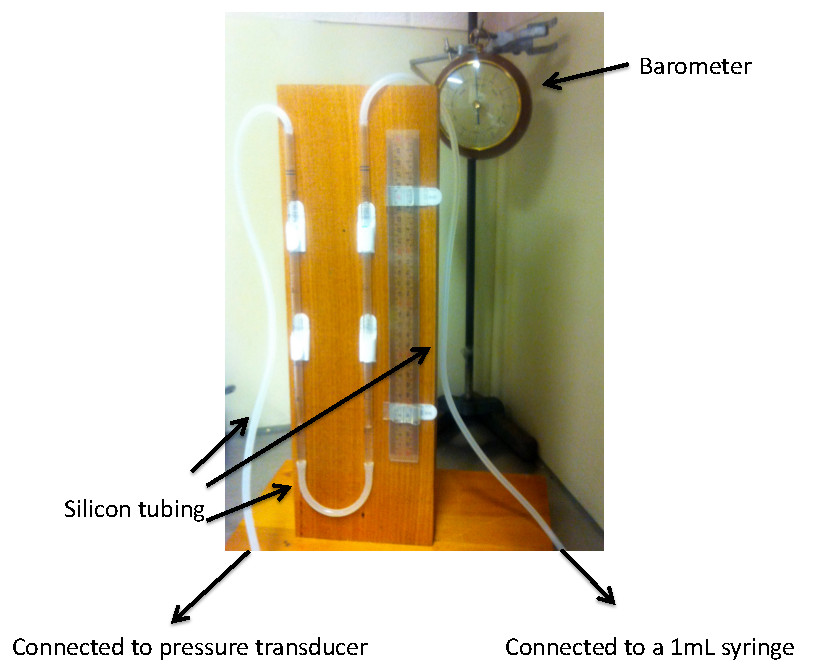
Figure 2. Visual representation of the barometer and water column setup. The figure is designed to aid the reader in setting up the barometer and water column for the calibration process. Notice the water is level within the two columns aided by the ruler. The two columns are connected via 15 cm of plastic tubing. The tubing on the right (65 cm) is connected to a 1 ml syringe and to the left (75 cm) the pressure transducer linked to the data acquisition machine. Note: the length of tubing determines the volume (300 μl) required to move 1 cm of water. Click here to view larger image.

Figure 3. Performing steps 2.4 and 2.5 of Bridge Amp Calibration. This figure illustrates the steps 2.7 and 2.8 for calibration of the equipment. It is crucial to correct the Bridge Amp to obtain precise results. Click here to view larger image.

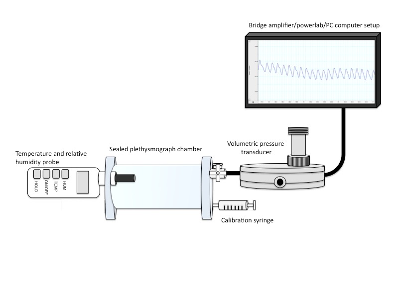
Figure 4. An overall schematic of the UWBP setup. To the left is the humidity/temperature probe connected to one side of the plethysmography chamber containing the animal. To the right is the calibration syringe and pressure transducer leading from the plethysmography chamber to the data acquisition system producing a respiratory trace on the computer. Click here to view larger image.

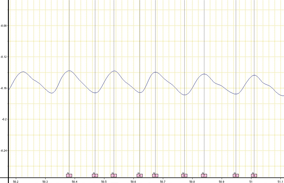
Figure 5. An example of a respiratory breathing trace from a C57Bl/6 control mouse obtained when using UWBP. This breathing trace illustrates appropriate, consistent data from a control animal. Nine consecutive comments are added at the peaks and troughs of breathing oscillations to obtain the respiratory parameters listed by following steps 4.1-4.13. Time is represented along the x-axis (sec) and pressure changes along the y-axis (cm.H₂O). Click here to view larger image.

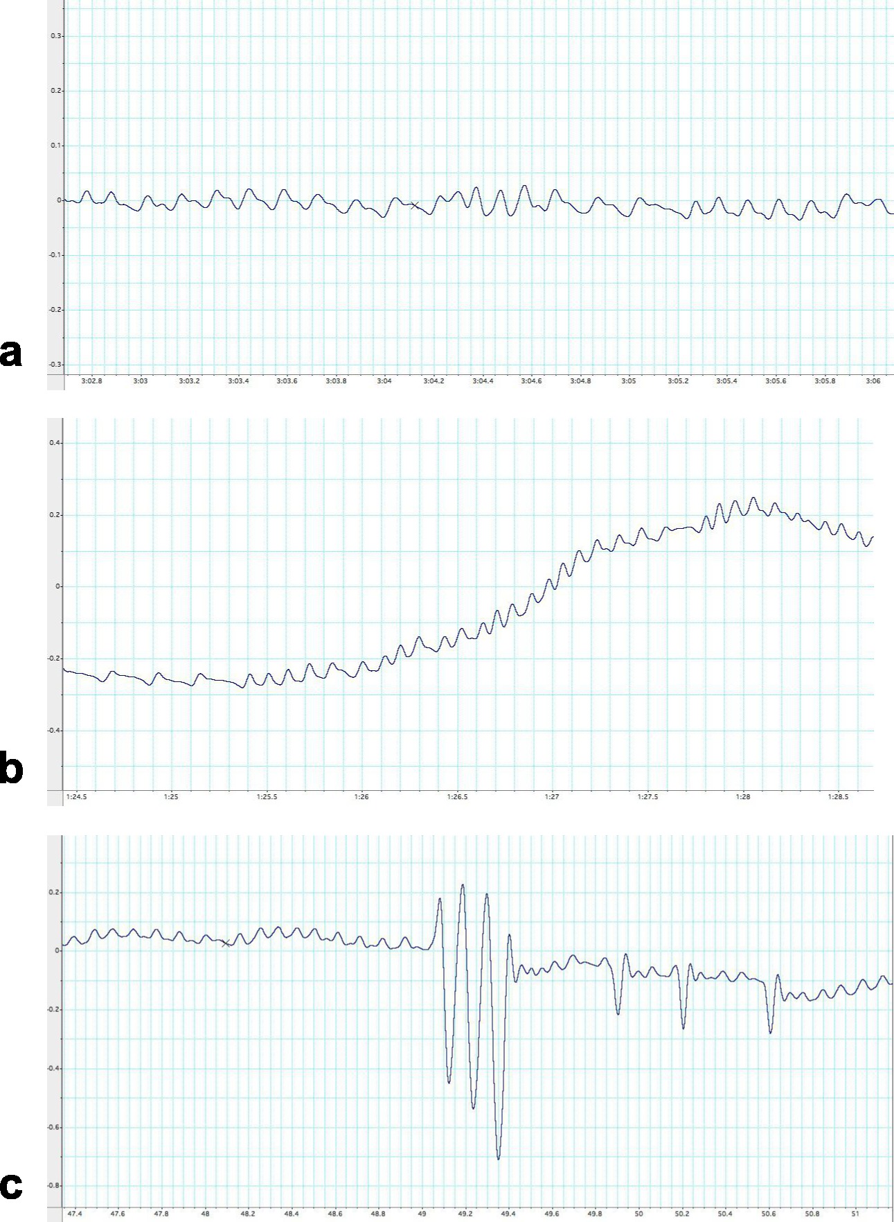
Figure 6. Examples of different suboptimal traces obtained from a C57Bl/6 mouse when using UWBP. Suboptimal results can be confused as appropriate data and is the most common source for poor analysis. This figure illustrates the most common suboptimal traces that should never be used for analysis. These breathing traces demonstrate a) A breathing trace recorded while the animal is sniffing and moving altering the animal’s basal respiratory physiology. b) A trace recorded resulting oscillations gradually increasing over time is usually caused by condensation and humidity build up. However, the trace may be corrected by wiping the plethysmography chamber with ethanol or by repeating the calibration steps. c) A trace recorded during plethysmography chamber movement while the animal or researcher is engaging with the equipment. Time is represented along the x-axis (sec) and pressure changes along the y-axis (cm.H₂O). Click here to view larger image.

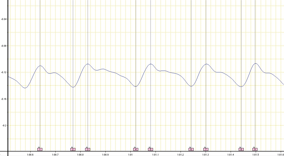
Figure 7. An example of a breathing trace obtained from a C57Bl/6 mouse with induced pulmonary fibrosis when using UWBP. This breathing trace illustrates appropriate, consistent data from an animal with induced pulmonary obtained when using the UWBP procedure described in this article. Nine consecutive comments are added at the peaks and troughs of breathing oscillations to obtain the respiratory parameters listed by following steps 4.1-4.13. Time is represented along the x-axis (sec) and pressure changes along the y-axis (cm.H₂O). Click here to view larger image.

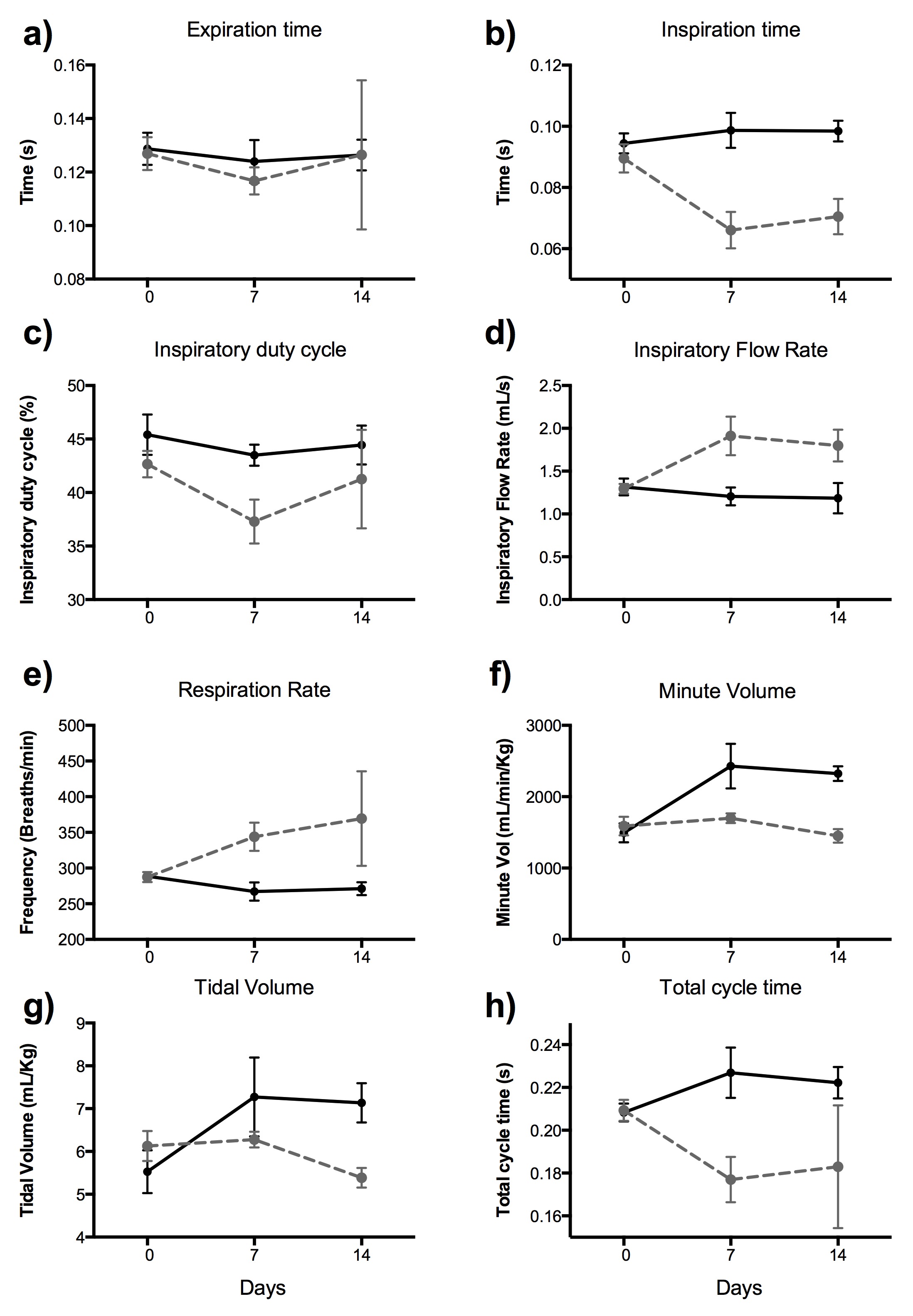
Figure 8. Respiratory function compared between control and bleomycin challenged C57Bl/6 mice. Performing plethysmography analysis after using UWBP will allow the user to results similar to what is represented here. This figure demonstrates the physiological differences between bleomycin challenged animal (dotted grey line) and control animals (solid black line). These graphs show comparisons in a) Expiration time (sec), b) Inspiration time (sec), c) Inspiration duty cycle (%), d) Inspiratory flow rate (ml/sec) e) Respiration rate (breaths/min), f) Minute volume (ml/min/kg), g) Tidal volume (ml/kg) and h) Total cycle time (sec). Lung function data were collected longitudinally in the same cohort of animals on days 0, 7, and 14 following bleomycin challenge. Representative data has been adapted from Murphy et al. (2012)¹⁶. Click here to view larger image.

Discussion

The technique described here is a non-invasive method for assessment of respiratory parameters of unrestrained and unanesthetized mice. The strengths of this protocol include its simplicity and precision to measure lung function longitudinally with minimal artefacts. There are, however, some limitations and critical steps to be noted about the procedure. Firstly and most importantly, the mouse must stay calm within the chamber for a minimum of five seconds. Added stress will disrupt the breathing pattern of the mouse and hence provide variable results (Figure 6a). This drawback will likely remain and is to be expected at times. However, replacing the mouse in its home-cage and allowing it time to resettle will easily correct this. It is crucial that the animal feels comfortable within the chamber environment to obtain five seconds of appropriate/useable data. Further consideration is required regarding the chamber environment. The environment, unrelated to respiratory mechanics, can significantly affect results. As the duration of assessment increases, the humidity and temperature of the chamber increases, as well as decreasing available oxygen, significantly impacting on ventilation. The timing of ventilation increases the humidity and temperature of the chamber as well as decreasing available oxygen²¹. A small leak in the chamber can aid in reducing thermal drifts created from heat production^22,23. The protocol discussed is specific to the equipment and instrumentation listed. Calibration of the bridge amplifier in section two will depend upon the reader’s equipment. If factors such as the tubing length are different a 300 µl injection of air may not cause a 1 cm.H₂O deflection.

There are also physiological differences depending on the time of analysis. Rodents are naturally nocturnal creatures and circadian cycles, which ultimately generate changes in respiration, should be taken into account when timing the experiments²⁴. It is thus necessary to time and plan the experiments such that experimental data can be accurately compared between cohorts. It is also important to take note of the trace movement. If the oscillations are not running in a linear pattern, it is usually due to a build up of condensation or humidity within the chamber (Figure 6b), or ineffective seal on the chamber. Ultimately, these limitations can be accounted for and the UWBP process performed appropriately to provide precise respiratory measurement. It is also important to note that this method will require modification (smaller chamber size) for measuring respiratory changes in neonatal standard laboratory mice (e.g., <2 weeks C57Bl/6) in order to detect pressure changes in the respiration of animals of that size.

Although UWBP demonstrates considerable advantages it also carries controversy. Investigators should familiarize themselves with the debate and make an informed decision whether this technique is appropriate for the research question. Initially, Drorbaugh and Fenn (1955)⁸ believed that an increase in the chamber pressure is caused by inspired air being warmed and humidified to pulmonary values; the opposite occurred in expiration. This allowed the calculation of tidal volume. Subsequent research considered that the pressure changes were caused by changing alveolar pressure during the generation of airflow²⁵. This work stated the use of plethysmography for airway resistance calculation. Enhorning et al. (1998)²⁶ provided evidence that tidal volume, respiratory rate and airway resistance all influence pressure fluctuations within the plethysmography chamber. When the air in the chamber is heated and humidified to body conditions pressure fluctuations are reduced by two-thirds and are amplified through increased resistances²¹. As all these components reflect pressure fluctuations there is controversy whether measurements of a particular respiratory parameters are accurate. As a result it has been concluded that tidal volume obtained from plethysmography is a qualitative rather than quantitative assessment²⁶. Both upper and lower airway resistances are components of the plethysmography system creating uncertainty in measuring bronchoconstriction²⁷. It is of the author’s opinion that UWBP should be used reciprocally with invasive analyses. It is, in fact, the policy of certain journals that manuscripts solely based upon UWBP data will not be accepted. This will be another consideration for the reader.

In summary, UWBP is a useful method to measure changes to respiratory parameters in standard laboratory rodents, particularly amenable to longitudinal studies. Key advantages of this technique are the avoidance of invasive procedures, chemical challenges and requirement of anesthesia. This allows the researchers to collect physiological data that most closely represent naturally occurring events and reduce experimental variability.

Materials

List of materials used in this article

Name	Company	Catalog Number	Comments
LabChart 7 software (for Macintosh)	ADINSTRUMENTS	MLU60/7	used in protocol step 4
PowerLab 8/30 (model ML870)	ADINSTRUMENTS	PL3508
Octal Bridge Amp (model ML228)	ADINSTRUMENTS	FE228
Black BNC to BNC cable (1 m)	ADINSTRUMENTS	MLAC01
Macintosh OS	Apple Inc.		Mac OS X 10.4 or later
Surgipack Digital Rectal Thermometer	Vega Technologies	MT-918
Grass volumeteric pressure transducer PT5A	Grass Instruments Co.	Model number PT5A; serial No. L302P4.
1 ml Syringe	Becton Dickinson (BD)	309628
5 ml Serological syringe pipettes	Greiner Bio One	606160	Connected via plastic tubing
Balance/Scales	VWR International, Pty Ltd	SHIMAUW220D	Any weighing balance with of 0.1 gram resolution
HM40 Humidity & temperature meter	Vaisala	HM40A1AB
Barometer	Barometer World	1586
Laboratory tubing	Dow Corning	508-101	Used to connect water column to the syringe and pressure transducer
Cylindrical Perspex Chamber	Dynalab Corp.		Custom built cylindrical chamber with internal dimensions as follows: 50 mm(w) x 1,500 mm(l). There are two lids for each side, with dimensions 80 mm(l) x 80 mm(w). Each lid has a 60 mm wide circular hole cut on the face of the lid 50 mm deep. This allows the chamber to fit into the lid. A rubber ring is fitted around each hole of the lid where the chamber will fit. For attachment of syringe and pressure transducer, the openings are 5 mm in diameter. For attachment of humidity probe, the openings are 25 mm in diameter.
80% Ethanol (4 L)	VWR International, Pty Ltd	BDH1162-4LP

References

- World Health Organization, World Health Statistics. , WHO, Geneva, Switzerland. (2008).
- Jones, C. V., et al. M2 macrophage polarization is associated with alveolar formation during postnatal lung development. Respir. Res. 14 (41), 14-41 (2013).
- Campbell, E., et al. Stem cell factor-induced airway hyperreactivity in allergic and normal mice. Am. J. Pathol. 154 (4), 1259-1265 (1999).
- Card, J. W., et al. Cyclooxygenase-2 deficiency exacerbates bleomycin-induced lung dysfunction but not fibrosis. Am. J. Respir. Cell. Mol. Biol. 37 (3), 300-308 (2007).
- Berndt, A., et al. Comparison of unrestrained plethysmography and forced oscillation for identifying genetic variability of airway responsiveness in inbred mice. Physiol. Genomics. 43 (1), 1-11 (2011).
- Flandre, T., et al. Effect of somatic growth, strain, and sex on double-chamber plethysmographic respiratory function values in healthy mice. J. Appl. Physiol. 94 (3), 1129-1136 (2003).
- Petak, F., et al. Hyperoxia-induced changes in mouse lung mechanics: forced oscillations vs. barometric plethysmography. J. Appl. Physiol. 90 (6), 2221-2230 (2001).
- Drorbaugh, J. E., Fenn, W. O. A barometric method for measuring ventilation in newborn infants. Pediatrics. 16 (1), 81-87 (1955).
- Milton, P. L., Dickinson, H., Jenkin, G., Lim, R. Assessment of respiratory physiology of C57BL/6 mice following bleomycin administration using barometric plethysmography. Respiration. 83 (3), 253-266 (2012).
- Gargiulo, S., et al. Mice anesthesia, analgesia, and care, part I: anesthetic considerations in preclinical research. ILAR J. 53 (1), 55-69 (2012).
- Hildebrandt, I., et al. Anesthesia and other considerations for in vivo imaging of small animals. ILAR J. 49 (1), 17-26 (2008).
- Meijer, M. K., et al. Effect of restraint and injection methods on heart rate and body temperature in mice. Lab Anim. 40, 382-391 (2006).
- Hamelmann, E., et al. Noninvasive measurement of airway responsiveness in allergic mice using barometric plethysmography. Am. J. Respir. Crit. Care Med. 156 (3), 766-775 (1997).
- Lim, R., et al. Human mesenchymal stem cells reduce lung injury in immunocompromised mice but not in immunocompetent mice. Respiration. 85 (4), 332-341 (2013).
- Murphy, S., et al. Human amnion epithelial cells prevent Bleomycin-induced lung injury and preserve lung function. Cell Transplant. 20, 909-923 (2011).
- Murphy, S., et al. Human amnion epithelial cells do not abrogate pulmonary fibrosis in mice with impaired macrophage function. Cell Transplant. 21 (7), 1477-1492 (2012).
- Wichers, L. B., et al. A method for exposing rodents to resuspended particles using whole-body plethysmography. Part. Fibre Toxicol. 13 (12), (2006).
- Chong, B. T. Y., et al. Measurement of bronchoconstriction using whole-body plethysmograph: comparison of freely moving versus restrained guinea pigs. J. Pharmacol. Toxicol. Methods. 39 (3), 163-168 (1998).
- Lizuka, H., et al. Measurement of respiratory function using whole-body plethysmography in unanesthetized and unrestrained nonhuman primates. J. Toxicol. Sci. 35 (6), 863-870 (2010).
- McGregor, H., et al. The effect of prenatal exposure to carbon monoxide on breathing and growth of the newborn guinea pig. Pediatr. Res. 43, 126-131 (1998).
- Lundblad, L., et al. A reevaluation of the validity of unrestrained plethysmography in mice. J. Appl. Physiol. 93, 1198-1207 (2002).
- Bartlett, D., Tenney, S. M. Control of breathing in experimental anemia. Respir. Physiol. 10 (3), 384-395 (1970).
- Malan, A. Ventilation measured by body plethysmography in hibernating mammals and in poiiulotherms. Respir. Physiol. 17 (1), 32-44 (1973).
- Seifert, E. L., Mortola, J. P. The circadian pattern of breathing in conscious adult rats. Respir. Physiol. 129 (3), 297-305 (2002).
- DuBois, A. B., et al. A new method for measuring airway resistance in man using a body plethysmograph: Values in normal subject and in patients with respiratory disease. J. Clin. Invest. 35 (3), 327-335 (1956).
- Enhorning, G., et al. Whole-body plethysmography, does it measure tidal volume of small animals. Can. J. Physiol. Pharmacol. 76 (10-11), 945-951 (1998).
- Zhang, Q., et al. Does unrestrained single-chamber plethysmography provide a valid assessment of airway responsiveness in allergic BALB/c mice. Respir. Res. 10 (61), (2009).
Reprints and Permissions