Determination of Protein-ligand Interactions Using Differential Scanning Fluorimetry

Summary

Differential scanning fluorimetry is a widely used method for screening libraries of small molecules for interactions with proteins. Here, we present a straightforward method to extend these analyses to provide an estimate of the dissociation constant between a small molecule and its protein partner.

Abstract

A wide range of methods are currently available for determining the dissociation constant between a protein and interacting small molecules. However, most of these require access to specialist equipment, and often require a degree of expertise to effectively establish reliable experiments and analyze data. Differential scanning fluorimetry (DSF) is being increasingly used as a robust method for initial screening of proteins for interacting small molecules, either for identifying physiological partners or for hit discovery. This technique has the advantage that it requires only a PCR machine suitable for quantitative PCR, and so suitable instrumentation is available in most institutions; an excellent range of protocols are already available; and there are strong precedents in the literature for multiple uses of the method. Past work has proposed several means of calculating dissociation constants from DSF data, but these are mathematically demanding. Here, we demonstrate a method for estimating dissociation constants from a moderate amount of DSF experimental data. These data can typically be collected and analyzed within a single day. We demonstrate how different models can be used to fit data collected from simple binding events, and where cooperative binding or independent binding sites are present. Finally, we present an example of data analysis in a case where standard models do not apply. These methods are illustrated with data collected on commercially available control proteins, and two proteins from our research program. Overall, our method provides a straightforward way for researchers to rapidly gain further insight into protein-ligand interactions using DSF.

Introduction

All proteins will bind, with varying affinities, to a diverse range of other molecules from simple ions to other large macromolecules. In many cases, proteins bind to small molecule partners as part of their normal function (e.g., a kinase binding to ATP). Other interactions may be unrelated to function, but are experimentally useful as tools (e.g., small molecules that stabilize proteins to improve crystallization success, or assist in maintaining proteins in solution); whilst small molecules that bind to active sites and allosteric sites of proteins can act as inhibitors, and so modulate the activity of enzymes.

There are a wide range of techniques that can be used to determine the affinity of proteins for partner molecules. Isothermal titration calorimetry ¹ is widely viewed as a “gold-standard”, as it provides rich information on reactions, is label free, and has limited opportunities for artifacts of the experiment. However, despite recent improvements in the sensitivity of the instrumentation and automation of experimental set-up, it is still relatively expensive in terms of protein requirements, has at best a low-to-medium throughput, and is best suited to interactions with moderate to high affinities (10 nM to 100 µM K_d) ². Other label free methods such as surface plasmon resonance or bilayer interferometry ³ offer higher throughputs, and have achieved the sensitivity to detect smaller molecules as low as 100 Da. However, high throughput instruments for these methods are comparatively expensive, are justified only where there will be a continual throughput of relevant projects, and so are likely to be inaccessible to many academic laboratories.

Differential scanning fluorimetry (DSF, or thermofluor) was first described in 2001 ⁴ as a method for drug discovery. In this method, proteins are incubated with a fluorescent dye (initially naphthalene-sulfonic dyes were used), which alters its fluorescence upon binding to the hydrophobic regions of the proteins. The protein-dye sample is then heated, and the fluorescence monitored as the heat rises. The unfolding of the protein, and exposure of hydrophobic parts of the protein, gives rise to a characteristic pattern in the fluorescence as a function of temperature (Figure 1A). The experiment can be performed in small volumes in any commercial quantitative PCR instrument, and so in a single experiment, a large number of samples can be simultaneously tested (usually 48, 96 or 384 samples, depending on the instrument model). Experiments can usually be performed in around an hr, providing the possibility of high throughput analysis of the samples ⁵.

Further improvements to the methodology have seen the adoption of dyes with better spectral properties ^6,7, generic tools for data analysis, and suggested protocols for initial screening ^8,9. The range of applications of the method has been extended, with a particular focus on establishing optimal conditions for the preparation and storage of proteins ¹⁰, and on identifying potential binding partners to aid crystallization ¹¹. The relatively high throughput of the method, relatively low cost in protein (~2 µg per reaction), and the applicability to studying weak binding molecules has made DSF a valuable tool for fragment based drug design, especially in an academic context ^12-14.

Despite the wide application of DSF to studying protein-ligand interactions, few studies have described determination of dissociation constants from these studies. However, these have tended to produce detailed equations describing the unfolding of the protein, with many parameters that must be fitted to sparse data or in some cases estimated ^7,15-17. These methods are of particular relevance in challenging cases, such as tightly binding compounds, or proteins displaying unusual transitions. However, for many laboratories, these detailed analyses are too cumbersome for routine use. We therefore propose alternative treatments for different scenarios, and demonstrate how these can be used to fit data resulting from different protein-ligand interactions. Our method uses the StepOne qPCR instrument, for which bespoke data analysis software is available; whilst this speeds up the data analysis, results from other instruments can be processed using previously published methods ⁹, and the same downstream analysis can be performed.

Protocol

1. Determination of an Approximate Value for the Dissociation Constant (i.e., Within One Order of Magnitude)

1. Prepare the mixture detailed in Table 1.
2. Prepare stocks of the ligand of interest at the highest available concentration, and then at six ten fold dilutions of this. Where an approximate K_d is known from prior data, aim to have at least two concentrations above and below the K_d.
3. Aliquot 18 µl of the mixture into eight wells in a qPCR plate. Add 2 µl of solvent to the first well. Add 2 µl of each member of the ligand dilution series (step 1.2) to one well each of the remaining seven wells.
4. Place a qPCR seal over the plate. To achieve a good seal of the plate, place a hand applicator (see tables of specific reagents) in the middle of the plate. Smooth down the seal to one side, and then repeat on the other half of the plate.
5. Centrifuge the plate at 500 x g for two min to remove air bubbles.
6. Place the plate in a StepOne qPCR instrument. Select the "Melt curve" option, the ROX filters, and choose the fast ramp speed (this provides a 2 min pause at 25 °C, followed by a ramp to 99 °C over 40 min, and then a 2 min pause). Run a thermal denaturation.
   NOTE: Script files for performing a run are available online at http:// www.exeter.ac.uk/biosciences/capsular.
7. At the conclusion of the instrument run, click on the "Analyze" button on the screen. Save the result file.
8. Open the Protein Thermal Shift software.
   1. Create a new study; in the properties tab, give this a name, and in the Conditions tab, detail the ligands.
   2. Move to the Experiment Files tab, and import the saved results file (XXX.eds), and set the contents of each well (template files are available from the authors).
   3. Move to the Analysis tab, and press the "Analyze" button.
      NOTE: This will analyze the results. It is possible to export the results for further investigation with Excel using the Export tab. The results are exported in a tab delineated format. It is best to open the exported file in Excel, and immediately save in Excel format.
9. Check that the protein in the presence of solvent alone gives a result similar to that shown in Figure 1A. Next, examine the melting temperatures observed in the results in the "replicate" pane. Ensure that this shows a clear increase in melting temperature with increasing ligand concentration.
   NOTE: Ideally, this will provide a clear maximum melting temperature (assuming that the protein is fully ligand bound), and an approximate K_d where the melting temperature is half way between the ligand-free protein and the maximum.

2. Experimental Set-up for Determining the Dissociation Constant

1. Prepare the mixture detailed in Table 2 as a master mix.
2. Prepare stocks of the ligand at fifteen different concentrations, which will be diluted ten fold in the final experiment. Ideally, include concentrations at least two orders of magnitude above and below the estimated K_d, and center the concentrations on the estimated K_d. Focus on seven of the points within an order of magnitude of the estimated K_d, with another four points on either side of this; if there is a choice, include more points at values that are saturating.
   NOTE: If necessary, it is feasible to alter the experimental conditions such that the ligand stocks are at double the experimental concentration, where ligand solubility is limiting.
3. Add 120 µl of the master mix to eight wells in a U-bottomed 96 well plate, to act as a reservoir for convenient dispensing of the master mix. Use an 8 channel pipette to dispense 18 µl into one column of a PCR plate. Repeat for a further five columns, to give a total of 48 filled wells in a 6 x 8 pattern on the plate.
4. Add 20 µl of the ligand stocks, or the solvent, to separate wells in a U-bottomed 96 well plate. Using an 8 channel pipette, aspirate 2 µl of eight different ligand stocks (or solvent). Add these to one column of the PCR plate that was filled with master mix in step 2.3. Repeat with the same eight ligand/solvent stocks for two further columns. Aspirate 2 µl of the remaining eight ligand or solvent stocks, and add these to a fourth column in the plate. Repeat this for two further columns. This will give triplicate samples for all 16 ligand and solvent samples.
5. Place a qPCR seal over the plate (see step 1.4).
6. Centrifuge the plate at 500 x g for two min.
7. Place the plate in the qPCR instrument. Run a thermal denaturation using the parameters specified in step 1.6.
8. At the conclusion of the instrument run, click on the "Analyze" button on the screen. Save the result file.
9. Open the Protein Thermal Shift software. Create a new study; in the properties tab, give this a name, and in the Conditions tab, detail the ligands.
10. Move to the Experiment Files tab, and import the saved results file (XXX.eds), and set the contents of each well.
    NOTE: template files are available online at http:// www.exeter.ac.uk/biosciences/capsular.
11. Move to the Analysis tab, and press the "Analyze" button.
    1. Choose the "Replicates" tab from the menu on the left hand side of the screen to show the results as triplicates. Assess the reliability of the data based on how tight the triplicates are. Should the triplicates show poor reproducibility, examine the raw data closely.
    2. Analyze the data using both the Boltzmann or Derivative methods to assess the melting temperature. Select the "Replicate results" tab, and in the "Replicate results plot", toggle the "Plot by:" button between "Tm – Boltzmann" and "Tm – Derivative". Select the method that gives the greater reproducibility for the sample. Export the results for further investigation with Excel using the Export tab.
       NOTE: For samples that show multiple transitions, it is almost always best to use the Derivative method in multiple melt mode. The results are exported in a tab delineated format. It is best to open the exported file in Excel, and immediately save in Excel format.
    3. Repeat the experiment at least twice, including a repeat on a separate day, to ensure reproducibility of the results. Should data analysis (see step 3 below) indicate that the value of K_d is significantly different to the original estimate, alter the ligand concentrations accordingly (see step 2.2) to ensure a good range of values around K_d.

3. Data Analysis to Determine the Dissociation Constant under Thermal Denaturation

1. Create a table in Excel of the ligand concentrations and the melting temperature.
2. Open the GraphPad Prism software, and create an XY table. Enter the data, using the X column for the ligand concentrations and the Y column for melting temperature results.
   NOTE: an example shown is Figure 1B. A script with equations preloaded, and alternative instructions for using the SPSS statistical package, are available online at http:// www.exeter.ac.uk/biosciences/capsular.
3. In the Analysis tab, select the option to change analysis parameters (Ctrl+T). To enter the correct model, select "New", and "Create new equation". Insert the equation detailed in Table 3 as "Single site ligand binding".
   NOTE: An example of these steps is shown in Figure 1C. When using the script with equations preloaded, the relevant equation can be directed chosen from the list rather than entered. Derivation of this equation is provided in an Appendix.
4. Select the "Rules for Initial Values" box, and enter rules for initial values as detailed in Table 3.
5. Constrain the parameter P, as "Constant equal to" and enter the final concentration of protein (in the same units as the ligand is given in).
6. Select OK to perform the analysis.
   NOTE: An example of these steps is shown in Figure 1D. The graphing software produces a figure showing the data and the fit to the model. Examples of these analyses are shown in the representative data.

4. Fitting Data to Cooperative Models

To fit data to a cooperative model, choose between either a simple cooperative model, or a model where two separate dissociation constants are defined. The first approach is preferred in the case of negative cooperativity, or as an initial investigation. However, in principle it is better in cases of positive cooperativity to model two different dissociation constants ¹⁸. In this case, modelling can proceed assuming either sequential binding of ligands, or independent binding of ligands.

1. Follow the same initial steps as in protocol 3. However, at step 3.3, insert one of the equations in Table 3 listed as "Simple cooperative model", "Sequential binding of two ligands", or "Independent binding of two ligands" ¹⁸.
2. Select the relevant rules for initial values associated with each of these equations in Table 3.
3. Examine the fit of the model to the data. Should the data fit poorly, consider another model.
   NOTE: it is also important to carefully examine the fitting of the melting temperature to the data by the Protein Thermal Shift software (step 2.9): sometimes it is necessary to alter the parameters here to get the best results. Another consideration is whether the range of data points is ideal, and whether there are any anomalous points: either a limited set of data at either side of K_d, or a single anomalous point (especially at the highest ligand concentrations), can significantly affect the results.
4. Repeat the experiment at least twice (see step 2.12) to ensure reproducibility.

5. Fitting Data to Curves Showing Binary Shifts in Melting Temperature

Occasionally, rather than a graded response to ligand, proteins have been observed to adopt a binary response, where bound sample is clearly separated from unbound sample. An example is provided in the representative results (Figure 4). In this case, fitting of the melting temperatures will not provide a good fit for K_d.

1. Export the raw data output from the Protein Thermal Shift software. For each temperature point, calculate the mean fluorescence for the zero ligand, and highest ligand concentrations. Tabulate the results from each data point next to these.
   NOTE: The error created here is less than the error in the fitted melting temperatures.
2. Open the SPSS statistical package. Copy the temperatures, the two mean datasets, and data for each experiment to a data window in SPSS. In the variable tab, set the mean dataset for no ligand as "low", and the mean dataset for the highest ligand concentration as "high".
3. Download the syntax file available online at at http:// www.exeter.ac.uk/biosciences/capsular. Select "Run → Run all".
4. Copy the proportion bound results to a new Excel workbook, with the relevant ligand concentrations.
5. Open the Graphpad software, and create an XY table. Enter the data, using the X column for the ligand concentrations and the Y column for melting temperature results. In the analysis tab, select "change analysis parameters". To enter the correct model, select "New", and "Create new equation". Enter the equation given in Table 3, listed as "Analysis of binary shifts in melting temperature".
6. Select the "Rules for Initial Values" box, and enter rules for initial values detailed in Table 3. Constrain the parameter P, as "Constant equal to" and enter the final concentration of protein (in the same units as the ligand is given in).
   NOTE: examples of completing these boxes for the protocol in section 3 are shown in Figure 1C, D.
7. If there is a good fit, the results can be improved by extrapolating to the expected result at infinite ligand concentration. From the model of the proportion bound at each ligand concentration, examine the value for the highest value of ligand concentration. If this is 0.99 or greater, further analysis is unlikely to improve results.
8. If the proportion is less than 0.99, an additional step is required to correct for the effects of the unbound protein in the highest ligand concentration sample. At step 5.2, write the proportion of ligand bound at the highest ligand concentration point (from step 5.7) into cell R2 (a different cell may be used, and R2 replaced appropriately in the equation in Table 3). Create an extra column after the mean of the highest ligand concentration results. In the first cell, copy the equation listed in Table 3 as "Extrapolation to infinite ligand concentration". Copy this formula to the remaining cells in this column.
   NOTE: This calculation removes the effect of unbound protein in the highest ligand concentration. The difference between the ligand free protein and the highest ligand concentration is multiplied by the reciprocal of the proportion bound at the highest ligand concentration to provide the expected difference between fully bound and unbound protein states at each temperature point. This difference is added or subtracted from the unbound state to give the expected fluorescence for fully ligand bound protein.
9. Replace the column for maximum ligand concentration in the SPSS datasheet with this new column, and repeat the data fitting.
   NOTE: steps 5.7 - 5.9 may need to be repeated if the model suggests a further significant change in the proportion bound at the maximum ligand concentration (if this is the case, it would probably be ideal to repeat the experiment with a higher ligand concentration point included).
10. In cases where the protein shows a binary shift and displays co-operative behavior, the equation suggested in step 5.5 should be substituted with those from step 4.1. The "Top" and "Bottom" parameters should be replaced by 1 and 0 respectively.
11. Repeat the experiment at least twice (see step 2.12) to ensure reproducibility.

Results

An excellent test substrate for this method is hexokinase. This has the advantages of being readily commercially available, and having two substrates that are found in most laboratories, and which provide clear, reproducible results in the assay. An initial concentration screen (Protocol 1), using hexokinase and glucose (Figure 2A), suggests that the likely K_d will be in the range from 0.2 to 1.7 mM. Therefore, a larger screen (Protocol 2) was performed, using the concentrations shown in Table 4. The results (Figure 2B) show a good fit to the single site ligand binding equation (Protocol section 3.3) [9], and gave a K_d of 1.2 ± 0.1 mM.

The putative heptose-guanyl transferase WcbM ^19,20 shows a strong thermal shift on binding to GTP (Figure 3A). An initial screen suggested that the K_d would be in the range of around 100 µM. Therefore, a full screen was set up, using the concentrations shown in Table 5. Fitting of the results to equation 3.3 showed a reasonable fit (R² of 0.981; Figure 3B).However, there is an evident difference between the data and the model, suggesting that a different equation is needed. Searching of the Protein Databank ²¹ with the WcbM sequence showed that the closest homologues for which structures have been determined form dimers. The data were therefore analyzed using the three equations for cooperative, sequential, and independent binding of two ligands (Protocol 4). The fitting statistics for a cooperative model gave an R² value of 0.998 and standard deviation of residuals (Sy.x) of 0.215, whereas both sequential and independent binding models gave an R² value of 0.992 and a Sy.x of 0.480 and 0.461 respectively. This suggests that the model giving the best fit to the data was the cooperative model: here, a K_½ of 230 ± 10 µM was observed, with an n value of 0.52 ± 0.02 (Figure 3C). This indicated a negative cooperativity to the binding. Note that a K_½ was used in this case rather than K_d, as the units for K_d would be the rather unsatisfactory µM^0.52.

The putative GDP-6-deoxy-β-d-manno-heptopyranose 2-O-acetylase, WcbI ²², shows a rather unusual result in differential scanning fluorimetry. In the absence of any ligands, it shows a clear and simple denaturation (Figure 4A). Coenzyme A (CoA) was identified as a ligand of this protein using DSF, and the affinity of the protein for this partner was investigated as described in the protocol. In the presence of high concentrations of CoA, a strong shift to a higher temperature is observed, with a change in the melting temperature of 15 °C. However, at intermediate concentrations, rather than a shift to a monophasic melting at an intermediate melting temperature, WcbI showed a biphasic melting, with the protein appearing to melt at either the ligand-free temperature, or the fully bound melting temperature (Figure 4A). The proportions of the two species altered in a dose dependent manner, with increasing substrate concentrations increasing the proportion that melted at the higher temperature (Figure 4B). Direct analysis of these data was challenging: fitting to the Boltzmann equation gave very poor fits, whilst derivative methods highlighted that two melting events were occurring, but did not assist in demonstrating a change with increasing ligand concentration.

A less conventional approach to analyze these data was therefore adopted (Protocol 5). The fluorescence derivative results without ligand and at the highest ligand concentration were taken as representing essentially all protein in the lower melting temperature, or the higher melting temperature state. The remaining derivative data were fitted at each point as the sum of a proportion of each of these two states, with the proportion summed to unity (Figure 4C). The data obtained were then fitted as before to obtain an apparent K_d, using the same equations as before. This highlighted that the “high” ligand point is likely to be only 95% ligand bound. The data were then extrapolated to a prediction of the result for a 100% bound protein, and the data fitting repeated to give an apparent K_d of 58 ± 2 µM. This provided an excellent fit of the experimental results to the binding model (Figure 4D).

Figure 1. Examples of experiment set-up and analysis. (A) Example of the expected shape of a thermal denaturation profile (taken from data for yeast hexokinase). The characteristic shape of the raw data shows a progressive rise in fluorescence to a maximum, followed by a shallow decline (discussed in more detail in ⁹). This is accompanied by a single peak in the first derivative of the fluorescence. (B) Example of data entry into Graphpad. Ligand concentration is given on the X-axis, and observed melting temperatures on the Y-axis. (C) Example of equation definition in Graphpad. (D) Examples of correctly setting the initial values of variables, and of fixing the protein concentration, to enable correct determination of the dissociation constant. Please click here to view a larger version of this figure.

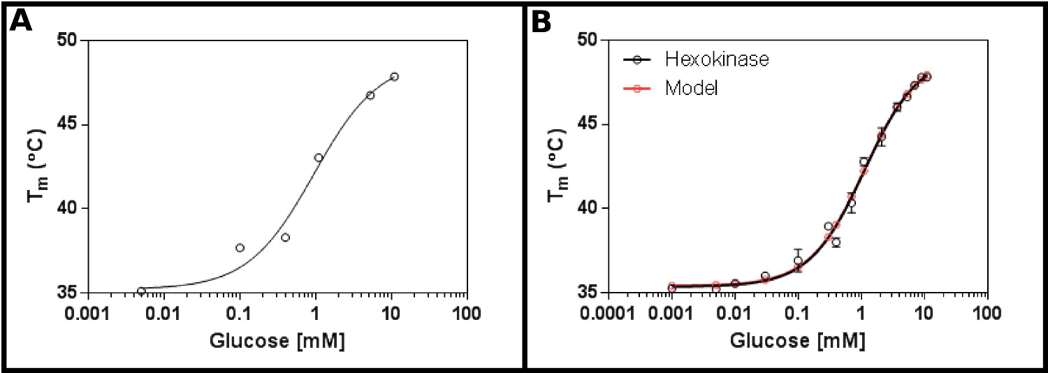
Figure 2. Interaction of hexokinase with glucose measured by differential scanning fluorimetry. (A) An initial experiment testing a wide range of glucose concentrations suggests that the K_d is likely to be in the range of 0.2 - 1.7 mM. (B) A detailed experiment, testing 16 concentrations of glucose, allows determination of the apparent K_d as 1.12 ± 0.05 mM. The data fits extremely well to the model for a single binding event (with the bottom (T1) and top (T2) temperatures fitting to 35.4 ± 0.2 ºC and 49.3 ± 0.5 ºC respectively). Note that these data were collected in the presence of 10 mM MgCl₂. These images were prepared using GraphPad. Please click here to view a larger version of this figure.

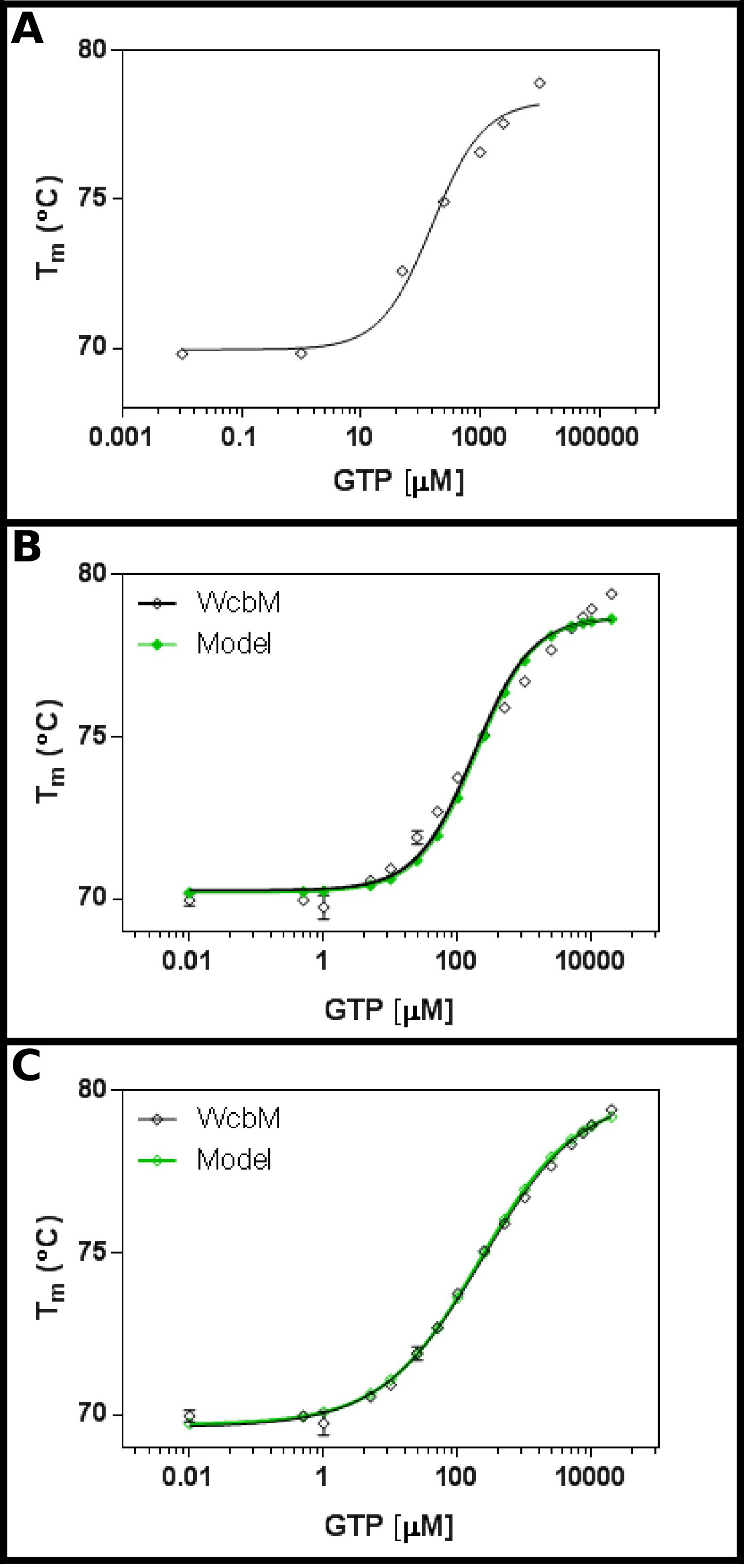
Figure 3. Interaction of WcbM with GTP reveals an anti-cooperative binding. (A) An initial experiment testing a wide range of GTP concentrations suggests that the K_d is likely to be in the range of 200 - 500 µM. (B) A detailed experiment, testing 16 concentrations of GTP, suggests a value for the apparent K_d of 120 ± 20 µM. However, when a logarithmic scale is used for the x-axis, there is a significant discrepancy between the model and data. (C) Analysis of the same data with a cooperative model shows an excellent fit to the data where a simple cooperative model is used. Here, a K_½ of 230 ± 20 µM was determined, with the cooperativity coefficient n = 0.52 ± 0.02 (with the bottom (T1) and top (T2) temperatures fitting to 69.63 ± 0.06 ºC and 79.9 ± 0.1 ºC respectively). As WcbM appears to be dimeric, this implies that the enzyme is perfectly anticooperative in its binding to GTP. These images were prepared using GraphPad. Please click here to view a larger version of this figure.

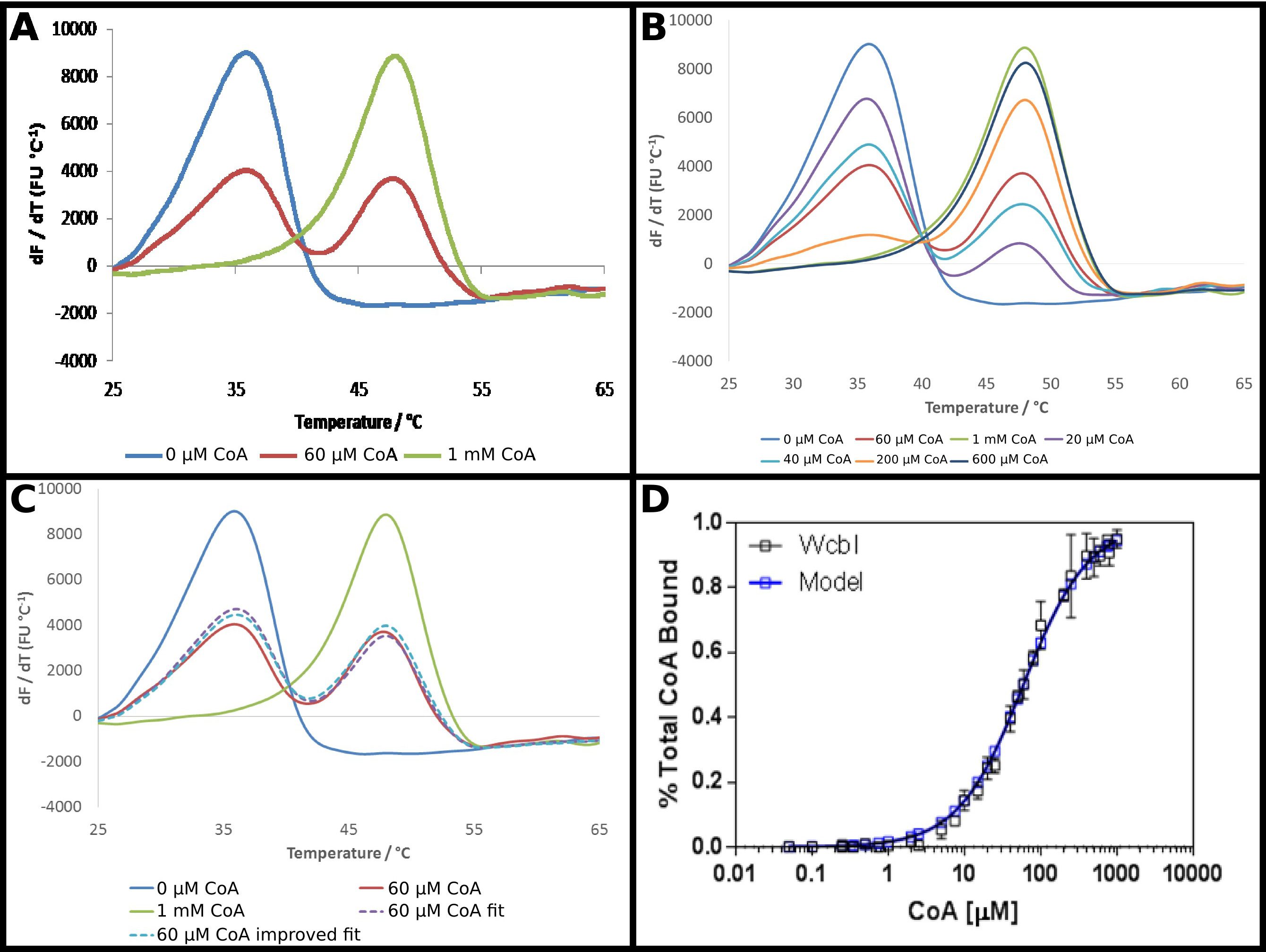
Figure 4. WcbI shows a biphasic melting pattern in the presence of its ligand coenzyme A (CoA). (A) WcbI, in the absence of ligand (blue), shows a simple monophasic melting pattern. At high ligand concentrations (1 mM; green line), a similar pattern is observed. However, at intermediate ligand concentrations (60 µM; red line), two distinct melting peaks, corresponding to ligand-free and ligand-bound states are observed. (B) The transition between the two sets of peaks is dose-dependent across the full range of concentrations. (C) Modelling of the biphasic melting as a sum of a proportion of the ligand free and high ligand results gives a good fit to the data (dashed purple line, compared with red line). This fit is improved by extrapolating the result observed for high ligand concentration (where the model suggests ~95% occupancy) to full occupancy (dashed blue line). (D) The data obtained for the proportion of WcbI bound to CoA shows an excellent fit to a simple binding model, with a K_d of 58 ± 2 µM (these data represent data collected on two separate days, with slightly different ligand concentrations chosen for the second day based on the first set of results). Panels (A - C) were prepared using Excel, and panel (D) using Graphpad. Please click here to view a larger version of this figure.

Table 1. Recipe for initial experiments.

Reagent	Volume in mix (µl)
Protein	To final concentration of 0.11 mg/ml
5000X SYPRO Orange	0.3
0.5 M HEPES pH 7.0	3.7
5 M NaCl	5.6
Water	To 180 µl

This describes the “master mix” of protein, detection reagent and buffer for an initial scouting experiment to provide an estimate of K_d, as described in protocol section 1. This buffer mixture is appropriate for generic proteins. Where previous results suggest other buffers should be used, these should be substituted. If the protein stock is at a low concentration (i.e., less than 0.3 mg/ml), it may be necessary to reduce the amount of additional buffer added to compensate for buffer already present in the protein sample.

Table 2. Recipe for determination of K_d.

Reagent	Volume in mix (µl)
Protein	To final concentration of 0.11 mg/ml
5,000X SYPRO Orange	1.78
0.5 M HEPES pH 7.0	22.2
5 M NaCl	33.3
Water	To 180 µl

This describes the “master mix” of protein, detection reagent, and buffer for a full determination of K_d for a protein sample, as described in protocol section 2. This buffer mixture is appropriate for generic proteins. Where previous results suggest other buffers should be used, these should be substituted. If the protein stock is at a low concentration (i.e., less than 0.3 mg/ml), it may be necessary to reduce the amount of additional buffer added to compensate for buffer already present in the protein sample.

Table 3. Equations and parameters for data analysis.

Step in experimental protocol	Equation required	Parameters required	Description of variables and parameters
3.3
Single site ligand binding	Y=Bottom + ((Top-Bottom)*(1-((P-Kd-X+sqrt(((P+X+Kd)^2)-(4*P*X)))/(2*P))))		P: protein concentration. Kd:  dissociation constant. P and Kd are given in the same units that were used for the ligand concentrations. Top, Bottom: melting temperatures at infinite ligand concentration and no ligand concentration respectively.
3.4		Bottom = *YMIN	YMIN: Minimum value of Y (lowest experimental protein Tm, in this case)
		Top = *YMAX	YMAX: Maximum value of Y (highest experimental protein Tm)
		Kd = *X at YMID	YMID: value of Y that corresponds to the mean of YMIN and YMAX. X is the corresponding X value (here, the relevant ligand concentration)
		P = (Initial value, to be fit)
4.1
Simple cooperative model	Y=Bottom+((Top-Bottom)*(((X/Kd)^n)/(1+((X/Kd)^n))))		n: Hill coefficient. This describes the cooperativity, or other biochemical properties, of the protein, and is not necessarily an estimate of the number of ligand binding sites in the protein. A Hill coefficient of one represents no cooperativity; values lower than one indicate negative cooperativity, and values greater than one positive cooperativity.
		Bottom = *YMIN
		Top = *YMAX
		Kd = *X at YMID
		P = (Initial value, to be fit)
		n = (Initial value, to be fit)
Sequential binding of two ligands	Y=Bottom+((Top-Bottom)*((X^2)/(Kd*K2))/(1+(X/Kd)+((X^2)/(Kd*K2))))		K2: dissociation constant for second binding event.
		Bottom = *YMIN
		Top = *YMAX
		Kd = *X at YMID
		K2  = *X at YMID
		P = (Initial value, to be fit)
Independent binding of two ligands	Y=Bottom+((Top-Bottom)*((X^2)/(Kd*K2))/(1+(2*X/Kd)+((X^2)/(Kd*K2))))
		Bottom = *YMIN
		Top = *YMAX
		Kd = *X at YMID
		K2  = *X at YMID
		P = (Initial value, to be fit)
5.5
Analysis of binary shifts in melting temperature	Y=1-((P-Kd-X+sqrt(((P+X+Kd)^2)-(4*P*X)))/(2*P))
		Bottom = *YMIN
		Top = *YMAX
		Kd = *X at YMID
		P = (Initial value, to be fit)
5.8
Extrapolation to infinite ligand concentration	(C2-((1-$R$2)*B2))/$R$2		B2:  cell containing the result with no ligand. C2:  cell containing the result with maximum ligand. $R$2: cell containing the proportion bound at maximum ligand concentration.

Steps 3, 4 and 5 require the addition of detailed equations into the analysis software, and precise definition of starting parameters for data analysis. The equations for each relevant step are shown, with the correct selections of the parameters. An explanation of the meaning of variables and parameters is provided for reference.

Table 4. Concentrations for screening of interaction of hexokinase with glucose.

Sample point	Ligand (glucose) concentration (mM)
1	0
2	0.001
3	0.005
4	0.01
5	0.03
6	0.1
7	0.3
8	0.4
9	0.7
10	1.1
11	2.1
12	3.7
13	5.3
14	7
15	9
16	11

Hexokinase from the budding yeast Saccharomyces cerevisiae was added to the master mix as described in the protocol, supplemented with 10 mM MgCl₂ as magnesium is a known cofactor. The initial estimate of the K_d was between 0.5 and 2 mM. Experiments were set up to provide the indicated final concentrations of glucose.

Table 5. Concentrations for screening of interaction of WcbM with GDP.

Sample point	Ligand (GTP) concentration (μM)
1	0
2	0.5
3	1
4	5
5	10
6	25
7	50
8	100
9	250
10	500
11	1,000
12	2,500
13	5,000
14	7,500
15	10,000
16	20,000

WcbM from Burkholderia pseudomallei was added to the master mix as described in the protocol. The initial estimate of the K_d was around 100 µM. Experiments were set up to provide the indicated final concentrations of GTP, aiming to cover at least two orders of magnitude above and below K_d.

Discussion

Differential scanning fluorimetry has demonstrated its power as a robust and versatile method for characterizing proteins, and identifying potential protein ligands. The well documented successes in expediting protein stabilization, drug discovery (especially in less well financed laboratories) and crystallization ^10,23-25 have made it an attractive method for initial screening of compounds. Compounds added to proteins show a clear dose dependent increase in the apparent melting temperature ^7,9. However, there have been few attempts to use the results from these experiments to determine apparent binding constants to aid in ranking compounds for their affinity. Here, we present a method for systematically determining an apparent dissociation constant for proteins in the presence of a ligand.

The results presented here demonstrate that DSF can rapidly and robustly provide estimates of the dissociation constant for a protein-ligand combination. The observed data can be manipulated with commercially available tools to provide a rapid determination of K_d, without the need to make assumptions regarding the likely value of parameters. The method has a significant advantage over some comparable methods of being parsimonious in both protein and time required. The experiment described here will consume 0.13 mg of protein per experiment (approximately 0.4 mg for experiments repeated in triplicate). This compares favorably with isothermal titration calorimetry (ITC), where a single experiment with an average 40 kDa protein will consume a similar amount. The full set of experiments required for this protocol would consume around 4 hr, including preparation, for a single set of experiments. Again, this is likely to be considerably quicker than methods such as ITC or surface plasmon resonance, which whilst powerful often require considerable optimization to achieve best data.

Our results demonstrate that there remains a requirement to carefully examine the raw data, the fit of these data to determine the melting temperature, and the fit of the melting temperature data to determine the dissociation constant. A first challenge is the shape of the raw data produced in the protein melting. In some cases, the shape may not approximate to that observed in Figure 1A. Common issues include low temperature shifts on ligand binding, high background fluorescence, and unusual multiple transitions in temperature. Low temperature shifts are seen on binding a number of ligands. For this method, the most critical parameter is the error in the T_m measurement, compared to the temperature shift. The data can usually be fitted reasonably well when the standard deviation of triplicate measurements do not exceed 10% of the melting temperature shift between unbound and fully bound protein. Our experience is that where such temperature shifts are only 2 °C, this can be sufficient for fitting the data, if the individual data points are highly accurate. A second issue is unusually shaped curves. These often differ between free protein and ligand bound forms, as the ligand binding affects unfolding modes of the protein. In these cases, the user must consider whether the data can be used with appropriate consideration of the models to be used for determining the melting temperature and the dissociation constant. Another common issue is that addition of a cofactor to the protein (e.g., MgCl₂ in our example with hexokinase) is required to obtain the most reliable data. Our experience has been that careful consideration of all likely factors in the experiment at the stage of taking initial readings is essential to obtaining the best results. Furthermore, alternative theoretical treatments can reveal features of these data ^15,17. Finally, it is not uncommon for some proteins that contain natively exposed hydrophobic regions to show high background fluorescence. There are a number of solutions to these problems, which have been extensively reviewed elsewhere^6,9.

In particular, the user must consider whether to use the Boltzmann or derivative models (e.g., Figure 4), and in the case of use of derivatives, whether multiple melts must be modelled. The two methods of modeling the thermal unfolding differ in that the Boltzmann method fits the experimental data to the Boltzmann equation, assuming a regular sigmoidal shape to the unfolding curve. In contrast, the derivative method takes the first derivative of the experimental data at each point (lower panel in Figure 1A), and considers the melting temperature to be the point of highest first derivative. The derivative method generally returns a higher melting temperature by around 2 - 3 °C. Most proteins will return a more consistent result (i.e., the standard error of the melting temperature for triplicate experiments is lower) for one of the two methods. This is usually intimately related to the precise shape of the protein unfolding curve, and it is necessary to empirically determine the best method in each case. Where the derivative model is used, it is also important to consider multiple melting events. Some data clearly show evidence for multiple transitions, and in these cases the results are likely to be easier to interpret if these multiple melting events are modelled. In the context of this protocol, it is often the case that the addition of ligand can cause a protein to shift from having multiple melting transitions to a single transition (e.g., by stabilizing the most thermally fragile subdomain), or vice versa. We would therefore advocate that the raw data are examined together before considering which approach will be best to use.

Following the modelling of the individual melting temperatures, further issues can arise in fitting these to the models presented in the protocol section. It is imperative to carefully examine the fit to the dissociation constant equation using a logarithmic scale, as this analysis often highlights discrepancies between the observed data and the model (e.g., Figure 3). Whilst the results obtained are generally robust, care in interpretation offers the opportunity to extract better results, and the most meaning, from the data.

A particular issue raised by these data is the interpretation that should be placed on proteins that show cooperativity, or multiple binding events, in DSF. We have, to date, only observed this phenomenon in proteins that are expected to have multiple specific binding events (e.g., WcbM, a protein whose best homologue is a multimer ²⁶, and which acts as a multimer on size exclusion chromatography [data not shown]). It is not at all clear that the negative cooperativity observed in DSF denaturation indicates that the enzyme will ultimately show negative cooperativity: rather, this may be an indication of complex binding that must be explored more thoroughly using a wider range of methods. This does suggest to us, however, that more extensive studies of such proteins are likely to identify interesting effects.

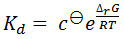
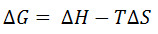
The values given for the dissociation constant using this method are generally of the same order as those provided by other methods, such as isothermal titration calorimetry and surface plasmon resonance. However, the absolute values observed are frequently higher than observed using these methods. This is at least partly a consequence of the fact that the dissociation constant is observed at the melting temperature of the protein with ligand. This K_d is generally higher than that at physiological temperatures. The dissociation constant is related to the temperature of the reaction by the equations:

[1]

[2]

(where c^θ is the standard reference concentration, Δ_rG is the Gibbs free energy change of the reaction, R is the molar gas constant, ΔH is the enthalpy change in the reaction, and ΔS is the entropy change in the reaction.)

Reactions with dissociation constants in the measurable range of this method will generally have a negative Δ_rG, and so the effect of an increase in temperature on equation [1] will be to increase the dissociation constant. Both the ΔH and ΔS terms that constitute the Gibbs free energy (equation [2]) are temperature dependent²⁷, and the effect on the dissociation constant will depend on the magnitude and sign of these temperature dependencies, and will necessarily be interaction dependent. Consequently, it is not unexpected that the dissociation constants determined by this method are sometimes greater than those determined by methods that operate at RT. Temperature dependence is, of course, also a caveat of many other methods, which tend to provide the dissociation constant at temperatures lower than the physiological temperature.

Another caveat of the DSF method is that it is a labeled method, unlike ITC. The fluorescent label used (SYPRO Orange) is hydrophobic, and so in some cases can compete with the binding of hydrophobic ligands to proteins. Consequently, it is likely that in some cases, the dissociation constant obtained will be artificially raised due to competition with the label. However, for the comparison of diverse ligands, (the primary use of DSF), the differences are unlikely to be sufficiently significant to affect the ranking of compounds by affinity.

A potential drawback of this method is the limit of detection that can be achieved. In principle, it should not be possible to accurately measure a value for K_d that is lower than 50% of the protein concentration, and even values in this range are likely to be of dubious accuracy. Whilst the limit of detection at this end of the range may be extended a little by reducing the concentrations of protein and dye, the sensitivity of the instrument will prevent further reduction in protein concentration. Similarly, the upper end of the sensitivity will be determined by the solubility of the ligand. To obtain a mathematically robust estimate for K_d, it is most important to obtain data with 90% of the protein present in the ligand-bound form, which requires ligand concentrations to be approximately ten times K_d (assuming no cooperativity). The limit of detection will therefore necessarily be one tenth of the solubility of the ligand in the relevant buffer. This means that the limits of detection of the method will typically range between 1 µM and between 1 and 100 mM, depending on the protein and ligand.

In conclusion, differential scanning fluorimetry is a versatile technique applicable to a wide range of proteins. Using the methods presented here, it is possible to rapidly and inexpensively determine the affinity of a protein for different ligands. This has great potential for application in protein purification and stabilization, elucidating the function or specificity of enzymes from metagenomes, and in drug discovery, especially in small laboratories.

Materials

List of materials used in this article

Name	Company	Catalog Number	Comments
StepOne real time PCR instrument	Life Technologies	4376357	DSF can be performed with many other instruments. The StepOne instrument has very convenient software for data analysis.
Protein thermal shift software v1.0	Life Technologies	4466037
MicroAmp Fast optical 48-well plates	Life Technologies	4375816
Optical sealing tape	Life Technologies	4375323	Bio-rad part no. 223-9444 is an alternative supplier
U-bottomed 96-well plates	Fisher	11521943
SYPRO Orange	Life Technologies	S6650	For a smaller volume supplier, use Sigma part no. S5692
SPSS statistics version 20	IBM		Other statistics packages will provide similar functionality
GraphPad Prism 6.02	GraphPad		Other statistics packages will provide similar functionality
Hand applicator (PA1)	3M	75-3454-4264-6
Hexokinase from Saccharomyces cerevisiae	Sigma-Aldrich	H5000
Glucose	Fisher scientific	10141520

References

- Freyer, M. W., Lewis, E. A. Isothermal titration calorimetry: experimental design, data analysis, and probing macromolecule/ligand binding and kinetic interactions. Methods Cell Biol. 84, 79-113 (2008).
- Ladbury, J. E. Calorimetry as a tool for understanding biomolecular interactions and an aid to drug design. Biochem Soc Trans. 38, 888-893 (2010).
- Abdiche, Y., Malashock, D., Pinkerton, A., Pons, J. Determining kinetics and affinities of protein interactions using a parallel real-time label-free biosensor, the Octet. Anal Biochem. 377, 209-217 (2008).
- Pantoliano, M. W., et al. High-density miniaturized thermal shift assays as a general strategy for drug discovery. J Biomol Screen. 6, 429-440 (2001).
- Senisterra, G., Chau, I., Vedadi, M. Thermal denaturation assays in chemical biology. Assay Drug Dev Technol. 10, 128-136 (2012).
- Ericsson, U. B., Hallberg, B. M., Detitta, G. T., Dekker, N., Nordlund, P. Thermofluor-based high-throughput stability optimization of proteins for structural studies. Anal Biochem. 357, 289-298 (2006).
- Lo, M. C., et al. Evaluation of fluorescence-based thermal shift assays for hit identification in drug discovery. Anal Biochem. 332, 153-159 (2004).
- Nettleship, J. E., Brown, J., Groves, M. R., Geerlof, A. Methods for protein characterization by mass spectrometry, thermal shift (ThermoFluor) assay, and multiangle or static light scattering. Methods Mol Biol. 426, 299-318 (2008).
- Niesen, F. H., Berglund, H., Vedadi, M. The use of differential scanning fluorimetry to detect ligand interactions that promote protein stability. Nat Protoc. 2, 2212-2221 (2007).
- Geders, T. W., Gustafson, K., Finzel, B. C. Use of differential scanning fluorimetry to optimize the purification and crystallization of PLP-dependent enzymes. Acta Crystallogr Sect F Struct Biol Cryst Commun. 68, 596-600 (2012).
- Vedadi, M., et al. Chemical screening methods to identify ligands that promote protein stability, protein crystallization, and structure determination. Proc Natl Acad Sci USA. 103, 15835-15840 (2006).
- Davis, B. J., Erlanson, D. A. Learning from our mistakes: the 'unknown knowns' in fragment screening. Bioorg Med Chem Lett. 23, 2844-2852 (2013).
- Larsson, A., Jansson, A., Aberg, A., Nordlund, P. Efficiency of hit generation and structural characterization in fragment-based ligand discovery. Curr Opin Chem Biol. 15, 482-488 (2011).
- Scott, D. E., et al. Using a fragment-based approach to target protein-protein interactions. Chembiochem. 14, 332-342 (2013).
- Cimmperman, P., et al. A quantitative model of thermal stabilization and destabilization of proteins by ligands. Biophys. J. 95, 3222-3231 (2008).
- Matulis, D., Kranz, J. K., Salemme, F. R., Todd, M. J. Thermodynamic stability of carbonic anhydrase: measurements of binding affinity and stoichiometry using ThermoFluor. Biochemistry. 44, 5258-5266 (2005).
- Zubriene, A., et al. Measurement of nanomolar dissociation constants by titration calorimetry and thermal shift assay - radicicol binding to Hsp90 and ethoxzolamide binding to CAII. Int J Mol Sci. 10, 2662-2680 (2009).
- Weiss, J. N. The Hill equation revisited: uses and misuses. FASEB J. 11, 835-841 (1997).
- Cuccui, J., et al. Characterization of the Burkholderia pseudomallei K96243 capsular polysaccharide I coding region. Infect Immun. 80, 1209-1221 (2012).
- DeShazer, D., Waag, D. M., Fritz, D. L., Woods, D. E. Identification of a Burkholderia mallei polysaccharide gene cluster by subtractive hybridization and demonstration that the encoded capsule is an essential virulence determinant. Microb Pathog. 30, 253-269 (2001).
- Berman, H., Henrick, K., Nakamura, H. Announcing the worldwide Protein Data Bank. Nat Struct Biol. 10, 980(2003).
- Vivoli, M., Ayres, E., Beaumont, E., Isupov, M., Harmer, N. Structural insights into WcbI, a novel polysaccharide biosynthesis enzyme. IUCr Journal. 1 (1), 28-38 (2014).
- Sorrell, F. J., Greenwood, G. K., Birchall, K., Chen, B. Development of a differential scanning fluorimetry based high throughput screening assay for the discovery of affinity binders against an anthrax protein. J Pharm Biomed Anal. 52, 802-808 (2010).
- Uniewicz, K. A., et al. Differential scanning fluorimetry measurement of protein stability changes upon binding to glycosaminoglycans: a screening test for binding specificity. Anal Chem. 82, 3796-3802 (2010).
- Wan, K. F., et al. Differential scanning fluorimetry as secondary screening platform for small molecule inhibitors of Bcl-XL. Cell Cycle. 8, 3943-3952 (2009).
- Koropatkin, N. M., Holden, H. M. Molecular structure of alpha-D-glucose-1-phosphate cytidylyltransferase from Salmonella typhi. J Biol Chem. 279, 44023-44029 (2004).
- Paleskava, A., Konevega, A. L., Rodnina, M. V. Thermodynamics of the GTP-GDP-operated conformational switch of selenocysteine-specific translation factor SelB. J Biol Chem. 287, 27906-27912 (2012).
Reprints and Permissions
Request permission to reuse the text or figures of this JoVE article
Request Permission