Using Light Sheet Fluorescence Microscopy to Image Zebrafish Eye Development

Summary

Light sheet fluorescence microscopy is an excellent tool for imaging embryonic development. It allows recording of long time-lapse movies of live embryos in near physiological conditions. We demonstrate its application for imaging zebrafish eye development across wide spatio-temporal scales and present a pipeline for fusion and deconvolution of multiview datasets.

Abstract

Light sheet fluorescence microscopy (LSFM) is gaining more and more popularity as a method to image embryonic development. The main advantages of LSFM compared to confocal systems are its low phototoxicity, gentle mounting strategies, fast acquisition with high signal to noise ratio and the possibility of imaging samples from various angles (views) for long periods of time. Imaging from multiple views unleashes the full potential of LSFM, but at the same time it can create terabyte-sized datasets. Processing such datasets is the biggest challenge of using LSFM. In this protocol we outline some solutions to this problem. Until recently, LSFM was mostly performed in laboratories that had the expertise to build and operate their own light sheet microscopes. However, in the last three years several commercial implementations of LSFM became available, which are multipurpose and easy to use for any developmental biologist. This article is primarily directed to those researchers, who are not LSFM technology developers, but want to employ LSFM as a tool to answer specific developmental biology questions.

Here, we use imaging of zebrafish eye development as an example to introduce the reader to LSFM technology and we demonstrate applications of LSFM across multiple spatial and temporal scales. This article describes a complete experimental protocol starting with the mounting of zebrafish embryos for LSFM. We then outline the options for imaging using the commercially available light sheet microscope. Importantly, we also explain a pipeline for subsequent registration and fusion of multiview datasets using an open source solution implemented as a Fiji plugin. While this protocol focuses on imaging the developing zebrafish eye and processing data from a particular imaging setup, most of the insights and troubleshooting suggestions presented here are of general use and the protocol can be adapted to a variety of light sheet microscopy experiments.

Introduction

Morphogenesis is the process that shapes the embryo and together with growth and differentiation drives the ontogeny from a fertilized egg into a mature multicellular organism. The morphogenetic processes during animal development can be analyzed best by imaging of intact living specimens^1-3. This is because such whole embryo imaging preserves all the components that drive and regulate development including gradients of signaling molecules, extracellular matrix, vasculature, innervation as well as mechanical properties of the surrounding tissue. To bridge the scales, at which morphogenesis occurs, the fast subcellular events have to be captured on a minute time scale in the context of development of the whole tissue over hours or days. To fulfill all these requirements, a modern implementation⁴ of the orthogonal plane illumination microscope⁵ was developed. Originally, it was named the Selective Plane Illumination Microscopy (SPIM)⁴; now an all-embracing term Light Sheet Fluorescence Microscopy (LSFM) is typically used. LSFM enables imaging at high time resolution, while inducing less phototoxicity than laser scanning or spinning disc confocal microscopes^6,7. Nowadays, there are already many implementations of the basic light sheet illumination principle and it has been used to image a large variety of specimens and processes previously inaccessible to researchers^8-11.

We would first like to highlight several key advantages of LSFM over conventional confocal microscopy approaches:

To acquire meaningful results from live imaging microscopic experiments, it is important that the observation only minimally affects the specimen. However, many organisms including zebrafish are very susceptible to laser light exposure, making it challenging to image them in a confocal microscope with high time resolution without phototoxicity effects like stalled or delayed development^6,7. LSFM is currently the fluorescence imaging technique with the least disruptive effects on the sample⁷. Since the thin laser light sheet illuminates only the part of the specimen that is imaged at a particular time point, the light sheet microscope is using photons very efficiently. Consequently, the low light exposure allows for longer time-lapse observations of healthier specimens, e.g.^12-17. Furthermore, thanks to the minimal invasiveness of LSFM, the number of acquired images is no longer dictated by how much light the sample can tolerate, but rather by how much data can be processed and stored.

Along the same lines of keeping the specimen in near physiological conditions, LSFM comes with alternative sample mounting strategies well suited for live embryos. In LSFM techniques, the embryos are typically embedded within a thin column of low percentage agarose. The mounting into agarose cylinders allows for the complete freedom of rotation, so the sample can be observed from the perfect angle (in LSFM referred to as view) and from several views simultaneously. The multiview imaging and subsequent multiview fusion is beneficial particularly for big, scattering specimens and allows capturing them with high, isotropic resolution. A summary of other possible LSFM mounting strategies can be found in the official microscope operating manual, in the chapter on sample preparation written by the lab of E. Reynaud. It is a recommended read, especially if the goal is to image different samples than described here.

The image acquisition in LSFM is wide field, camera-based, as opposed to laser scanning confocal microscope. This results in a higher signal-to noise ratio (SNR) for acquired images and can be extremely fast (tens to hundreds of frames per second). The high sensitivity of LSFM further enables imaging of weakly fluorescent samples, like transcription factors expressed at endogenous levels¹⁸ or, in the near future, endogenous proteins tagged using CRISPR/Cas9. The high SNR is also important for successful downstream image analysis. The high speed is required not only to capture rapid intracellular processes, but also to image the whole embryo from multiple views fast enough. A seamless fusion of the multiple views can only be achieved, if the observed phenomenon does not change during acquisition of these several z stacks coming from separate views.

The advantages of LSFM do not typically come at the expense of image quality. The lateral resolution of LSFM is slightly worse than the resolution of a confocal microscope. This is because the detection objectives used in LSFM have lower numerical aperture (usually 1.0 or less) compared to 1.2-1.3 of water or silicon immersion objectives on standard confocal setups. Additionally, due to the wide field detection in LSFM (absence of a pinhole), there is more out-of-focus light compared to a confocal microscope. The amount of out-of-focus light is determined by the light sheet thickness. Nevertheless, these disadvantages are compensated by the higher SNR in LSFM. In practice, this results in similar quality images compared to for example spinning disc confocal acquisition¹⁵. Consequently, this enables reliable extraction of features like cell membranes or nuclei, e.g., for cell lineage tracing^15,19.

The axial resolution of LSFM is determined, in addition to the detection objective, by the light sheet thickness. The axial resolution of LSFM can in some cases surpass the resolution of confocal microscopes. First, the improvement in resolution comes when the light sheet is thinner than the axial resolution of the detection objective, which typically occurs for large specimens imaged with a low magnification objective. The second way, how the LSFM can achieve better axial resolution, is the multiview fusion, in which the high xy resolution information from different views is combined into one image stack. The resulting merged stack has an isotropic resolution approaching the values of resolution in the lateral direction^20,21. The strategy for registering the multiple views onto each other described in this article is based on using fluorescent polystyrene beads as fiduciary markers embedded in the agarose around the sample^20,21.

As a result of the LSFM commercialization, this technique is now available to a broad community of scientists²². Therefore, the motivation for writing this protocol is to make this technology accessible to developmental biologists lacking practical experience in LSFM and to get these scientists started using this technology with their samples. Our protocol uses the commercial light sheet microscope, which constitutes a conceptually simple microscope that is easy to operate. We would additionally like to mention other recent protocols for imaging zebrafish with home-built LSFM setups, which might be suitable to answer particular questions^23-25. Another entry option to LSFM are the open platforms^26,27, which use the open access principles to bring light sheet microscopy to a broader community. The documentation of both the hardware and the software aspects can be found at http://openspim.org and https://sites.google.com/site/openspinmicroscopy/.

In this protocol, we use the teleost zebrafish as a model system to study developmental processes with LSFM. Morphogenesis of the zebrafish eye is an example that underlines many of the benefits of LSFM. LSFM has already been used in the past to investigate eye development in medaka²⁸ and in zebrafish^29,30. At the early stage of eye development it is complicated to orient the embryo correctly for conventional microscopy, as the bulky yolk does not allow the embryo to lie on the side with its eye facing the objective. However, with LSFM mounting into an agarose column, the sample can be reproducibly positioned. Additionally, during the transition from optic vesicle to the optic cup stage, the eye undergoes major morphogenetic rearrangements accompanied by growth, which requires capturing a large z stack and a big field of view. Also for these challenges LSFM is superior to conventional confocal imaging. The process of optic cup formation is three-dimensional, therefore it is hard to comprehend and visualize solely by imaging from one view. This makes multiview imaging with isotropic resolution beneficial. After optic cup formation, the retina becomes increasingly sensitive to laser exposure. Thus, the low phototoxicity associated with LSFM is a major advantage for long-term imaging.

Here we present an optimized protocol for imaging of one to three days old zebrafish embryos and larvae with focus on the eye development. Our method allows recording of time-lapse movies covering up to 12-14 hr with high spatial and temporal resolution. Importantly, we also show a pipeline for data processing, which is an essential step in LSFM, as this technique invariably generates big datasets, often in the terabyte range.

Protocol

NOTE: All animal work was performed in accordance with European Union (EU) directive 2011/63/EU and the German Animal Welfare Act. The protocol is meant to be followed without interruption, from mounting to imaging the sample. Depending on the practical experience, it will take 2-3 hr to start a time-lapse experiment. Data processing is not included in this time calculation. All the material required for the experiment can be found in the checklist of material needed before starting that is provided as a supplementary document. Wear powder free gloves during the steps 1, 2, 3 and 4. For steps 2, 3, 4 and 5 of the protocol also refer to the official microscope operating manual.

1. Preparatory Work Before the Imaging Experiment

1. Fluorescent Bead Stock Solution
   1. For this protocol, use the 500 or 1,000 nm diameter polystyrene beads (labeled with red emitting fluorescent dye). The working dilution of the beads is 1:4,000. First, vortex the bead stock solution for 1 min. Dilute 10 µl of beads in 990 µl of ddH₂O. Store the solution in the dark at 4 °C and use this 1:100 dilution as the stock solution for further dilution in 1:40.
2. Preparing Solution for the Sample chamber
   1. In a 100 ml beaker mix 38.2 ml of E3 medium without methylene blue, 0.8 ml of 10 mM N-phenylthiourea and 1 ml of 0.4% MS-222. It is beneficial to use filtered E3 medium to avoid small particles of dust or undissolved crystals floating in the sample chamber later.
3. Fluorescent Fish Embryo Selection
   1. In the days prior to the experiment, prepare embryos expressing fluorescent proteins. Right before the experiment, sort the embryos under the fluorescent stereoscope for desirable strength of the fluorescent signal. Take 5-10 healthy embryos and dechorionate them using tweezers.
      NOTE: This protocol is optimized for 16-72 hr old embryos.

2. Setting Up the Sample Chamber

1. Assembling the Three Chamber Windows
   1. There are 4 windows in the sample chamber, one for the objective and three to be sealed with the coverslips (18 mm diameter, selected thickness 0.17 mm). Store these coverslips in 70% ethanol. Wipe them clean before use with ether:ethanol (1:4).
   2. Insert the coverslip into the window using fine forceps and make sure it fits into the smallest groove. Cover it with the 17 mm diameter rubber O-ring and screw in the illumination adapter ring using the chamber window tool. Repeat the process for the other two windows.
2. Attaching the Remaining Chamber Parts
   1. Screw the adapter for an appropriate objective into the fourth remaining side of the chamber. Insert the 15 mm diameter O-ring into the center of the adapter.
   2. Screw in the white Luer-Lock adapter into the lower right opening in the chamber and the grey drain connector in the upper left opening. Block all the three remaining openings with the black blind plugs.
   3. Attach the Peltier block and the metal dovetail slide bottom of the chamber using an Allen wrench. Attach the hose with the 50 ml syringe to the Luer-Lock adapter. Insert the temperature probe into the chamber.
3. Inserting the Objectives and the Chamber into the Microscope
   1. Check under the stereoscope that all the objectives are clean. Use the 10X/0.2 illumination objectives and the Plan-Apochromat 20X/1.0 W detection objective and make sure that its refractive index correction collar is set to 1.33 for water. Screw the detection objective into the microscope, while keeping the illuminating objectives covered.
   2. Remove the protective plastic caps covering the illuminating objectives. Carefully slide the chamber into the microscope and tighten it with the securing screw.
   3. Connect the temperature probe and the Peltier block with the microscope.
      NOTE: The two tubes that circulate the cooling liquid for the Peltier block are compatible with both connectors. They form a functioning circuit irrespective of the orientation of connection.
   4. Fill the chamber through the syringe with solution prepared in step 1.2 up to the upper edge of the chamber windows. Check that the chamber is not leaking.
   5. Start the microscope, incubation and the controlling and storage computers. Start the microscope-operating software and set the incubation temperature to 28.5 °C.
      NOTE: It will take 1 hr to completely equilibrate. Prepare the sample in the meantime.

3. Sample Preparation

1. Preparing the Agarose Mix
   1. 15 min before making of the agarose mix, melt one 1 ml aliquot of 1% low melting point agarose (dissolved in E3 medium) in a heating block set to 70 °C. Once the agarose is completely molten, transfer 600 µl into a fresh 1.5 ml tube, add 250 µl of E3 medium, 50 µl of 0.4% MS-222 and 25 µl of vortexed bead stock solution.
      NOTE: This makes 925 µl of the mix, while additional 75 µl is calculated for the liquid added later together with the embryos.
   2. Keep the tube in a second heating block at 38-40 °C or ensure that the agarose is very close to its gelling point before putting sample embryos into it.
2. Mounting the Embryos
   1. Take five glass capillaries of 20 µl volume (with a black mark, ~1 mm inner diameter) and insert the matching Teflon tip plungers into them. Push the plunger through the capillary so that the Teflon tip is at the bottom of the capillary.
   2. Transfer five embryos (a number that can be mounted at once) with a glass or plastic pipette into the tube of vortexed 37 °C warm agarose mix.
      NOTE: Try to carry over a minimum volume of liquid together with the embryos.
   3. Insert the capillary into the mix and suck one embryo inside by pulling the plunger up. Ensure that the head of the embryo enters the capillary before the tail. Avoid any air bubbles between the plunger and the sample. There should be ±2 cm of agarose above the embryo and ±1 cm below it. Repeat for the remaining embryos.
   4. Wait until the agarose solidifies completely, which happens within a few minutes and then store the samples in E3 medium, by sticking them to the wall of a beaker with plasticine or tape. The bottom opening of the capillary should be hanging free in the solution allowing gas exchange to the sample.
      NOTE: A similar protocol to the sections 3.1 and 3.2 can be also found on the OpenSPIM wiki page http://openspim.org/Zebrafish_embryo_sample_preparation.

4. Sample Positioning

1. Sample Holder Assembly
   1. Insert 2 plastic sleeves of the right size (black) against each other into the sample holder stem. Their slit sides have to face outwards. Attach the clamp screw loosely by turning it 2-3 rounds. Insert the capillary through the clamp screw and push it through the holder until the black color band becomes visible on the other side. Avoid touching the plunger.
   2. Tighten the clamp screw. Push the excess 1 cm of agarose below the embryo out of the capillary and cut it. Insert the stem into the sample holder disc.
   3. Confirm in the software that the microscope stage is in the load position. Use guiding rails to glide the whole holder with the sample vertically downwards into the microscope. Turn it, so that the magnetic holder disc locks into position.
2. Locating the Capillary
   1. From now on, control the sample positioning by the software. In the Locate tab choose the Locate capillary option and position the capillary in x, y and z into focus just above the detection objective lens. Use the graphical representation in the specimen navigator for guidance.
   2. Push the embryo gently out of the capillary until it is in front of the pupil of the detection objective.
      NOTE: The 'Locate capillary' is the only step in the remaining protocol, during which the upper lid of the microscope should be opened and the sample pushed out.
3. Locating the Sample
   1. Switch to 'Locate sample' option and at 0.5 zoom bring the zebrafish eye into the center of the field of view. Rotate the embryo, so that the light sheet will not pass through any highly refractive or absorbing parts of the specimen before it reaches the eye. Likewise, the emitted fluorescence needs a clear path out of the specimen. Click on 'Set Home Position'.
   2. Open the front door of the microscope and put the plastic cover with a 3 mm opening on top of the chamber to avoid evaporation.
      NOTE: If the liquid level drops below the imaging level, the experiment will be compromised.
   3. Check the heartbeat of the embryo as a proxy for overall health. If it is too slow, use another sample (compare to non-mounted controls; specific values depend on developmental stage). Switch to final zoom setting and readjust the position of the embryo.

5. Setting up a Multidimensional Acquisition

1. Acquisition Parameters
   1. Switch to the 'Acquisition' tab. Define the light path including laser lines, detection objective, laser blocking filter, beam splitter and the cameras.
   2. Activate the pivot scan checkbox. Define the other acquisition settings like the bit depth, image format, light sheet thickness and choose single sided illumination.
   3. Press 'Continuous' and depending on the intensity of the obtained image change the laser power and camera exposure time.
      NOTE: For adjusting all the imaging settings use less laser power (0.5% of 100 mW laser, 30 msec exposure time), than for the actual experiment to avoid unnecessary photo damage to the specimen.
2. Light Sheet Adjustment
   1. Switch to the 'Dual Sided Illumination' and activate the 'Online Dual Side Fusio'n checkbox. Start the 'Lightsheet Auto-adjust wizard'. Follow the instructions step by step.
      NOTE: The wizard moves the light sheet into the focal plane of the detection objective, and ensures that it is not tilted and its waist is in the center of the field of view. After finishing the automatic adjustment, the positions of the left and right light sheets are automatically updated in the software. An improvement in image quality should now be apparent. Activate the 'Z-stack' checkbox.
   2. Check the light sheet adjustment by inspecting the symmetry of the point spread function (PSF) given by the fluorescent beads in the xz and yz ortho view. If it is not symmetric, manually adjust the light sheet parameter position up and down until achieving a symmetric hourglass shaped PSF (Figure 1A).
3. Multidimensional Acquisition Settings
   1. Define the z-stack with the 'First Slice' and 'Last Slice' options and set the z step to 1 µm.
      NOTE: The light sheet in this microscope is static and the z sectioning is achieved by moving the sample through. Always use the 'Continuous Drive' option for faster acquisition of z-stacks.
   2. Activate the 'Time Series' checkbox. Define the total number of time points and the interval in between them.
   3. Activate the 'Multiview' checkbox. Add the current view into the multiview list, where the x, y, z and angle information is stored. Use the stage controller to rotate the capillary and define the other desired views. Set up a z-stack at each view and add them to the multiview list.
      NOTE: The software sorts the views in a serial fashion, so that the capillary is turned unidirectionally, while the image is acquired.
4. Drift Correction and Starting the Experiment
   1. Once the acquisition set up is complete, wait 15-30 min before starting the actual experiment.
      NOTE: The sample initially drifts a few micrometers in x, y and z, but should stop within 30 min. If the sample keeps drifting for longer, use another sample or remount.
   2. Switch to the 'Maintain' tab and in the 'Streaming' option define how the data should be saved, e.g., one file per time point or separate file for each view and channel. Go back to the 'Acquisition' tab, press 'Start Experiment' and define the file name, location where it should be saved and the file format (use .czi).
   3. Observe the acquisition of the first time point to confirm that everything is running flawlessly. Immediately proceed with registration and fusion of the first time point as described in steps 6 and 7, to confirm that it will be possible to process the whole dataset.

6. Multiview Registration

1. Multiview Reconstruction Application
   1. At the end of the imaging session, transfer the data from the data storage computer at the microscope to a data processing computer. Use the 'MultiView ReconstructionApplication'^20,21,31 implemented in Fiji³² for data processing (Figure 1B).
2. Define Dataset
   1. Update Fiji: Fiji > Help > Update ImageJ and Fiji > Help > Update Fiji. Use the main ImageJ and Fiji update sites.
   2. Transfer the entire dataset into one folder. The results and intermediate files of the processing will be saved into this folder. Start the MultiView Reconstruction Application: Fiji > Plugins > Multiview Reconstruction > Multiview Reconstruction Application.
   3. Select 'define a new dataset'. As type of dataset select the meu option "Zeiss Lightsheet Z.1 Dataset (LOCI Bioformats)" and create a name for the .xml file. Then select the first .czi file of the dataset (i.e. file without index). It contains the image data as well as the metadata of the recording.
      NOTE: Once the program opens the first .czi file, the metadata are loaded into the program.
   4. Confirm that the number of the angles, channels, illuminations and observe the voxel size from the metadata. Upon pressing OK, observe three separate windows open (Figure 1C): a log window, showing the progress of the processing and its results, the 'ViewSetup Explorer' and a console, showing error messages of Fiji.
      NOTE: The 'ViewSetup Explorer' is a user-friendly interface that shows each view, channel and illumination and allows for selection of the files of interest. Additionally, the 'ViewSetup Explorer' allows for steering of all the processing steps.
   5. Select the files that need to be processed and press the right mouse button into the explorer. Observe a window open with different processing steps (Figure 1C).
   6. Upon defining the dataset, observe that an .xml file in the folder with the data is created.
      NOTE: This file contains the metadata that were confirmed before.
   7. In the top right corner observe two buttons 'info' and 'save'. Pressing 'info' displays a summary of the content of the .xml file. Pressing 'save' will save the processing results.
      NOTE: While processing in the 'MultiView Reconstruction Application' the different processing steps need to be saved into the .xml before closing Fiji.

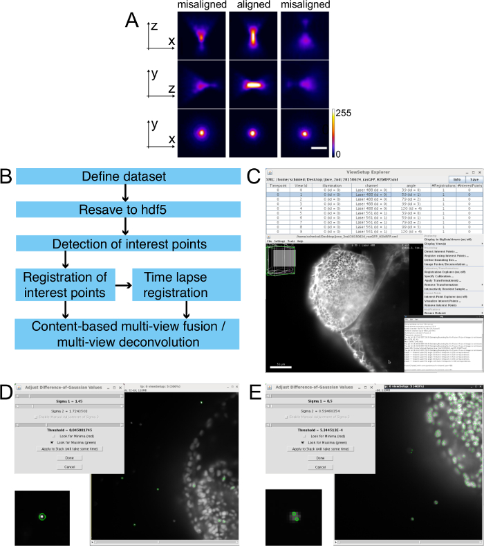
Figure 1: Multiview Reconstruction workflow and interest point detection. (A) Light sheet alignment based on fluorescent bead imaging. The system is aligned (center), when the bead image has a symmetrical hourglass shape in xz and yz projections. The examples of misaligned light sheet in either direction are shown on left and right. The maximum intensity projections of a 500 nm bead in xz, yz and xy axes are shown. Note that the ratio of intensity of the central peak of the Airy disc (in xy) to the side lobes is greater, when the lightsheet is correctly aligned compared to the misaligned situation. Images were taken with 20X/1.0 W objective at 0.7 zoom. Scale bar represents 5 µm. (B) The dataset is defined and then resaved into the HDF5 format. The beads are segmented and then registered. For a time series each time point is registered onto a reference time point. The data are finally fused into a single isotropic volume. (C, top) The ViewSetup Explorer shows the different time points, angles, channels and illumination sides of the dataset. (C, left lower corner) The BigDataViewer window shows the view that is selected in the ViewSetup Explorer. (C, middle right) Right click into the ViewSetup Explorer opens the processing options. (C, right lower corner) The progress and the results of the processing are displayed in the log file. (D and E) The aim of the detection is to segment as many interest points (beads) with as little detection in the sample as possible here shown as screenshots from the interactive bead segmentation. (D and E, upper left corner) The segmentation is defined by two parameters, the Difference-of-Gaussian Values for Sigma 1 and the Threshold. (D) An example of a successful detection with a magnified view of a correctly detected bead. (E) Segmentation with too many false positives and multiple detections of a single bead. Scale bar in (C) represents 50 µm. Please click here to view a larger version of this figure.

3. Resave Dataset in HDF5 Format
   1. To resave the entire dataset, select all the files with Ctrl/Apple+a and right click. Then select resave dataset and as HDF5.
   2. A window will appear displaying a warning that all views of the current dataset will be resaved. Press yes.
      NOTE: The program will continue to resave the .czi files to hdf5 by opening every file and resaving the different resolution levels of the hdf5 format. It will confirm with 'done' upon completion. Resaving usually takes a few min per timepoint (see Table 1).
      NOTE: Since the files in the hdf5 format can be loaded very fast, it is now possible to view the unregistered dataset by 'right click' into the explorer and toggling 'display in BigDataViewer (on/off)'. A BigDataViewer window will appear with the selected view (Figure 1C). The core functions of the BigDataViewer³³ are explained in Table 2 and http://fiji.sc/BigDataViewer.
4. Detect Interest Points
   1. Select all time points with Ctrl/Apple+a and right click select detect interest points.
   2. Select Difference-of-Gaussian³⁴ for type of interest point detection. Since the bead-based registration is used here, type "beads" into the field for label interest points. Activate 'Downsample images prior to segmentation'.
   3. In the next window, observe the detection settings. For 'subpixel localization' use '3-dimensional quadratic fit'³⁴ and to determine the Difference-of-Gaussian values and radius for bead segmentation use 'interactive' in the i'nterest point specification'.
   4. For 'Downsample XY' use 'Match Z Resolution (less downsampling)' and for 'Downsample Z' use 1×. The z step size is bigger than the xy pixel size, thus simply down sampling the xy to match the z resolution is sufficient. Select 'compute on CPU (JAVA)'. Press 'OK'.
   5. In a pop up window, select one view for testing the parameters from the drop down menu. Once the view loads, adjust brightness and contrast of the window with Fiji > Image > Adjust > Brightness/Contrast or Ctrl + Shift + C. Tick the box 'look for maxima (green)' for bead detection.
   6. Observe the segmentation in the 'viewSetup' as green rings around the detections when looking for maxima and red for minima. The segmentation is defined by two parameters, the Difference-of-Gaussian Values for Sigma 1 and the Threshold (Figure 1D). Adjust them to segment as many beads around the sample and as few false positive detections within the sample as possible (Figure 1D). Detect each bead only once and not multiple times (Figure 1E). After determining the optimal parameters, press 'done'.
      NOTE: The detection starts by loading each individual view of the time point and segmenting the beads. In the log file, the program outputs the number of beads it detected per view. The detection should be done in a few seconds (see Table 1).
   7. Press save when the amount of detections is appropriate (600 to several thousand per view).
      NOTE: A folder will be created in the data directory, which will contain the information about the coordinates of the detected beads.
5. Register Using Interest Points
   1. Select all time points with Ctrl/Apple+a, right click and select 'Register using Interest Points'.
   2. Use 'fast 3d geometric hashing (rotation invariant)' for bead detection as 'registration algorithm'.
      NOTE: This algorithm assumes no prior knowledge about the orientation and positioning of the different views with respect to each other.
   3. For registration of the views onto each other, select 'register timepoints individually' as 'type of registration'. For 'interest points' in the selected channel, the previously specified label for the interest points should now be visible (i.e. "beads").
   4. In the next window, use the pre set values for registration. Fix the first view by selecting 'Fix tiles: Fix first tile and use Do not map back' (use this if tiles are not fixed) in the 'Map back tiles' section.
   5. Use an 'affine transformation model' with 'regularization'.
      NOTE: The allowed error for RANSAC will be 5px and the 'significance for a descriptor match' will be 10. For 'regularization' use a 'rigid model' with a lambda of 0.10, which means that the transformation is 10% rigid and 90% affine³⁵. Press OK to start the registration.
      NOTE: As displayed in the log window, first each view is matched with all the other views. Then the random sample consensus (RANSAC)³⁶ tests the correspondences and excludes false positives. For a robust registration, the RANSAC value should be higher than 90%. When a sufficient number of true candidates corresponding between two views are found, a transformation model is computed between each match with the average displacement in pixels. Then the iterative global optimization is carried out and all views are registered onto the fixed view. With successful registration, a transformation model is calculated and displayed with its scaling and the displacement in pixels. The average error should be optimally below 1 px and the scaling of the transformation close to 1. The registration is executed in seconds (see Table 1).
   6. Confirm that there is no shift between different views as observed on fine structures within the sample, e.g. cell membranes. Then save the transformation for each view into the .xml file.
      NOTE: Now the registered views are overlapping each other in the BigDataViewer (Figure 2A) and the bead images should be overlaying as well (Figure 2B).
   7. Remove the transformations by selecting the time points right click on them and then select Remove Transformations > Latest/Newest Transformation.

Figure 2: Results of the multiview reconstruction. (A) Overlaid registered views, each in a different color to demonstrate the overlap between them. (B) Magnified view showing the overlap of the PSFs of beads imaged from the different views. (C) Close up of a bead after fusion, the PSF is an average of the different views. (D) PSF of the same bead as in (C) after multiview deconvolution showing that the PSF collapses into a single point. (E) x-y section and (F) y-z section of a single view of an optic vesicle, in which membranes are labeled with GFP showing degradation of the signal in z deeper in the tissue. (G) x-y section and (H) y-z section of the same view after weighted-average fusion of 4 views approximately 20 degrees apart with slightly more degraded x-y resolution overall but increased z-resolution. (I) x-y section and (J) y-z section of the same data after multiview deconvolution, showing a significant increase in resolution and contrast of the signal both in xy and in z. Images in (E-J) are single optical slices. Scale bar represents 50 µm (A, B, E-J) and 10 µm (C, D). Please click here to view a larger version of this figure.

6. Time-lapse Registration
   1. Select the whole time lapse, right click and choose 'Register using Interest Points' to stabilize the time-lapse over time.
   2. In the 'Basic Registration Parameters window select Match against one reference time point (no global optimization) for Type of registration'. Keep the other settings the same as in the registration of the individual time points.
   3. In the next window, select the time point to be used as a reference, typically a time point in the middle of the time-lapse. Tick the box 'consider each timepoint as rigid unit', since the individual views within each time point are already registered onto each other.
   4. Tick the box for 'Show timeseries statistics'. The other registration parameters remain as before including the regularization. Press OK.
      NOTE: In the log window, the same output will be displayed as in the individual time point registration. If the registration for the individual time points was successful and robust, the RANSAC is now 99-100% and the average, minimum and maximum error is usually below 1 px. Save this registration before proceeding.

7. Multiview Fusion

NOTE: The resulting transformations from the registration steps are used to compute a fused isotropic stack out of the multiple views. This stack has increased number of z slices compared to the original data, because the z spacing is now equal to the original pixel size in xy. The fusion can be performed by either a content-based multiview fusion^21,31 or Bayesian-based multiview deconvolution³¹, which are both implemented in the multiview reconstruction application.

1. Bounding Box
   NOTE: Fusion is a computationally expensive process (see Table 1), thus reducing the amount of data by defining a bounding box significantly increases the speed of processing.
   1. Select all time points right click and choose Define 'Bounding Box'. Use 'Define with BigDataViewer' and choose a name for the bounding box.
   2. Move the slider for 'min' and 'max' in every axis to determine the region of interest and then press 'OK'. The parameters of the bounding box will be displayed.
      NOTE: The bounding box will contain everything within the green box that is overlaid with a transparent magenta layer.
2. Content-based Multiview Fusion
   NOTE: Content-based multiview fusion²¹ takes the image quality differences over the stack (i.e. degradation of the signal in z) into account and applies higher weights for better image quality instead of using a simple averaging.
   1. Select the time point(s) that should be fused in the 'ViewSetup Explorer', right click and select 'Image Fusion/Deconvolution'.
   2. In the Image Fusion window, select 'Weighted-average fusion' from the drop down menu, and choose 'Use pre-defined Bounding Box for Bounding Box'. For the output of the fused image select 'Append to current XML Project', which writes new hdf5 files to the already existing hdf5 files and allows using the registered unfused views and the fused image together. Press 'OK'.
   3. Then in the' Pre-define Bounding Box' pop up window select the name of the previously defined bounding box and press 'OK'.
   4. Observe the parameters of the bounding box in the next window. For quick fusion, apply a down sampling on the fused dataset.
      NOTE: If the fused stack is above a certain size, the program will recommend using a more memory efficient 'ImageLib2 containe'r. Switch from 'ArrayImg' to the 'PlanarImg (large images, easy to display) or CellImg (large images)' container, which allow processing of larger data. Otherwise use the predefined settings and apply 'blending and content-based fusion'. Proceed by pressing 'OK'.
   5. Observe the hdf5 settings in the next window. Use the predefined parameters and start the fusion process. Make sure that Fiji has assigned enough memory in Edit > Options > Memory & Threads.
3. Multiview Deconvolution
   NOTE: Multiview Deconvolution³¹ is another type of multiview fusion. Here additionally to the fusion, the PSF of the imaging system is taken into account in order to deconvolve the image and yield increased resolution and contrast of the signal (compared in Figure 2C-J, Figure 5 and Movie 3).
   1. Select the time point(s) to be deconvolved, right click and press 'Image Fusion/Deconvolution'.
   2. Select 'Multiview Deconvolution' and use 'the pre-defined bounding box and append to the current XML project'. Select the bounding box and continue.
      NOTE: The pre-defined parameters for the deconvolution are a good starting point. For the first trial use '20 iterations' and assess the impact of the deconvolution by using the 'Debug mode'. Finally set the compute on to in 512 x 512 x 512 blocks.
   3. In the next window, use the pre-defined settings. Set the 'debug mode' to display the results every '5 iterations'.
      NOTE: The output of the deconvolution is 32-bit data, however the BigDataViewer currently only supports 16-bit data. In order to append the output of the deconvolution to the existing hdf5 dataset, it has to be converted to 16-bit.
   4. For the conversion, run 'Use min/max of the first image (might saturate intensities over time)'.
      NOTE: The deconvolution will then start by loading the images and preparing them for the deconvolution.
4. BigDataServer
   1. In order to share the very large XML/HDF5 datasets use the http server BigDataServer³³. An introduction to how to setup and connect to such server can be found at http://fiji.sc/BigDataServer.
   2. To connect to an existing BigDataServer open Fiji > Plugins > BigDataViewer > BrowseBigDataServer.
   3. Enter the URL including the port into the window.
      NOTE: The movies described in this publication are accessible via this address: http://opticcup.mpi-cbg.de:8085
   4. Observe a window that allows selecting the available movies. Double click to open the BigDataViewer window and view the data as described previously.

Supplementary: Checklist of Material Needed Before Starting

• zebrafish embryos/larvae expressing fluorescent proteins (Keep the embryos in the zebrafish E3 medium without methylene blue. For stages older than 24 hr counteract the pigmentation by adding PTU to a final concentration of 0.2 mM.)
• fluorescent stereoscope
• capillaries (20 μl volume, with a black mark) and appropriate plungers (Do not reuse the capillaries. The plungers, on the other hand, can be reused for several experiments.)
• 1.5 ml plastic tubes
• sharp tweezers
• glass (fire polished) or plastic pipettes (plastic can be used for 24 hr and older embryos)
• glass or plastic dishes diameter 60 mm (plastic can be used for 24 hr and older embryos)
• two 100 ml beakers
• 50 ml Luer-Lock syringe with 150 cm extension hose for infusion (The hose and syringe should be kept completely dry in between experiments to avoid contamination by microorganisms.)
• plasticine
• low melting point (LMP) agarose
• E3 medium (5 mM NaCl, 0.17 mM KCl, 0.33 mM CaCl₂, 0.33 mM MgSO₄)
• MS-222 (Tricaine)
• phenylthiourea (PTU)
• fluorescent microspheres (here referred to as beads)
• double distilled H₂O (ddH₂O)

Results

LSFM is an ideal method for imaging developmental processes across scales. Several applications are compiled here showing both short and long-term imaging of intracellular structures, as well as cells and entire tissues. These examples also demonstrate that LSFM is a useful tool at various stages of eye development from optic cup formation to neurogenesis in the retina. Movie 1 serves as an illustration of the general LSFM approach, first showing a zoomed out view of an intact embryo in the embedding agarose cylinder in brightfield and later showing a detailed view of the retina in the fluorescence channel.

Movie 1: LSFM of the zebrafish retina. To illustrate the LSFM approach, this movie shows first in the brightfield that the embryo is imaged intact inside the agarose cylinder before switching to fluorescence. Later it is shown that the big field of view enables observation of the whole retina. Next, the movie shows a magnified small region of the retina to highlight the good subcellular resolution. An Ath5:gap-GFP³⁷ transgenic zebrafish embryo was used for imaging. This transgene labels different neurons in the retina (mainly ganglion cells and photoreceptor precursors). The fluorescence part of the movie was captured as a single view recording with dual sided illumination using the 40X/1.0 W objective with 5 min intervals. The maximum intensity projection of a 30 µm thick volume is shown. Please click here to download this file.

Movie 2 demonstrates, how very fast intracellular events can be captured with high resolution; in this case the growth of microtubules at their plus ends in the retinal neuronal progenitor cells. The information contained in the movie allows for tracking and quantification of microtubule plus end growth.

Movie 2: Microtubule dynamics in a single cell. This movie captures growing plus tips of microtubules labeled by the plus tip marker protein EB3-GFP³⁸. The protein is expressed in a single retinal progenitor cell. The microtubules are growing predominantly in the direction from apical to basal (top to bottom). The average speed of the EB3 comets was measured as 0.28 ±0.05 µm/sec. The bright spot at the apical side of the cell exhibiting high microtubule nucleation activity is the centrosome. The wild type embryo was injected with hsp70:EB3-GFP plasmid DNA. The movie was acquired 4 hr after heat shock (15 min at 37 °C) at around 28 hrpost fertilization (hpf) as a single view recording with single sided illumination using the 63X/1.0 W objective and 1 sec time intervals. The single cell was cropped from a field of view covering the majority of the retina. The maximum intensity projection of two slices is shown. Please click here to download this file.

Figure 3 shows, how intracellular structures can be followed over many hours. Here, the centrosome within translocating retinal ganglion cells (RGCs) is captured.

Figure 3: Centrosome localization during the retinal ganglion cell translocation. This montage of a time-lapse experiment shows the position of the centrosome throughout the retinal ganglion cell (RGC) maturation. In the neuronal progenitors the centrosome is localized in the very tip of the apical process (1:00). During cell division, the two centrosomes serve as poles for the mitotic spindle (2:25). This division results in one daughter cell that differentiates into an RGC and a second daughter cell that becomes a photoreceptor cell precursor. After division, the cell body of the RGC translocates to the basal side of the retina, while the apical process remains attached at the apical side. Once the RGC reaches the basal side, its apical process detaches and the centrosome travels with it (6:15). The centrosome can be followed while gradually retracting together with the apical process (6:50, 7:20, 8:10). In the last frame (8:55) the ganglion cell is growing an axon from its basal side, while the centrosome is still localized apically. The mosaic expression was achieved by plasmid DNA injection into wild type embryo at one cell stage. The cells are visualized by the Ath5:GFP-caax (green) construct, which labels RGCs and other neurons. The centrosomes (arrowheads) are labeled by Centrin-tdTomato²⁹ expression (magenta). The apical side of the retina is at the top of the image and the basal side at the bottom. The maximum intensity projection of a 30 µm thick volume is shown. The images were cropped from a movie covering the whole retina. The movie starts at around 34 hr post fertilization (hpf). A z stack was acquired every 5 min with the 40X/1.0 W objective. Time is shown in hh:mm. Scale bar represents 10 µm. Please click here to view a larger version of this figure.

In Figure 4 it is displayed, how single cell behavior can be extracted from data capturing the whole tissue such as in Movie 1. Translocation of an RGC can be easily tracked and its apical and basal processes followed.

Figure 4: Translocation of a single retinal ganglion cell. The RGC translocation from apical to basal side of the retina occurs after the terminal mitosis as described in Figure 3. The RGC is labeled by expression of the Ath5:gap-GFP³⁷ transgene. The maximum intensity projection of a 30 µm thick volume is shown. The images were cropped from a movie covering the whole retina. The movie starts at around 34 hpf. A z stack was acquired every 5 min with the 40X/1.0 W objective. Time is shown in hh:mm. Scale bar represents 5 µm. Please click here to view a larger version of this figure.

Figure 5 demonstrates the ability of multiview LSFM to capture tissue scale morphogenetic processes with cellular resolution on the example of optic cup morphogenesis, during which optic vesicle transforms into an optic cup. The image quality can be vastly improved by multiview imaging, when the final image is combined from the information out of 5 different views (in this case) into one z stack with isotropic resolution. This figure illustrates the improvement in image quality after weighted-average fusion and further gain in image contrast and resolution after multiview deconvolution. The figure shows two optical slices in different orientations through the dataset. Additionally, a montage from the deconvolved dataset shows the optic cup morphogenesis over time. All the time points are then shown in Movie 3.

Figure 5: Comparison of image quality between single view and two methods of multiview fusion. (A) One optical slice of single view data shown from lateral view and (B) dorsal view. Stripe artifacts and degradation of the signal deeper inside the sample are apparent. Also a part of the image visible in the fused data (C-F) was not captured in this particular view. (C) The same optical slice, now as multiview fused data shown from lateral view and (D) dorsal view. Note that stripe artifacts are suppressed and structures deep in the sample are better resolved. (E) The same optical slice now as multiview deconvolved data shown from lateral view and (F) dorsal view. Note the increased contrast and resolution so the individual cell membranes and nuclei can be well distinguished. The resolution does not deteriorate notably deeper inside the sample. The dataset was acquired with dual sided illumination from 5 views approximately 20 degrees apart. The z stacks of about 100 µm with 1.5 µm step size were acquired at each view in 10 min intervals for 10 hours with the 20X/1.0 W objective. Input images for the multiview fusion and deconvolution were down sampled 2× to speed up the image processing. 15 iterations of the multiview deconvolution were run. (G) The montage shows a cropped area of the dorsal view from the deconvolved data to highlight the morphogenetic events during early eye development from the optic vesicle to the optic cup stage. The two layers of the optic vesicle, which are initially similar columnar epithelia, differentiate into distinct cell populations. The distal layer close to the epidermis becomes the retinal neuroepithelium (RN) and the proximal layer close to the neural tube becomes the retinal pigment epithelium (RP). The cells in the RN elongate and invaginate to form the optic cup (1:40 to 5:00); at the same time the RP cells flatten. The surface ectoderm is induced to form a lens (1:40), which invaginates later (5:00). The movie starts at 17 hpf. Time is shown in hh:mm. All the cellular membranes are labeled by the β-actin:ras-GFP transgene and all the nuclei are labeled by the hsp70:H2B-RFP transgene. Scale bar represents 30 µm. FB forebrain, LE lens, OP olfactory placode, RN retinal neuroepithelium, RP retinal pigment epithelium. Please click here to view a larger version of this figure.

Movie 3: Optic cup morphogenesis shown with single view and two methods of multiview fusion. The time-lapse movie illustrates the complete process of optic cup morphogenesis from the optic vesicle to the optic cup stage. It shows a single optical slice from the lateral view (top) and a single optical slice from the dorsal view (bottom). The cells of the developing optic vesicle undergo complex rearrangements to finally form the hemispherical optic cup with the inner retinal neuroepithelium and outer retinal pigment epithelium. A lens is formed from the surface ectoderm. It invaginates along with the neuroepithelium and sits in the optic cup. All cellular membranes are labeled by expression of the β-actin:ras-GFP (green) transgene and the nuclei are labeled with hsp70:H2B-RFP (magenta). The movie starts at around 17 hpf. The dataset was acquired with dual sided illumination from 5 views approximately 20 degrees apart and a z stacks of about 100 µm were acquired every 10 min with the 20X/1.0 W objective. Time is shown in hh:mm. Scale bar represents 50 µm. Please click here to download this file.

Discussion

1. Critical steps and troubleshooting for the data acquisition

The typical imaging settings for a GFP and RFP expressing sample can be found in Table 3. In the described microscope setup the light sheet is static, formed by a cylindrical lens. The two illumination objectives are air lenses and the detection objective is a water-dipping lens. Zoom 1.0 with 20X/1.0 or 40X/1.0 objectives gives 230 nm and 115 nm pixel size and a field of view of 441 x 441 µm or 221 x 221 µm respectively. It is recommended to use the default light sheet thickness with center to border ratio 1:2. For 20X/1.0 this thickness corresponds to 4.5 µm and for 40X/1.0 to 3.2 µm in the center. If imaging speed is not the primary priority, use separate tracks in case of a multicolor sample to avoid the crosstalk of fluorescence emission between the channels. The highest speed of acquisition is limited to 50 msec per z step by the speed of movement of the z-driver. If the goal is to achieve the maximum imaging speed in case of, e.g., two tracks with dual sided illumination, the exposure time must be set so that the sum of all the images taken per z step is below 50 msec. On the other hand, if only a single image is acquired per z step, it is not beneficial to set the exposure time shorter than 50 msec.

1920 x 1920 image size

16-bit

Pivot scan on

Dual sided illumination with online fusion

10X/0.2 illumination objective

20X/1.0 W Plan-Apochromat detection objective

Track 1: Excitation 488 nm typically 2% of 100 mW laser, 550 nm SP emission filter

Track 2: Excitation 561 nm typically 3% of 75 mW laser, 585 nm LP emission filter

Exposure time up to 100 msec

Z stack thickness 50-100 μm

1-1.5 μm z step size in the continuous z drive mode

Incubation at 28.5 °C

Table 3: Imaging Settings.

Inspecting the sample after the experiment

It is important to ensure that the specimen is still healthy at the end of the experiment. As a first readout, check the heartbeat of the specimen under a stereoscope. With a pair of sharp forceps the sample can be taken out of the agarose and moved to the incubator to develop further in order to check if it was affected by the imaging. Alternatively, it can be fixed for antibody staining.

Mounting and drift

It is essential to keep the osmolarity of the chamber solution close to the osmolarity of the embedding agarose, otherwise swelling/shrinking of the agarose and subsequent instability of the sample will occur. Therefore, use the same solution (E3 medium without methylene blue) to fill the chamber and to prepare the 1% low melting point agarose aliquots. Additionally, do not leave the agarose in the 70 °C heating block for more than 2 hr, as it can lose its gelling properties.

Do not embed the fish into too hot agarose, as this can lead to heat shock response or death of the embryo. If unsure about the effect of warm agarose on the embryos, check that the tail does not bend and that the heart rate does not slow down. If this occurs, use a different embryo for the experiment.

Keep the overall length of the agarose column with the sample short (around 2 cm) and mount the zebrafish with its head oriented towards the plunger tip. Likewise, the agarose cylinder extruded from the capillary should be kept as short as possible. These measures will ensure stability of the sample throughout the movie. At the same time, the agarose column must be long enough so that the glass capillary itself does not reach into the light path, as this would cause major refraction and reflection.

The initial drift of the sample is caused by the volume changes of the agarose cylinder itself. Sliding of the plunger is not the reason for it. Therefore, it does not help to fix the plunger with plasticine or nail polish. The embryo might change its position during the movie due to its natural growth too. Accordingly, it is advisable to center the region of interest in the middle of the field of view and keep some room at the edges to accommodate these movements.

Reduced amount of embedding medium in the light path

Orienting the sample correctly helps to achieve the best possible image quality¹⁵. Generally, excitation and emission light should travel through as little tissue and mounting media as possible. The optimal solution is agarose-free mounting. This was achieved for example in a setup for Arabidopsis lateral root imaging¹⁴, in which the main root was mounted into phytagel and the lateral roots were subsequently let to grow out of the gel column completely. Agarose-free mounting was also developed for imaging of the complete embryogenesis of Tribolium beetle over two days¹². Image quality improvement was not a primary motivation in that case. Tribolium embryos simply do not survive inside the agarose long enough. An absolutely embedding media-free mounting has not been achieved for long term imaging in zebrafish. Still, we can take advantage of the fact that when the agarose solidifies, most embryos are positioned diagonally in the capillary with one eye located deep in the agarose and the second eye being close to the surface of the embedding column. The eye closer to the surface provides superior image quality and therefore should be imaged preferentially.

Agarose concentration and long-term imaging

The concentration of agarose for mounting is a compromise between stability of the sample and the possibility to accommodate growth of the embryo and diffusion of oxygen to it. There is no additional gain in the stability of the sample when using agarose concentrations higher than 1%. As a starting point for optimizing the experiments we recommend 0.6% agarose, which is also suitable for embryos younger than 24 hpf that are too delicate to be mounted into 1% agarose. To anaesthetize older embryos and larvae, the MS-222 concentration can be raised to 200 µg/ml without side effects¹³.

In case developing embryos are imaged for longer than ±12 hr, agarose mounting is not recommended, because it restricts the growth of the embryo and causes tail deformation. This issue was solved for zebrafish by mounting embryos into FEP polymer tubes with refractive index similar to water^13,39. Mouse embryos, on the other hand, can be immobilized in hollow agarose cylinders⁴⁰ or in holes of an acrylic rod attached to a syringe⁴¹. FEP tube mounting is not recommended as default method though, because the wall of the tube refracts the light slightly more than agarose.

Light sheet alignment

For good image quality it is critical to perform the automatic light sheet alignment before every experiment. Especially if the zoom settings were changed, the objectives were taken out, or a different liquid was used in the chamber.

Illumination

The pivot scanning of the light sheet should always be activated. For large scattering specimens, it is necessary to apply the dual sided illumination with online fusion to achieve even illumination across the field of view. Dual sided illumination also diminishes a specific problem of the eye imaging, which is the refraction of the incoming light sheet by the lens of the embryo. Smaller, less scattering specimens can be efficiently imaged using single sided illumination, which shortens the imaging time by half and can result in slightly better image quality compared to dual sided illumination. This is because the light paths for the two illumination arms are always different and the more efficient one can be chosen. Additionally, the two light sheets coming from each side are never perfectly in one plane, which causes mild blurring after the fusion. For very fast intracellular events, like the growing microtubules (Movie 2), the dual sided illumination is not appropriate, since the images with illumination from left and right are acquired sequentially, which could result in motion blur.

Photobleaching and phototoxicity

Less fluorophore photobleaching is often mentioned as a major advantage of the LSFM. We would argue that the aim should be no photobleaching at all. If there is noticeable photobleaching in the live imaging experiment, the specimen is probably already out of its physiological range of tolerated laser exposure. When imaging the zebrafish embryos in the spinning disc microscope, in our experience, high phototoxicity can stall embryo development even before the fluorescent signal bleaches markedly. Therefore, the imaging settings in the LSFM should be adjusted so that little or no photobleaching is observed. Even though LSFM is gentle to the sample, it is prudent to use only as much laser power and exposure time as needed to achieve a signal to noise ratio sufficient for the subsequent data analysis.

Z-stack, time intervals and data size

The files generated by LSFM are usually very large; sometimes in the terabyte range. It is often necessary to make a compromise between image quality and data size. This is particularly the case for z spacing of stacks and intervals in the time-lapse acquisitions. To define the z intervals, the Optimal button in the Z-stack tool tab should ideally be used, especially if the dataset will be deconvolved later. It calculates the spacing to achieve 50% overlap between neighboring optical slices. Still, somewhat larger z intervals are usually acceptable. They reduce the time needed to acquire the z stack as well as the final file size. The optimal time sampling depends on the process of interest. For overall eye development 5-10 min intervals are usually acceptable. If some structures are to be automatically tracked, the subsequent time points must be sufficiently similar.

Fluorescent beads

Fluorescent beads primarily serve as fiducial markers for registering different views of a multiview dataset onto each other. Always vortex the bead solutions thoroughly before use. Do not heat the beads as this can lead to loss of the fluorescent dye. The optimal bead concentration for the multiview registration has to be determined experimentally. The described plugin works best with around 1,000 detected beads throughout each view. Larger (500 nm or 1,000 nm) beads are detected more robustly than smaller (less than 500 nm) beads. This is because larger beads are brighter and are easier to segment without false positive detections of structures in the sample. The disadvantage of the larger beads is that they are very prominent in the final fused and deconvolved image. For each new fluorescent marker, the appropriate bead size and fluorescence emission have to be optimized. To give an example of sample from Figure 5 and Movie 3, 100 nm green emission beads gave too many false positive detections in the membrane-GFP channel, but 1,000 nm red emission beads were robustly detected in the H2B-RFP channel with very few positive detections inside the sample. If the bead detection fails in the channel with the fluorescent marker, a separate channel only containing beads can be acquired, but this is not very practical. The sub-resolution sized beads give a direct readout of the point spread function (PSF) of the microscope, which can be used for deconvolution (Figure 2C-D). If registration and fusion works better with bigger beads (e.g. 1,000 nm), a separate image of the PSF can be acquired with sub-resolution, e.g., 100 nm beads. Using multicolor beads is helpful during registration of multichannel acquisition and for verifying that the channels overlay perfectly.

Addition of fluorescent beads is not necessary when imaging from a single view without subsequent multiview registration and fusion. However, even in those cases beads can be helpful during the initial light sheet adjustment to check for the quality of the light sheet and in general to reveal optical aberrations. Such optical aberrations may originate from various sources like damaged or dirty objectives, dirty windows of the chamber or inhomogeneity in the agarose. Beads can also be used for drift correction by the multiview registration Fiji plugin²⁰.

Multiview

For the multiview reconstruction purpose, it is better to acquire an odd number of views 3, 5 and so on, which are not opposing each other. This improves deconvolution since the PSFs are imaged from different directions. It is also important to confirm at the beginning of the time lapse acquisition that there is sufficient overlap among the views. This is best done empirically, i.e., immediately confirming that the views in the first time point can be successfully registered. When the goal of the multiview acquisition is to increase the resolution of an image of a large scattering specimen, it is not advisable to image the entire specimen in each view, but to stop around the center of the sample, where the signal deteriorates. The low quality acquisition from the second half of the specimen would not add useful information to the multiview reconstruction.

2. Critical steps and troubleshooting for the data processing

Currently, there exist several possibilities for processing multiview data from a light sheet microscope that are well documented and relatively easy to adopt. We use the multiview reconstruction application, which is an open source software implemented in Fiji³² (Stephan Preibisch unpublished, Link 1a and Link1b in the List of Materials). This plugin is a major redesign of the previous SPIM registration plugin²⁰, reviewed by Schmied et al.⁴², integrating the BigDataViewer and its XML and HDF5 format³³ with the SPIM registration workflow (Figure 1B, Link 2, Link 3). This application can be also adapted for high performance computing cluster, which significantly speeds up the processing⁴³. This multiview registration application is actively developed further and keeps improving. In case of problems or features requests for the described software, please file issues on the respective GitHub pages (Link 4 for Multiview Reconstruction and Link 5 for BigDataViewer).

The second option is to use the commercial software available together with the microscope. This solution works well and employs the same principle of using fluorescent beads to register the different views. However, it lacks the option to visualize the whole dataset fast like with the BigDataViewer. Also the software cannot be adapted to the cluster and furthermore the processing blocks the microscope for other users, unless additional license for the software is purchased.

The third option, which is also an open source software, was recently published by the Keller lab⁴⁴ and provides a comprehensive framework for processing and downstream analysis of the light sheet data. This software is using information from within the sample to perform multiview fusion, therefore it does not require the presence of fluorescent beads around the sample. But at the same time it assumes orthogonal orientation of the imaging views (objectives), so it cannot be used for data acquired from arbitrary angles⁴⁴.

Hardware requirements

The hardware used for processing can be found in Table 4. There has to be enough storage capacity and a clear pipeline for data processing available, ahead of the actual experiment. Acquisition of the images is faster than subsequent analysis and it is easy to get flooded with unprocessed data. It is often unrealistic to store all the raw images, but rather a cropped version or processed images like fused views, maximum intensity projections or spherical projections⁴⁵.

Processor	Two Intel Xeon Processor E5-2630 (Six Core, 2.30 GHz Turbo, 15 MB, 7.2 GT/sec)
Memory	128 GB (16×8 GB) 1600 MHz DDR3 ECC RDIMM
Hard Drive	4×4 TB 3.5inch Serial ATA (7.200 rpm) Hard Drive
HDD Controller	PERC H310 SATA/SAS Controller for Dell Precision
HDD Configuration	C1 SATA 3.5 inch, 1-4 Hard Drives
Graphics	Dual 2 GB NVIDIA Quadro 4000 (2 cards w/ 2 DP & 1 DVI-I each) (2 DP-DVI & 2 DVI-VGA adapter) (MRGA17H)
Network	Intel X520-T2 Dual Port 10 GbE Network Interface Card

Table 4: Hardware Requirements.

Data processing speed

The time needed for data processing depends on the dimensions of the data and on the used hardware. In Table 1, we provide an overview of the time required for the key steps in processing an example 8.6 GB multiview dataset that consisted of 1 time point with 4 views and 2 channels.

Processing step	Time	Protocol step
Resave as HDF5	6 min 30 sec	6.3
Detect Interest Points	20 sec	6.4
Register using interest points	3 sec	6.5
Content-based multiview fusion	4 hr	7.2
Multiview deconvolution (CPU)	8 hr	7.3
Multiview deconvolution (GPU)	2 hr	7.3

Table 1: Data Processing Time.

Input data formats for multiview reconstruction

The Fiji Plugin Multiview Reconstruction can support .czi, .tif and ome.tiff formats. Due to the data structure of the .czi format, discontinuous datasets are not supported without pre-processing. Discontinuous means that the recording had to be restarted (e.g. to readjust the positions due to drift of the sample). In this case the .czi files need to be resaved as .tif. For .tif files each view and illumination direction needs to be saved as a separate file.

Calibration of pixel size

The microscope-operating software calculates the calibration for the xy pixel size based on the selected objective. However, the pixel size in z is defined independently by the step size. If a wrong objective is specified in the software the xy to z ratio is incorrect and the registration will fail.

Initial registration

After defining the dataset the number of registrations will be 1 and the number of interest points will be 0 in the ViewSetup Explorer. The initial registration represents the calibration of the dataset. Both the number of registrations and interest points will increase during processing.

Down sampling for detection of interest points

Using down sampling is recommended, since the loading of the files and the segmentation will be much faster. It is however important to note that the detection parameters will change depending on the down sampling, thus transferring detection settings between different down sample settings is not possible.

Detection of interest points

It is advisable to segment as many true beads as possible in each view, even at the price of obtaining some false positive detections, because they do not hinder the registration considerably. Spurious detections, if few in numbers, are excluded during registration (See Registration of interest points). However, massive false positive detections pose a problem to the algorithm. It not only reduces performance for the detection and the registration, since it takes much longer to segment the image as well as compare these beads between the views, but it also reduces the accuracy of the registration. This can be addressed by using more stringent detection parameters. Additionally, over segmentation of the beads (i.e. multiple detections on one bead Figure 1E) is detrimental to the registration and should be avoided.

Registration of interest points

To register the views onto each other, the location of each bead in each view is described by its position with respect to its three nearest neighboring beads. These constellations are forming a local geometric descriptor and allow comparing each bead between the views. Beads with matching descriptor between two views are then considered as candidate correspondences. Note that this works only for randomly distributed beads, for which the local descriptors are typically unique for each bead. One can use other structures such as nuclei in the sample for registration. However, in order to detect nuclei, which are distributed non randomly in the sample, other methods apply^20,21.

The candidate correspondences are then tested against RANSAC³⁶ in order to exclude false positives. Each correspondence is suggesting a transformation model for overlaying the views onto each other. True correspondences would likely agree on one transformation model, whereas outliers would each point to a different one. The true correspondences are then used to compute an affine transformation model between the two compared views. A global optimization with an iterative optimization algorithm is then carried out, during which all the views are registered onto the first view with the aim of minimal displacement between the views^20,21.

Time-lapse registration

Due to movement of the agarose and imprecise motor movement of the microscope stage, the position of each stack varies moderately over time. Whereas the registration of the individual time point removes the difference between the views of this time point, the time-lapse also needs to be registered as a whole. To this end, each individual time point is registered onto the reference time point.

Reference time point

If a time series with many time points is processed, a representative time point is selected as reference usually from the middle of the time series since the bead intensities can degrade over time due to bleaching. On this reference, the parameters for interest point detection, registration, bounding box and fusion can be determined. These parameters are then applied to the whole time lapse to compute a specific transformation model for each individual time point. During time-lapse registration all other time points are also registered spatially onto this reference time point. Thus the bounding box parameters for the entire recording are depending on this specific time point.

Multichannel registration

When imaging multiple channels, ideally the same fluorescent beads should be visible in all imaged channels. The detection and registration can then be performed on each channel individually, which takes into account the influence of the different light wavelengths on the transformation. Often this is not possible, because the beads are not visible in all channels or the beads are dominating the image too much in one channel and are too dim in the other channel(s). The typical solution is to use beads visible only in one channel for the detection and registration and the acquired transformation model (i.e. after detection, registration and time-lapse registration) is then applied to the other channels by Fiji > Plugins > Multiview Reconstruction > Batch Processing > Tools > Duplicate Transformations. In the drop down menu for Apply transformation of select One channel to other channels. In the following window select the XML and click OK. Then select the channel that contains the beads as Source channel and as Target channel select the channel(s) without beads. For Duplicate which transformations use Replace all transformations and press OK. The transformations are then copied to all other channels and saved in the XML. To see the new transformations in the ViewSetup Explorer, restart the MultiView Reconstruction Application.

Bounding box

The fusion of multiple views is computationally very intensive. However, large images are typically acquired to accommodate not only the sample, but also the beads around it. Once the registration parameters are extracted from the beads, they are no longer useful as part of the image. Therefore, to increase the efficiency of the fusion, only the parts of the image stacks containing the sample should be fused together. A region of interest (bounding box) should be defined to contain the sample and as little of the surrounding agarose as possible. For the example in Figure 2 a weighted average fusion on the entire volume with 2229×2136×2106 px would require 38,196 MB of RAM, whereas with a bounding box the volume is reduced to 1634×1746×1632 px and the memory requirements are reduced to 17,729 MB.

Content-based multiview fusion

The challenge in fusing multiview data is that the views usually end abruptly and do not contain the same image quality for the same voxels. Simple averaging of the views would therefore lead to blending artifacts and unnecessary image degradation. Content-based multiview fusion takes both of these problems into account. First, it blends the different views, where one image ends and the other one begins and second, it assesses the local image quality and applies higher weights to higher image quality in the fusion²¹. Compared to a single view there is an improvement of the resolution in z with a slight degradation of the signal in xy (Figure 2E-H, Figure 5A-D).

Multiview deconvolution

Multiview deconvolution is another approach to achieve the fusion of the views. With this method also the PSFs of the different views are taken into account in order to recover the image that has been convolved by the optics of the microscope. This method drastically improves image quality by removing image blur and increasing resolution and contrast of the signal³¹ (Figure 2C-D, Figure 2I-J, Figure 5E-G, Movie 3).

Deconvolution is computationally very intensive (see Table 1), thus using a GPU for processing increases the speed of this process. It may also be necessary to perform the deconvolution on down sampled data. To down sample, use Fiji > Multiview Reconstruction > Batch Processing > Tools > Apply Transformations. This will apply a new transformation model on the views that will be saved in the .xml file.

HDF5 file format for BigDataViewer and BigDataServer

The BigDataViewer³³ allows easy visualization of terabyte-sized data. How to control the BigDataViewer is summarized in Table 2. A screencast of the basic operation of the program is also available as a supplement in its original publication³³. The BigDataViewer is centered on an .xml file, which contains the metadata, and an hdf5 file, which contains the image data. The image data are present in the hdf5 in multiple resolution levels in 3D blocks. The multiple resolution levels allow for visualizing the data faster with lower resolution, before the full resolution is loaded. Individual blocks are only loaded into memory when needed. Thus, the hdf5 image format allows direct and fast visualization of the data via the BigDataViewer³³. It also speeds up processing since the loading of the files is carried out more efficiently. Therefore, we recommend resaving the dataset into this format, although it is not strictly required for the processing. For further explanation of the data format, please refer to Link 3. Additionally, the datasets can be shared with collaborators or the public using the BigDataServer³³ (Link 6).

key	effect
F1	shows the Help with a brief description of the BigDataViewer and its basic operation
< > or mouse wheel	movement in z
up and down arrow	zoom in and out
right click and drag	moves sample in the viewer
left click and drag	rotates sample around the cursor
slider at the bottom of the viewer or Tab and left or right arrow	moves on time axis
additionally pressing shift	faster movement or rotation along any axis
x and then left  and right arrow	rotates around the x axis
y and then left  and right arrow	rotates around the y axis
z and then left  and right arrow	rotates around the z axis
shift and x	orients the view along x axis
shift and y	orients the view along y axis
shift and z	orients the view along z axis
i	switches between the different interpolation modes (i.e. nearest neighbor and trilinear)
s or Settings > Brightness & Contrast	modifies the color of the channels, brightness and contrast
F6 or Settings > Visibility and grouping	changes the displayed groups, enables grouping to overlaying different groups and calling the groups via the number keys
F10 or Tools > Record Movie	acquires a time series of the currently displayed slice

Table 2: Big Data Viewer.

3. Limitations of the described implementation of LSFM

Low throughput

In a typical LSFM experiment only one sample per experiment is imaged. Still, in our experience, a lot of useful information can be extracted from that single sample. High throughput imaging of multiple embryos has been recently achieved in home built LSFM setups ^46-48, although typically at the expense of freedom of sample positioning and rotation.

Insufficient penetration deep into tissues

Even though zebrafish embryos are translucent, the obtained image quality is deteriorating quickly when imaging deeper in the tissue due to scattering and absorption. Partially this is an effect of scattering and absorption of the emitted fluorescence by the sample and cannot be corrected in the current setup. Another source of the uneven image quality is the irregular illumination. The light sheet is incident from the left or right side and any objects in its path refract it, which results in stripe artifacts and blur. The dual sided illumination and multiview fusion can diminish the artifacts in the final image. Lastly, the image quality tends to be slightly worse towards the margin of the field of view due to the natural geometry of the light sheet, which is becoming thicker towards the edges.

Limited chemical manipulation

The use of drugs or inhibitors is widespread in zebrafish research. In this microscope use of drugs is constrained, due to the big volume of the sample chamber and considerations of other users of the instrument, who share the same chamber. Using an extra chamber dedicated to drug experiments can solve this issue. Filling the chamber partially with glass beads reduces the volume of liquid that is required.

No photomanipulation

Currently there is no possibility of localized optical manipulation like photoconversion, or laser ablation in this microscope. Nevertheless, home built setups can be used for such specific applications.

4. Significance and future applications

LSFM is the best method available to date for fast imaging of big volumes of live embryos. Most of the experiments conceivable on a confocal microscope can also be performed on a light sheet microscope with aforementioned advantages. In the case of imaging of eye development, the speed of LSFM is not the crucial parameter. Instead, the low phototoxicity and flexibility in sample positioning are the decisive benefits.

The LSFM data have a high SNR, which helps to achieve good deconvolution results and is also beneficial for automated image analysis and object tracking. In conclusion, LSFM is a great tool for generating quantifiable data on embryonic development and overall cell and tissue characteristics for subsequent modeling and physical descriptions of the processes in question.

Materials

List of materials used in this article

Name	Company	Catalog Number	Comments
Lightsheet Z.1 microscope	Carl Zeiss Microscopy
Low melting point agarose	Roth	6351.1
Low melting point agarose	Sigma	A4018 or A9414
Ethyl 3-aminobenzoate methanesulfonate (MESAB/MS-222/Tricaine)	Sigma	E10521
N-Phenylthiourea (PTU)	Sigma	P7629
500 nm red fluorescent beads F-Y 050	Millipore (Estapor)	80380495
20 μl (1 mm inner diameter, marked black) capilllaries	Brand	701904	sold as spare part for transferpettor
Teflon tip plungers for 20 μl capillaries	Brand	701932	sold as spare part for transferpettor
Circular glass coverslips diameter 18 mm, selected thickness 0.17 mm	Thermo scientific (Menzel-Glaser)
O-rings for chamber windows 17×1.5 mm	Carl Zeiss Microscopy
Tweezers, style 55	Dumont	0209-55-PO
50 ml Luer-Lock syringes	Becton Dickinson	300865
150 cm extension cable for infusion compatible with Luer-Lock syringes	Becton Dickinson	397400
Links
Link 1 Multiview reconstruction application			https://github.com/bigdataviewer/SPIM_Registration http://fiji.sc/Multiview-Reconstruction
Link 2 BigDataViewer			https://github.com/bigdataviewer
Link 3 BigDataViewer			http://fiji.sc/BigDataViewer
Link 4 Multiview reconstruction application-issues			https://github.com/bigdataviewer/SPIM_Registration/issues
Link 5 BigDataViewer-issues			https://github.com/bigdataviewer/bigdataviewer_fiji/issues
Link 6 BigDataServer			http://fiji.sc/BigDataServer

References

- Pantazis, P., Supatto, W. Advances in whole-embryo imaging: a quantitative transition is underway. Nat Rev Mol Cell Biol. 15 (5), 327-339 (2014).
- Truong, T. V., Supatto, W. Toward high-content/high-throughput imaging and analysis of embryonic morphogenesis. Genesis. 49 (7), 555-569 (2011).
- Keller, P. J. Imaging Morphogenesis: Technological Advances and Biological Insights. Science. 340 (6137), 1234168-1234168 (2013).
- Huisken, J., Swoger, J., Del Bene, F., Wittbrodt, J., Stelzer, E. H. K. Optical Sectioning Deep Inside Live Embryos by Selective Plane Illumination Microscopy. Science. 305 (5686), 1007-1009 (2004).
- Voie, A. H., Burns, D. H., Spelman, F. A. Orthogonal-plane fluorescence optical sectioning: three-dimensional imaging of macroscopic biological specimens. J Microsc. 170 (Pt 3), 229-236 (1993).
- Jemielita, M., Taormina, M. J., DeLaurier, A., Kimmel, C. B., Parthasarathy, R. Comparing phototoxicity during the development of a zebrafish craniofacial bone using confocal and light sheet fluorescence microscopy techniques. J Biophoton. 6 (11-12), 920-928 (2012).
- Stelzer, E. H. K. Light-sheet fluorescence microscopy for quantitative biology. Nat Meth. 12 (1), 23-26 (2015).
- Chen, B. C., Legant, W. R., et al. Lattice light-sheet microscopy: Imaging molecules to embryos at high spatiotemporal resolution. Science. 346 (6208), 1257998-1257998 (2014).
- Keller, P. J., Ahrens, M. B. Visualizing Whole-Brain Activity and Development at the Single-Cell Level Using Light-Sheet Microscopy. Neuron. 85 (3), 462-483 (2015).
- Pampaloni, F., Chang, B. -J., Stelzer, E. H. K. Light sheet-based fluorescence microscopy (LSFM) for the quantitative imaging of cells and tissues. Cell Tissue Res. 360 (1), 129-141 (2015).
- Weber, M., Mickoleit, M., Huisken, J. Light sheet microscopy. Quantitative Imaging in Cell Biology. , Elsevier Inc. 193-215 (2014).
- Strobl, F., Stelzer, E. H. K. Non-invasive long-term fluorescence live imaging of Tribolium castaneum embryos. Development. 141 (11), 2361-2361 (2014).
- Kaufmann, A., Mickoleit, M., Weber, M., Huisken, J. Multilayer mounting enables long-term imaging of zebrafish development in a light sheet microscope. Development. 139 (17), 3242-3247 (2012).
- Maizel, A., von Wangenheim, D., Federici, F., Haseloff, J., Stelzer, E. H. K. High-resolution live imaging of plant growth in near physiological bright conditions using light sheet fluorescence microscopy. Plant J. 68 (2), 377-385 (2011).
- Swoger, J., Muzzopappa, M., Lòpez-Schier, H., Sharpe, J. 4D retrospective lineage tracing using SPIM for zebrafish organogenesis studies. J Biophoton. 4 (1-2), 122-134 (2010).
- Keller, P. J., Schmidt, A. D., Wittbrodt, J., Stelzer, E. H. K. Reconstruction of zebrafish early embryonic development by scanned light sheet microscopy. Science. 322 (5904), 1065-1069 (2008).
- Wu, Y., Ghitani, A., et al. Inverted selective plane illumination microscopy (iSPIM) enables coupled cell identity lineaging and neurodevelopmental imaging in Caenorhabditis elegans. Proc Natl Acad Sci USA. 108 (43), 17708-17713 (2011).
- Sarov, M., Barz, C., et al. A genome-wide resource for the analysis of protein localisation in Drosophila. bioRxiv. , 028308(2015).
- Amat, F., Lemon, W., et al. Fast, accurate reconstruction of cell lineages from large-scale fluorescence microscopy data. Nat Meth. 11 (9), 951-958 (2014).
- Preibisch, S., Saalfeld, S., Schindelin, J., Tomancak, P. Software for bead-based registration of selective plane illumination microscopy data. Nat Meth. 7 (6), 418-419 (2010).
- Preibisch, S., Rohlfing, T., Hasak, M. P., Tomancak, P. Mosaicing of single plane illumination microscopy images using groupwise registration and fast content-based image fusion. SPIEMed Imaging. 6914, 69140E(2008).
- Reynaud, E. G., Peychl, J., Huisken, J., Tomancak, P. Guide to light-sheet microscopy for adventurous biologists. Nat Meth. 12 (1), 30-34 (2015).
- Keller, P. J., Schmidt, A. D., Wittbrodt, J., Stelzer, E. H. K. Digital Scanned Laser Light-Sheet Fluorescence Microscopy (DSLM) of Zebrafish and Drosophila Embryonic Development. Cold Spring Harb Protoc. 2011 (10), (2011).
- Pinto-Teixeira, F., Muzzopappa, M., Swoger, J., Mineo, A., Sharpe, J., Lòpez-Schier, H. Intravital imaging of hair-cell development and regeneration in the zebrafish. Front Neuroanat. , (2013).
- Keller, P. J. In vivo imaging of zebrafish embryogenesis. METHODS. , 1-11 (2013).
- Pitrone, P. G., Schindelin, J., et al. OpenSPIM: an open-access light-sheet microscopy platform. Nat Meth. 10 (7), 598-599 (2013).
- Gualda, E. J., Vale, T., Almada, P., Feijò, J. A., Martins, G. G., Moreno, N. OpenSpinMicroscopy: an open-source integrated microscopy platform. Nat Meth. 10 (7), 599-600 (2013).
- Martinez-Morales, J. R., Rembold, M., et al. ojoplano-mediated basal constriction is essential for optic cup morphogenesis. Development. 136 (13), 2165-2175 (2009).
- Strzyz, P. J., Lee, H. O., Sidhaye, J., Weber, I. P., Leung, L. C., Norden, C. Interkinetic Nuclear Migration Is Centrosome Independent and Ensures Apical Cell Division to Maintain Tissue Integrity. Dev Cell. 32 (2), 203-219 (2015).
- Young, L. K., Jarrin, M., Saunter, C. D., Quinlan, R., Girkin, J. M. Using SPIM to track the development of the focal power of the zebrafish lens. SPIE BiOS. 9334, 933408(2015).
- Preibisch, S., Amat, F., et al. Efficient Bayesian-based multiview deconvolution. Nat Meth. 11 (6), 645-648 (2014).
- Schindelin, J., Arganda-Carreras, I., et al. Fiji: an open-source platform for biological-image analysis. Nat Meth. 9 (7), 676-682 (2012).
- Pietzsch, T., Saalfeld, S., Preibisch, S., Tomancak, P. BigDataViewer: visualization and processing for large image data sets. Nat Meth. 12 (6), 481-483 (2015).
- Brown, M., Lowe, D. G. Invariant Features from Interest Point Groups. Proceedings of the British Machine Vision Conference. , BMVA Press. 23.1-23.10 (2002).
- Saalfeld, S., Fetter, R., Cardona, A., Tomancak, P. Elastic volume reconstruction from series of ultra-thin microscopy sections. Nat Meth. 9 (7), 717-720 (2012).
- Fischler, M. A., Bolles, R. C. Random sample consensus: a paradigm for model fitting with applications to image analysis and automated cartography. Commun ACM. 24 (6), 381-395 (1981).
- Zolessi, F. R., Poggi, L., Wilkinson, C. J., Chien, C. -B., Harris, W. A. Polarization and orientation of retinal ganglion cells in vivo. Neural Dev. 1 (1), 2(2006).
- Stepanova, T., Slemmer, J., et al. Visualization of microtubule growth in cultured neurons via the use of EB3-GFP (end-binding protein 3-green fluorescent protein). J Neurosci. 23 (7), 2655-2664 (2003).
- Weber, M., Mickoleit, M., Huisken, J. Multilayer Mounting for Long-term Light Sheet Microscopy of Zebrafish. J Vis Exp. (84), e51119(2014).
- Udan, R. S., Piazza, V. G., Hsu, C. W., Hadjantonakis, A. K., Dickinson, M. E. Quantitative imaging of cell dynamics in mouse embryos using light-sheet microscopy. Development. 141 (22), 4406-4414 (2014).
- Ichikawa, T., Nakazato, K., et al. Live imaging and quantitative analysis of gastrulation in mouse embryos using light-sheet microscopy and 3D tracking tools. Nat Protoc. 9 (3), 575-585 (2014).
- Schmied, C., Stamataki, E., Tomancak, P. Open-source solutions for SPIMage processing. Methods Cell Biol. 123, 505-529 (2014).
- Schmied, C., Steinbach, P., Pietzsch, T., Preibisch, S., Tomancak, P. An automated workflow for parallel processing of large multiview SPIM recordings. , Available from: http://arxiv.org/abs/1507.08575 (2015).
- Amat, F., Höckendorf, B., Wan, Y., Lemon, W. C., McDole, K., Keller, P. J. Efficient processing and analysis of large-scale light-sheet microscopy data. Nat Protoc. 10 (11), 1679-1696 (2015).
- Schmid, B., Shah, G., et al. High-speed panoramic light-sheet microscopy reveals global endodermal cell dynamics. Nat Commun. 4, 1-10 (2013).
- Gualda, E. J., Pereira, H., Vale, T., Estrada, M. F., Brito, C., Moreno, N. SPIM-fluid: open source light-sheet based platform for high-throughput imaging. Biomed Opt Express. 6 (11), 4447-4456 (2015).
- McGorty, R., Liu, H., Kamiyama, D., Dong, Z., Guo, S., Huang, B. Open-top selective plane illumination microscope for conventionally mounted specimens. Opt Express. 23 (12), 16142-16153 (2015).
- Jemielita, M., Taormina, M. J., et al. Spatial and Temporal Features of the Growth of a Bacterial Species Colonizing the Zebrafish Gut. mBio. 5 (6), e01751-14-8(2014).
Reprints and Permissions