Targeting Neuronal Fiber Tracts for Deep Brain Stimulation Therapy Using Interactive, Patient-Specific Models

Summary

The goal of this project is to develop an interactive, patient-specific modeling pipeline to simulate the effects of deep brain stimulation in near real-time and provide meaningful feedback as to how these devices influence neural activity in the brain.

Abstract

Deep brain stimulation (DBS), which involves insertion of an electrode to deliver stimulation to a localized brain region, is an established therapy for movement disorders and is being applied to a growing number of disorders. Computational modeling has been successfully used to predict the clinical effects of DBS; however, there is a need for novel modeling techniques to keep pace with the growing complexity of DBS devices. These models also need to generate predictions quickly and accurately. The goal of this project is to develop an image processing pipeline to incorporate structural magnetic resonance imaging (MRI) and diffusion weighted imaging (DWI) into an interactive, patient specific model to simulate the effects of DBS. A virtual DBS lead can be placed inside of the patient model, along with active contacts and stimulation settings, where changes in lead position or orientation generate a new finite element mesh and solution of the bioelectric field problem in near real-time, a timespan of approximately 10 seconds. This system also enables the simulation of multiple leads in close proximity to allow for current steering by varying anodes and cathodes on different leads. The techniques presented in this paper reduce the burden of generating and using computational models while providing meaningful feedback about the effects of electrode position, electrode design, and stimulation configurations to researchers or clinicians who may not be modeling experts.

Introduction

Deep brain stimulation (DBS) is an established therapy for movement disorders such as essential tremor¹ and Parkinson's disease². This therapy is also being investigated as a potential treatment for a growing number of disorders including traumatic brain injury³, Tourette's syndrome⁴, and depression⁵. DBS systems require surgical implantation of an electrode lead to deliver stimulation in a localized brain region to modulate ongoing neural activity⁶. The location of the electrodes and the stimulation parameters both have an effect on modulating neuronal circuits that provide therapeutic benefit. Small variations in location can affect the therapeutic window, possibly increasing the likelihood of adverse side-effects before therapeutic benefit is achieved^7,8,9. In practice, it is often difficult to predict the effects stimulation will have on neural activity; consequently, this window of therapeutic benefit is identified on a patient-by-patient basis as the stimulation device is programmed by the clinician^8,9. This process is becoming more complex as new generations of DBS devices become available. For example, novel lead designs are being introduced with more contacts^10,11,12, and in some cases multiple leads are being implanted in close proximity to one another¹³. Hence, there is a need to be able to explore and predict the effects of DBS across a large and growing parameter space.

Computational modeling and analysis can be used to predict the physiological and clinical effects of DBS on a patient-specific basis. These models use finite element modeling (FEM) to build three dimensional representations of the brain tissue and the biophysical characteristics of the implanted electrode. FEM bioelectric field models have been successfully used to predict the effects of DBS¹⁴, but until now these have been time-consuming and computationally costly to generate. There is a need for novel modeling techniques to keep pace with the growing complexity of DBS devices. These patient-specific models should provide near real-time visual feedback on the effects of DBS as the lead location or stimulation parameters are changed. The user would obtain feedback about a lead location and stimulation setting in a few seconds, enabling continued refinement of lead placement over the course of several minutes. Patient-specificity is achieved by incorporating the patient's anatomy, their brain's shape and size, when building the FEM and applying the biophysical properties of their brain, such as anisotropic tissue conductivity. Anisotropic conductivity describes how current will spread through different brain regions and can be non-invasively measured for the entire brain similar to a typical magnetic resonance image (MRI).

DBS modeling approaches that do not use patient-specific information can provide fast, but less accurate predictions of stimulation effects, due to generalized geometries and conductivity values for brain tissue. In this approach, a single FEM is used for all patients and the predicted neural activity can be computed in advance. Patient-specific models cannot be generalized and pre-computed since a new FEM is built for each individual. These models require more effort to build but can be more accurate. Several factors limit the speed at which these models can be built and used: 1) Modifying parameters at the beginning of the model building pipeline, such as electrode position, requires manual effort to update all of the subsequent steps; and 2) The steps in the modeling pipeline are not easily integrated with one another, requiring the passing of data between multiple software packages. Often, we want to evaluate many different situations such as electrode position, stimulation parameters, or electrode designs. To provide meaningful feedback about the effect these changes have on the therapeutic effect the patient will receive, these results should be both accurate and generated quickly.

Our goal is to present new techniques for building patient-specific models that take advantage of the speed obtained in generalized models and automating many of the pipeline steps to create an interactive modeling environment that provides near real-time visual feedback about the effects of DBS. An interactive simulation allows a user to test predictions and obtain results quickly without focusing on details of model construction. This is beneficial when there is a large parameter space to explore and how these parameters influence the simulation are uncertain. We will describe the steps in the processing pipeline to generate interactive, patient-specific FEM models from magnetic resonance imaging (MRI) acquisitions. Utilizing the tools and techniques outlined in this paper will reduce the time cost for creating FEM bioelectric field models and provide a way to make these models accessible to researchers and clinicians who are not modeling experts.

This protocol describes how to build a patient-specific finite element model from acquired MRI volumes, and then simulate the electric field induced by a DBS electrode. The main steps in the creation of these models are to: 1) build a finite element model (FEM) representing the patient's brain and the implanted electrode, 2) add biophysical properties of the brain and stimulation parameters of the DBS device to the FEM, and 3) solve for the voltage generated by the electrode in the model. Two imaging modalities are needed to build a patient specific model for DBS simulation. A T1 MRI is used to construct segmentations of the brain surface, ventricles, and specific nuclei. Diffusion weighted imaging (DWI), a measure of water diffusivity, is used to estimate diffusion tensors throughout the brain tissue¹⁵. The diffusion tensors are converted into conductivity tensors which quantify the inhomogeneous, anisotropic biophysical properties of the tissue on a voxel by voxel basis¹⁶. The voltage distribution throughout the brain induced by the electrode is computed by solving the Poisson equation, which through the application of FEM simplifies to a linear system of equations Ax = b where A is a stiffness matrix that represents the conductivity and geometry of the mesh, x is the voltage solution at each node in the mesh, and b is modified based upon boundary conditions and current sources.

Protocol

1. Image Processing

1. T1 MRI Segmentation
   1. Download and install FreeSurfer¹⁷. It is assumed that a T1 MRI has been acquired and is in DICOM or NIFTI format.
   2. Type the following command to create a patient directory and add their T1 volume in FreeSurfer: recon-all -s patientName -i /Full/Path/To/nii
   3. Type the following command to run FreeSurfer's automated segmentation: recon-all -s patientName -all
   4. Use mri_convert to convert "aseg.auto.mgz" out of FreeSurfer's proprietary .mgz format.
2. Diffusion Weighted Imaging (DWI)
   1. Download and install Slicer¹⁸. It is assumed that a DWI acquisition has been performed and is available as a stack of DICOM files.
      NOTE: A good command line tool to perform this reconstruction is the FMRIB Software Library (FSL)¹⁹. FSL was used in this protocol to perform echo-planar, motion, and eddy current distortion correction prior to reconstruction. The DWI data used in this analysis is a series of DICOM files for 41 different diffusion-sensitizing gradient directions.
   2. Use the DWIConverter module in Slicer to reconstruct the 41 separate acquisitions into a single volume. Specify the Input Dicom Data Directory where the DWI data is located. Select the DicomToNrrd radio button and provide the name of the output DWI volume.
   3. Create a Tensor mask with the Diffusion Weighted Volume Masking module to eliminate background noise from the DTI estimation. Leave the threshold parameter at the default of 0.5.
   4. Convert this single DWI volume to a Diffusion Tensor (DTI) volume with the DWI to DTI Estimation using the mask created in the previous step as the Diffusion Tensor Mask. Set the estimation parameters to Least Squares and make sure the Shift Negative Eigenvalues option is checked.
   5. Save the newly created DTI volume in NRRD format.

2. Finite Element Model Generation

1. SCIRun
   1. Download and install SCIRun version 5 (http://www.sci.utah.edu/software/scirun.html). SCIRun is a problem-solving environment for modeling, simulation, and visualization of scientific problems. This is the computational workbench used to create, solve, and interact with the model developed in this project.
      NOTE: SCIRun networks are built by connecting sequences of individual modules that perform specific tasks. Passing data through a network made of simple modules allows for more complex processing and simulation.
2. Building the Electrode Geometry
   NOTE: The electrode modeled in this project is a Medtronic 3387 DBS lead²⁰. It is a cylindrical lead with four contacts 1.5 mm in height, 1.27 mm in diameter, and spaced 1.5 mm apart. Non-conductive material separates the four contacts.
   1. Create a closed surface mesh for each component in the DBS lead matching the listed dimensions. Create the entire lead by using two primitive geometries, cylinders and spheres.
      NOTE: The lead geometry can be created in a variety of 3D modeling programs.
   2. Create a surface mesh of an encapsulation layer 0.5 mm thick surrounding the entire lead.
3. Creating the Whole Brain Mesh
   1. Load the brain surface created in Part 1 to serve as the outer boundary of the FEM.
   2. Create two concentric box surfaces surrounding the DBS lead to control the mesh density around the electrode.
      NOTE: The DBS lead and box surface should be aligned along the positive z-axis with the bottom tip of the electrode shaft located at the origin. This is important for later rotation and translation of the electrode.
   3. Create a point cloud with a single point located in each distinct region of the mesh. The regions of the mesh are: the shaft segments, the four contacts, the box, and the brain surface. The values attached to these points represent the maximum volume constraints for each tetrahedral element in the mesh for that region. These constraints are adjusted to control mesh density in and around the electrode.
   4. Use the "InterfaceWithTetGen" module to create the whole brain mesh. Set the input ports as follows:
      Port 1: brain surface (from 1.1)
      Port 2: regional attribute point cloud, volume constraints (from 2.3.3)
      Port 3: none
      ​Port 4: electrode model surfaces (from 2.2)
4. Interactive Electrode Placement
   NOTE: The goal of this step is to enable easy movement of the electrode anywhere inside of the brain and have the system automatically update with a new mesh and simulation.
   1. Use two cascading CreateGeometricTransform modules to rotate the electrode in the X and Y plane. Click on Rotate and set first module to 1.00 on Axis Y and the second to 1.00 on Axis X. The rotation angle is set with the bottom slider, Rotate Theta (degrees).
   2. Connect a TransformMeshWithTransform module for every transform and object that needs to be transformed.
   3. Create a GenerateSinglePointProbeFromField module and connect its geometry port to the ViewScene module. Move the sphere around in the ViewScene window by holding the shift key and left-clicking. The point probe module updates the sphere's location upon release.
      NOTE: This location is used to determine the translation transform applied to the electrode geometry.
   4. Use a TransformMeshWithTransform module to translate each part of the electrode geometry with the point probe location.
   5. Apply the two rotation transforms and the translation from the point probe widget to every object except the brain surface.
      NOTE: All three of these transformations should be performed on each object before it is piped into the InterfaceWithTetGen module so the meshing algorithm knows to mesh the electrode geometry inside of the brain at the new location and orientation. Each time the electrode is moved within the brain a new mesh will be built.

3. Bioelectric Field Calculation

1. Setting Conductivity Parameters
   1. Load the DTI volume created in Step 1 and set the data onto the tetrahedral mesh output from InterfaceWithTetGen created in Step 2 using MapFieldDataFromSourceToDestination with the linear('weighted') option.
      NOTE: Any anisotropic conductivity estimation can be implemented in this step.
   2. Set the shaft region conductivity to 1e-6 and the contact region to 1e6 using CalculateFieldData. Once all of the conductivity values are set, pipe the field into BuildFEMatrix.
2. Setting Current/Voltage Sources and Boundary Conditions
   1. Pipe the brain surface used in the meshing process from Step 2 into SetFieldDataToConstantValue and set the value to 0. This will create a voltage sink on the entire brain surface. Then use InsertVoltageSource to place the voltage values on the tetrahedral mesh output from InterfaceWithTetGen.
   2. For monopolar stimulation, create a single point in the center of one of the contact locations by calculating the FieldCenter value from the ReportFieldInfo module on one of the contact surfaces. Set the field data on this point to -1 Volts. Then use InsertVoltageSource to place the point source in the tetrahedral mesh.
      NOTE: There are now two copies of the tetrahedral mesh. One with voltage values set on the brain surface and one with a point source inside a contact.
   3. Join the output of the two InsertVoltageSource modules and pipe the output into ApplyFEMVoltageSource along with the output of BuildFEMatrix.
3. Solving the Forward Problem
   NOTE: The output of ApplyFEMVoltageSource gives the stiffness matrix on port 1 and the right-hand side matrix on port 2. These are the two components needed to solve the system of equations.
   1. Pipe the two outputs of ApplyFEMVoltageSource into SolveLinearSystem. Select the Conjugate Gradient solving method and Jacobi as the preconditioner. The output of this module is the solution matrix, the voltage value at each node in the tetrahedral mesh.
   2. Use SetFieldData to place the voltage solution matrix onto the tetrahedral mesh for a 3D representation of voltage distribution.
4. Isosurface Visualization
   1. Pipe the result of SetFieldData into ExtractSimpleIsosurface. Open the UI to the Quantity tab and set the number of evenly-spaced isovalues to 10.
   2. Use a ShowField module and connect it to the ViewScene module to display the Isosurfaces as transparent with a rainbow color map scaled to the min and max of the voltage solution.

Results

At the end of this protocol all of the necessary inputs to create a patient-specific model are provided: the brain surface, electrode geometry, and conductivity tensors. A SCIRun network should also have been created that integrates all of the inputs to build a finite element model and simulate the induced bioelectric field. The simulation model allows for movement of the electrode within the brain and modification of parameters such as active contacts or stimulation amplitude.

Figure 1 demonstrates the ability to simulate and compare fiber activation predictions across multiple electrode positions. Generation of fiber tracts from the diffusion imaging was not demonstrated in this protocol, but this analysis can be performed with any deterministic tractography method. Position 2 predicts a more robust activation of the target fiber bundle at lower stimulation amplitudes across all contacts compared to position 1. This analysis is used during the planning stages of DBS surgery to determine the electrode trajectory that will effectively stimulate the target fiber pathway.

A novel feature of this system is the ability to quickly switch the electrode geometry in the model and the ability to simulate multiple leads in close proximity to one another. Both of these approaches are used to provide greater control over the shape and steering of the electric field around the electrode. Figure 2 illustrates the comparison of fiber activation predictions between an axisymmetric and a directional DBS lead while investigating lead locations to stimulate central thalamic fiber pathways and avoiding nearby areas such as the sensory nuclei. For the same electrode trajectory, we can see that the directional lead is able to steer fiber activation towards the target region while avoiding the stimulation of undesirable fibers. This analysis can be used to determine when it would be necessary to change the device the patient would receive for DBS therapy to avoid stimulation of nearby regions that would induce unwanted side effects. This approach is useful for targeting the subthalamic nucleus to treat the symptoms of Parkinson's disease, while avoiding the nearby internal capsule.

Figure 1: Comparison of electrode position and predictions of target fiber activation. Prediction of total fiber bundle activation for stimulation amplitudes (-0.5 V to -5.0 V) and all four contacts for two different electrode positions. Please click here to view a larger version of this figure.

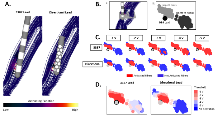
Figure 2: Comparison of central thalamic fiber bundle activation predictions with axisymmetric and directional DBS leads. (A) Visualization of both the Medtronic 3387 cylindrical DBS lead and the Sapiens directional DBS lead with activating function calculations on the target central thalamic fiber bundle for a single monopolar stimulation amplitude. (B)(i) A cross-sectional slice through the DBS lead and fiber bundles. (ii) A two-dimensional projection of the cross-sectional area with the identification of the DBS lead, target fibers, and fibers to avoid. (C) The spread of activation across both target fibers and fibers of avoidance as stimulation amplitude increases for both the axisymmetric and directional DBS lead. Activated fibers for a given stimulation amplitude are shown in red, while fibers not activated are shown in blue. (D) A compilation of all simulations shown in panel C, showing the predicted stimulation threshold amplitude across all regions of the fiber bundles. Please click here to view a larger version of this figure.

Discussion

This protocol has demonstrated techniques to reduce the time burden and computational cost of building patient specific models for DBS to a degree that allows near real-time feedback of simulation results. Rapid feedback enables the exploration of a large parameter space to better understand how parameter changes affect the model results. These parameters include lead location, choice of active contacts, and the amplitude, pulse width, and frequency of the stimulation waveform at those contacts. The key features of the proposed tool are: 1) A simple user interface to adjust the model parameters with near real-time visualization of how these parameters influence the simulation, and 2) Automation of model creation from a small set of inputs: the brain surface, brain tissue conductivity tensors, and a surface representation of the electrode geometry. This automation expedites the creation of patient-specific models for many individuals who have different brain geometries and tissue conductivities as well as evaluating the effects of inserting different electrode designs into existing models. The image pre-processing steps described in this protocol were not fully automated and can take up to a day of processing time. However, once completed the data generated from these steps are considered static, meaning this data is not modified during the simulations. The automation of model creation arises from the ability of the system to apply this data to the patient-specific FEM without manual effort. The SCIRun network to perform all of the model generation, simulation, visualization steps only needs to be built once. Therefore, only the image pre-processing steps need to be performed again to generate a patient-specific model for an incoming patient.

The performance gain in generating results from the modeling pipeline is due to the integration of mesh generation, bioelectric field calculations, and visualization of the solution into a single software environment. Existing modeling techniques such as adaptive mesh generation were used to create higher mesh density around the electrode and lower density farther from the electrode which reduces the time to build and solve the FEM. The software, SCIRun, also enables automation of the mesh generation and bioelectric field calculations. User-defined movement of the electrode using the interactive widgets triggers the construction of a new mesh with the updated electrode position. This includes modifying the boundary conditions and conductivity values for the new electrode position.

The electrode geometry is treated as a free-moving object inside of the brain volume before its position is integrated into the FEM. A key implication of this approach for mesh construction is that multiple electrodes can easily be inserted into the model. For example, a second copy of the electrode geometry can be placed several millimeters away and both will be included in the FEM. In recent research, two electrodes have been implanted in close proximity to treat multiple sclerosis tremor¹³ and have been used in non-human primate experiments to explore effective stimulation targets²¹. The benefit of using multiple electrodes is to provide better control of the electric field generated in the tissue over a larger area. Stimulating with active contacts on both electrodes can steer current towards the target region and away from regions that would lead to negative side effects. Finer control of stimulation over a larger area is also useful to explore different stimulation locations when the exact location of the intended target is unknown, as is the case with many of the emerging therapy applications of DBS. However, determining the parameters to achieve therapeutic stimulation is more challenging than a single electrode due to the increase in an already large parameter space.

We envision that this interactive modeling tool could provide benefit during pre-operative planning for DBS implantation. Feedback about the extent of stimulation in the brain tissue can allow surgeons to modify the electrode location in their surgical plan to provide therapeutic stimulation to the target region. While DBS therapy was the primary motivating factor for developing this tool, the techniques presented in this paper can be applied to any FEM bioelectric field model with different stimulation or recording paradigms. Stimulation therapies such as transcranial direct current stimulation for depression²² or the use of depth electrodes for the treatment of epilepsy²³ share the same challenges as DBS in determining the best location of stimulation to achieve therapeutic results. Electrocorticography, a recording technique with arrays of electrodes on the surface of the brain to identify seizure onset regions, has the challenge of determining where to place the electrodes to record from target regions in the brain²⁴. All of these applications are dependent on electrode position while dealing with the uncertainty of how current flows through the brain tissue. The techniques presented in this paper reduce the burden of generating and using computational models while providing meaningful feedback to researchers and clinicians using these devices who are not modeling experts.

Materials

List of materials used in this article

Name	Company	Catalog Number	Comments
FreeSurfer	Athinoula A. Martinos Center for Biomedical Imaging		https://surfer.nmr.mgh.harvard.edu/
3D Slicer	BWH, Harvard University		https://www.slicer.org/
SCIRun	University of Utah Center for Integrative Biomedical Computing		http://www.sci.utah.edu/cibc-software/scirun.html

References

- Benabid, A. L., et al. Chronic electrical stimulation of the ventralis intermedius nucleus of the thalamus as a treatment of movement disorders. Journal of Neurosurgery. 84 (2), 203-214 (1996).
- Limousin, P., et al. Effect of parkinsonian signs and symptoms of bilateral subthalamic nucleus stimulation. The Lancet. 345 (8942), 91-95 (1995).
- Schiff, N. D., et al. Behavioural improvements with thalamic stimulation after severe traumatic brain injury. Nature. 448 (7153), 600-603 (2007).
- Vandewalle, V., et al. Stereotactic treatment of Gilles de la Tourette syndrome by high frequency stimulation of thalamus. Lancet. 353 (9154), 724(1999).
- Mayberg, H. S., et al. Deep brain stimulation for treatment-resistant depression. Neuron. 45 (5), 651-660 (2005).
- Hashimoto, T., Elder, C. M., Okun, M. S., Patrick, S. K., Vitek, J. L. Stimulation of the subthalamic nucleus changes the firing pattern of pallidal neurons. Journal of Neuroscience. 23 (5), 1916-1923 (2003).
- York, M. K., Wilde, E. A., Simpson, R., Jankovic, J. Relationship between Neuropsychological Outcome and DBS Surgical Trajectory and Electrode Location. J. Neurol. Sci. 287 (1-2), 159-171 (2009).
- Machado, A., et al. Deep brain stimulation for Parkinson's disease: surgical technique and perioperative management. Movement Disorders. 21, S247-S258 (2006).
- Volkmann, J., Moro, E., Pahwa, R. Basic algorithms for the programming of deep brain stimulation in Parkinson's disease. Movement Disorders. 21 (S14), S284-S289 (2006).
- Contarino, M. F., et al. Directional steering: A novel approach to deep brain stimulation. Neurology. 83 (13), 1163-1169 (2014).
- Pollo, C., et al. Directional deep brain stimulation: An intraoperative double-blind pilot study. Brain. 137 (7), 2015-2026 (2014).
- Willsie, A. C., Dorval, A. D. Fabrication and initial testing of the µDBS: a novel deep brain stimulation electrode with thousands of individually controllable contacts. Biomedical Microdevices. 17 (56), 9961(2015).
- Oliveria, S. F., et al. Safety and efficacy of dual-lead thalamic deep brain stimulation for patients with treatment-refractory multiple sclerosis tremor: a single-centre, randomised, single-blind, pilot trial. The Lancet Neurology. 16 (9), 691-700 (2017).
- Butson, C. R., Cooper, S. E., Henderson, J. M., Wolgamuth, B., Mcintyre, C. C. Probabilistic Analysis of Activation Volumes Generated During Deep Brain Stimulation. Neuroimage. 54 (3), 2096-2104 (2011).
- Basser, P. J., Mattiello, J., LeBihan, D. MR diffusion tensor spectroscopy and imaging. Biophys. J. 66 (1), 259-267 (1994).
- Gullmar, D., Haueisen, J., Reichenbach, J. R. Influence of anisotropic electrical conductivity in white matter tissue on the EEG/MEG forward and inverse solution. A high-resolution whole head simulation study. NeuroImage. 51 (1), 145-163 (2010).
- Fischl, B. FreeSurfer. Neuroimage. 62 (2), 774-781 (2012).
- Fedorov, A., et al. 3D Slicer as an Image Computing Platform for the Quantitative Imaging Network. Magn. Reson. Imaging. 30 (9), 1323-1341 (2012).
- Jenkinson, M., Beckmann, C. F., Behrens, T. E., Woolrich, M. W., Smith, S. M. FSL. Neuroimage. 62 (2), 782-790 (2012).
- Medtronic DBS 3387/3389 Lead Kit Manual. , (2018).
- Baker, J. L., et al. Robust modulation of arousal regulation, performance and frontostriatal activity through central thalamic deep brain stimulation in healthy non-human primates. Journal of Neurophysiology. 116 (5), 2383-2404 (2016).
- Fregni, F., et al. Treatment of major depression with transcranial direct current stimulation. Bipolar Disorders. 8 (2), 203-204 (2006).
- Hodaie, M., Wennberg, R. A., Dostrovsky, J. O., Lozano, A. M. Chronic anterior thalamus stimulation for intractable epilepsy. Epilepsia. 43 (6), 603-608 (2002).
- Rosenow, F., Lüders, H. Presurgical evaluation of epilepsy. Brain. 124 (9), 1683-1700 (2001).
Reprints and Permissions