Isolation and Analysis of Microbial Communities in Soil, Rhizosphere, and Roots in Perennial Grass Experiments

Summary

Excavation of plant roots from the field as well as processing of samples into endosphere, rhizosphere, and soil are described in detail, including DNA extraction and data analysis methods. This paper is designed to enable other laboratories to use these techniques for the study of soil, endosphere, and rhizosphere microbiomes.

Abstract

Plant and soil microbiome studies are becoming increasingly important for understanding the roles microorganisms play in agricultural productivity. The purpose of this manuscript is to provide detail on how to rapidly sample soil, rhizosphere, and endosphere of replicated field trials and analyze changes that may occur in the microbial communities due to sample type, treatment, and plant genotype. The experiment used to demonstrate these methods consists of replicated field plots containing two, pure, warm-season grasses (Panicum virgatum and Andropogon gerardii) and a low-diversity grass mixture (A. gerardii, Sorghastrum nutans, and Bouteloua curtipendula). Briefly, plants are excavated, a variety of roots are cut and placed in phosphate buffer, and then shaken to collect the rhizosphere. Roots are brought to the laboratory on ice and surface sterilized with bleach and ethanol (EtOH). The rhizosphere is filtered and concentrated by centrifugation. Excavated soil from around the root ball is placed into plastic bags and brought to the lab where a small amount of soil is taken for DNA extractions. DNA is extracted from roots, soil, and rhizosphere and then amplified with primers for the V4 region of the 16S rRNA gene. Amplicons are sequenced, then analyzed with open access bioinformatics tools. These methods allow researchers to test how the microbial community diversity and composition varies due to sample type, treatment, and plant genotype. Using these methods along with statistical models, the representative results demonstrate there are significant differences in microbial communities of roots, rhizosphere, and soil. Methods presented here provide a complete set of steps for how to collect field samples, isolate, extract, quantify, amplify, and sequence DNA, and analyze microbial community diversity and composition in replicated field trials.

Introduction

Microbiome research has important implications for understanding and manipulating ecosystem processes such as nutrient cycling, organic matter turnover, and the development or inhibition of soil pathogens^1,2. This area of research also holds great potential for understanding the impacts of soil microbes on the productivity of natural plant communities and agroecosystems. While there are many studies that have focused on the soil microbiome in natural ecosystems, fewer have focused on plant rhizosphere and endosphere microbes in agroecosystems³. In Nebraska, agriculture dominates the landscape across large parts of the state, making the studies of these soils where agriculturally important crops are grown a vital topic for research. The aim of this methods paper is to provide researchers with a standard set of protocols to describe the microbes present in agroecosystems, to determine how plant roots modify the microbial communities in the rhizosphere and endosphere, and to eventually understand the functions these microbes play in soil health and plant productivity.

The method presented here differs slightly from methods used by others^4,5 in that this paper is aimed at learning which microbes are exclusively inside the root and how they differ from microbes immediately outside the root in the rhizosphere. The amplicon sequencing used in this study identifies the microbial taxa found in the DNA sample and allows investigators to determine how the communities change depending on sample type or treatment. One of the key differences between this protocol and a very similar protocol used by Lundberg et al.⁶ is that instead of sonication, this protocol uses surface sterilization with bleach and ethanol to remove the rhizosphere from the roots. Others have also used surface sterilization effectively^7,8,9,10. These methods are not more advantageous than other methods, but slightly different. These methods are particularly well suited for large field experiments because with enough people it is possible to process over 150 field plots per day, which adds up to approximately 450 samples when partitioned into endosphere, rhizosphere, and soil. This manuscript describes in detail the methods used to sample in the field, process the material in the lab, extract and sequence the DNA, and provides a brief overview of the steps to analyze the resulting sequencing data.

Protocol

1. Field Site Description

1. Describe experimental field sites during collection periods. Determine the location of field (latitude, longitude, and altitude) using a GPS.
2. Describe the sampling depth, sampling time, and soil texture.
3. Environmental factors play important roles in shaping microbial communities. Record climate information such as annual mean temperature, annual precipitation, prior years’ crop rotation, tillage practices, method of fertilization, and history of the field site. Automated weather stations or other devices are useful to record the daily rainfall and temperature over a growing season.

2. Collection and Processing of Soil, Rhizosphere, and Root Field Samples

1. Excavation of plants.
   1. Label a wash pan and bucket with a sticky note containing information about the plant material to be sampled. Include information such as plot number, plant genotype, and plant species. Carry the labeled bucket to the plot and leave the wash pan behind at the established workstation in the field.
   2. Pierce soil with a shovel to a depth of 30 cm to cut any of the lateral roots holding the plant in the soil. The approximate volume is 18 cm³. Randomly choose and collect two plants per plot from different areas within the plot.
   3. Excavate the plant roots by leveraging the shovel and place the root ball in the labeled bucket. Bring the labeled bucket with the excavated root ball back to the workstation in the field. Cut off and discard the aboveground plant biomass.
2. Removal of soil from roots and collection of bulk soil.
   1. Shake roots to manually remove soil or use a spade or a hand-held tiller to remove soil from the roots. Shaking the roots is sufficient to remove soil in very sandy soils. Wear gloves and place roots near the processing station.
   2. After shaking the roots, the bulk of the soil will be in the wash pan. Mix the soil in the wash pan and break up any soil clods with a hand-held tiller. Place a sample of soil that is free of debris into a labeled, 17.7 x 19.5 cm zipper storage bag and place in a cool place or on ice.
3. Collection of roots and rhizosphere.
   1. Using pruning scissors sterilized in 70% EtOH, excise a variety of roots, approximately 4 to 6 roots per plant and each root around 9 - 12 cm in length. Place the excised roots (cutting as needed to fit) in a labeled 50 mL tube containing 35 mL of autoclaved, phosphate buffer (6.33 g/L NaH₂PO₄, 8.5 g/L Na₂HPO₄ anhydrous, pH = 6.5, 200 µl/L surfactant).
      Note: The surfactant (see Table of Materials) was added after autoclaving the phosphate buffer. The volume of the root ball and root lengths vary depending on plant age and plant species.
   2. Shake tubes for 2 min to release the rhizosphere from the surface of the roots. With forceps sterilized in 70% EtOH, remove the roots from the tube, blot briefly on paper towels, and place in a new, labeled 50 mL tube. Place both the tube containing the rhizosphere and the one containing roots on ice.

3. Processing of Field Samples in the Laboratory

1. Surface sterilization of roots after field collection.
   Note: Perform surface sterilization as soon as possible after returning from the field. If it is not possible to surface sterilize the roots in the same day, store roots at 4 °C until processed.
   1. Add approximately 35 mL of 50% bleach + 0.01% Tween 20 to 50 mL root tubes collected in the field. Shake 50 mL tubes for 30 to 60 seconds. Pour off 50% bleach and add 35 mL of 70% EtOH. Shake for another 30 to 60 seconds.
   2. Pour off 70% EtOH and add 35 mL of sterile, ultrapure water. Shake for 1 minute. Repeat the water wash two more times.
      Note: To ensure our surface sterilization treatment is sufficient, we plated samples of water from the last rinse and observed no growth of bacteria (P. Wang, unpublished data, 2014). Other investigators have tested for root sterilization efficiency using similar methods^9,10.
   3. Blot roots dry on clean paper towels. Use a clean paper towel for each sample.
      Note: Paper towels can be sterilized before use. We do not sterilize our paper towels. However, we use 1 paper towel per sample and keep towels wrapped until used.
   4. Using sterile forceps and pruning scissors, cut the roots into approximately 5 mm pieces and place cut roots in a clean, labeled 15 mL conical tube. Store samples at -80 °C until further processed.
2. Processing rhizosphere samples.
   1. Shake 50 mL tubes containing rhizosphere samples from the field to resuspend the entire sample. Using a sterile, 100-µm-mesh cell strainer (see Table of Materials), filter the resuspended sample into a new 50 mL tube.
   2. Centrifuge the tubes at 3000 x g for 5 min at room temperature. Immediately pour off and discard the supernatant.
   3. Place rhizosphere pellets in the 50 mL tubes on ice. Add 1.5 mL of sterile phosphate buffer (without surfactant) to rhizosphere pellets and vortex to suspend.
   4. Pipet the suspended liquid into a clean, labeled, 2 mL microfuge tube. Spin tubes at 15,871 x g for 2 min at room temperature. Immediately pour off the supernatant and drain the tubes on clean paper towels.
   5. Store the pellets at -20 °C until further processed.
      Note: Steps 3.2.2 - 3.2.4 are done to reduce the sample tube size for storage. It is more space efficient to store the smaller 2 mL tubes compared to the 50 mL tubes.
3. Processing soil samples for DNA extraction and soil analysis.
   1. Using a sterile metal spatula, fill a clean, labeled 2 mL tube with approximately 3 g of soil for DNA extraction. Avoid any small root pieces and debris. Store this soil sample at -20 °C. Rinse metal spatula in 70% EtOH between each sample.
   2. In a clean wash pan, empty the bag of soil into stacked sieves (see Table of Materials), larger sieve on top of the smaller sieve, and manually sieve the soil through both sieves. Use a brush to carefully clean the sieves between samples.
   3. Set aside 100 to 125 g of sieved soil in a 17.7 x 19.5 cm zippered bag for future soil physicochemical and texture analysis. Place the bags of soil at 4 °C for short-term storage.
4. Processing soil samples for soil moisture.
   1. Tare a labeled brown paper bag on a scale. Measure 40 to 45 g of sieved soil into the brown paper bag. Record the weight of the brown paper bag and soil on a data sheet and place bags in a drying oven set to 55 - 60 °C.
   2. After 72 hours, remove the bags from the drying oven. Allow the soil bags to cool for at least 30 min and then weigh.
   3. To record the weight, tare the scale to zero and place the brown paper bags on the scale. Calculate the percentage of soil moisture for each sample using the formula:
      
      Note: The soil moisture method is from Kellogg Biological Station Long Term Ecological Research (KBS LTER). KBS LTER provides a wide range of established protocols for researchers on their website (https://Lter.kbs.msu.edu/).

4. Preparation of Processed Root Samples for DNA Extractions.

1. Grind frozen root material so that the sample is homogenous.
   1. Pour liquid nitrogen in a plastic beaker with clean spatulas and in a clean mortar and pestle to keep samples frozen throughout the grinding process.
   2. Place the frozen tissue in the mortar and grind with the pestle into a fine powder. Continually add liquid nitrogen throughout grinding to keep samples frozen.
   3. Use a spatula to place ground tissue in a clean, labeled 2 mL tube. Store at -80 °C.

5. Extraction of DNA from Soil and Rhizosphere Samples in 96-well Format

1. Loading soil samples into 96-well plates.
   1. Wipe down the work area with 70% EtOH and 1% bleach. Wear lab gloves during these steps. Remove the soil samples from -20 °C storage and allow to thaw in an ice bucket.
   2. Remove the sealing mat cover from a 96-well extraction plate that is provided with the DNA extraction kit. Place the sealing mat cover between 2 paper wipes to keep clean while not in use. To avoid contamination, use adhesive 8-well PCR strips to cover the 12 columns of the 96-well extraction plate.
   3. Tare a sterile weigh-funnel (size SM) on a scale and weigh out 200 to 250 mg of soil.
      Note: These sterile funnels are flattened on one side, so the funnel lays flat on a scale. The funnel is filled with soil and placed directly into a well. This technique avoids the loss of samples, minimizes spillage, and prevents cross-contamination.
   4. To uncover the first well of the extraction plate, carefully lift the adhesive strip up, place the neck of the filled weigh-funnel into the appropriate well, and gently guide the soil sample into the appropriate well. Replace the adhesive strip to cover the well.
   5. Repeat this process for every well of the plate, using a new, sterile funnel for each sample until the plate is filled. Leave one well empty as an extraction blank control.
      Note: One well is left blank on every extraction plate to serve as a negative (blank) control. This controls for contaminants that may be present in kit reagents¹¹.
   6. Replace the sealing mat cover on the extraction plate and store the plate at -20 °C until ready for DNA extraction.
2. Loading rhizosphere samples into 96-well plates.
   1. Remove the rhizosphere samples from -20 °C storage and allow to thaw in an ice bucket.
   2. Follow step 5.1.2 above to prepare the DNA extraction plate.
   3. Place a clean paper wipe on a scale, then tare a sterile metal spatula on the scale. Use the spatula to carefully scoop out some of the rhizosphere pellet from a sample tube. Return the spatula to the scale and weigh between 200 and 250 mg of the rhizosphere sample.
   4. Carefully lift the adhesive strip to uncover the first well of the extraction plate, angle the filled spatula into the well, and scrape off the rhizosphere material into the appropriate well with a sterile toothpick.
   5. Rinse the metal spatula in water, followed by 70% EtOH between samples. Repeat this process for every well of the plate until the plate is filled, leaving one well empty as an extraction blank control.
3. Extraction of DNA from rhizosphere and soil samples in 96-well format.
   1. Extract soil and rhizosphere DNA using a kit optimized for soil (see Table of Materials), following manufacturer’s protocol.
      Note: We use this specific kit to isolate soil and rhizosphere DNA because of the ability of the proprietary reagents to remove humic acid and other powerful PCR inhibitors found in soil.
4. DNA Quantification.
   1. Quantify 92 samples and 4 concentrations of standards using a kit (see Table of Materials; standards are included), according to manufacturer’s protocol.
   2. Quantify the remaining 4 samples that were removed from the plate to accommodate wells for the four standards using a kit (see Table of Materials), according to manufacturer’s protocol.

6. Extraction of DNA from Root Samples in 96-well Format.

1. Loading root samples into 96-well plates.
   1. Wipe down the work area with 70% EtOH and 1% bleach. Wear gloves during these steps.
   2. Keep ground root samples frozen at all times by placing samples in a bucket with dry ice.
   3. Fill a plastic beaker with liquid nitrogen and place antistatic microspatulas and sterile weigh-funnels (size XSM) in the plastic beaker to cool down.
   4. Remove the sealing mat cover from the 96-well extraction bead plate that is provided with kit and place it between 2 paper wipes to keep clean while not in use.
      Note: The newer version of this kit, released subsequent to the time we performed these DNA extractions, requires the user to supply the extraction bead plates. In the Table of Materials, we have listed the vendor catalog information needed to order these items.
   5. To avoid contamination, use adhesive 8-well PCR strips to cover the 12 columns of the 96-well extraction plate.
   6. Place the extraction bead plate on dry ice to keep samples in the wells frozen.
   7. Carefully lift the adhesive strip up to uncover the first well of the extraction plate, place the neck of the filled weigh-funnel into the appropriate well, and add 3 spatula scoops of ground root tissue. Replace the adhesive strip to cover the well.
      Note: The soil and rhizosphere are thawed on ice prior to weighing, whereas plant material is weighed out frozen. Frozen plant tissue, especially small amounts, is difficult to weigh on a scale without thawing. Weigh tests were done on ground root tissue to determine how many spatula scoops were sufficient. Note that the manufacturer of the kit does not require an exact amount of tissue but recommends around 50 mg. Different plant sample types will vary and the user will need to determine the appropriate amount.
   8. Repeat this process for every well of the plate until the plate is filled.
   9. Store plate at -20 °C until ready for DNA extraction.
2. DNA extraction of root tissue.
   1. Extract DNA using a kit optimized for plants (see Table of Materials) following the manufacturer's protocol.
      Note: We use this kit that is designed specifically for plant tissue to achieve maximum yields from the root samples. Unlike soil and rhizosphere, the humic acid and other contaminants are less of a problem for the root tissue.
3. Quantify the DNA as in step 5.4.

7. Amplification and Sequencing the Isolated DNA.

1. Amplify the V4 region of the 16S gene with a proof reading polymerase (see Table of Materials) as described in Gohl et al.¹² Barcode samples with different indexing primers and pool before sequencing. Sequence using the methods described by Gohl et al¹² using a two step PCR process with V4 primers (Supplemental File 1).
   Note: Some of the methods for these steps are described in detail elsewhere^12,13,14 and therefore will not be described here. For the root samples, PNA blockers were added to reduce the amount of plastid DNA amplified from the plant tissue, which has previously been fully described¹⁵. Two controls were used in sequencing, a negative control which included the extraction plate blank controls (see note after step 5.1.5), and a mock community of a known population of bacterial DNA (see Table of Materials) which served as a positive control.
   Note: In most cases, the MiSeq Reagent Kits v3 are used in the 2 X 300 base paired end mode. For the samples in this manuscript, the Illumina HiSeq 2500 was used in rapid mode with 250 Paired-end (2 x 250) mode. All the sample were sequenced in the same lane.
2. Process the sequencing data through a pipeline for microbial community analyses (USEARCH v9.2.64, QIIME v1.9.1 and RStudio v3.4.3 ¹⁶).
   1. Prepare the sequencing data using USEARCH¹⁷.
      Note: USEARCH is available online with full instructions (https://www.drive5.com/usearch/).
   2. Demultiplex the sequencing data using index reads or barcodes to assign Illumina reads to samples.
   3. Merge the paired-end reads to get consensus sequences. Use the command: usearch -fastq_mergepairs *R1*.fastq -relabel @ -fastq_maxdiffs 10 -fastq_minmergelen 230 -fastq_maxmergelen 320 -fastq_pctid 80 -fastqout merged.fq.
      Note: The parameters are set through referencing the USEARCH instruction manual.
   4. Remove the primers from the sequencing data to avoid substitutions in the primer sequences, which may be caused by the PCR reaction. Use the command: usearch -fastx_truncate merge.fq -stripleft 19 -stripright 20 -fastqout stripped.fq.
   5. Filter sequencing data to remove the low-quality reads and keep high quality operational taxonomic unit (OTU) sequences. Use the command: usearch -fastq_filter stripped.fq -fastq_maxee 1.0 -fastaout filtered.fa.
3. Generate OTUs in USEARCH.
   1. Perform the dereplication to identify the set of unique OTU sequences. Use the command: usearch -fastx_uniques filtered.fa -fastaout uniques.fa -sizeout -relabel Uniq.
   2. Cluster OTUs with 97 – 100% sequence similarity to designate the unique OTUs. Use the command: usearch -cluster_otus uniques.fa -minsize 2 -otus otus.fa -relabel Otu.
      Note: This step also incorporates the removal of singletons from the clustered OTUs and removal of chimeras from sequencing data.
   3. Create an OTU table in USEARCH. Use the command: usearch -usearch_global stripped.fq -db otus.fa -strand plus -id 0.97 -otutabout otutable.txt.
      Note: This command generates a table with the number of reads (counts) of all OTUs for each sample. The OTU table is used for downstream steps including differential abundance analyses and microbial diversity analyses. Example of OTU table is shown in supplemental figure 2.
   4. Conduct a rarefaction analysis in QIIME v1.9.1 ¹⁸.
      Note: The rarefaction curve is calculated using the OTU table to determine whether the depth of the sequencing properly samples the microbial community. Example of rarefaction curves are shown in Supplemental Figure 3.
   5. Conduct an alpha diversity analysis¹⁸. Use alpha_rarefaction.py in QIIME v1.9.1 to calculate the diversity of the microbial community within each sample.
      Note: This analysis calculates diversity indices such as Shannon¹⁹, Simpson²⁰, and Chao1²¹.
   6. Conduct a beta diversity analysis^18,22. Use the Python script: beta_diversity_through_plots.py in QIIME v1.9.1 Bray–Curtis dissimilarity matrix.
      Note: This analysis compares the microbial community composition between samples.
   7. Conduct statistical analyses between groups. Use the distance matrices calculated for PERMONOVA using the adonis and anova function in the vegan package²³ v2.4.5 in RStudio¹⁶. Conduct canonical analysis of principal coordinates (CAP) analysis using the capscale function in the vegan package. Visualize data using ggplot2 package²⁴ v2.2.1 in RStudio.

Results

The representative results presented in this manuscript come from a field site established in 2012 at the University of Nebraska-Lincoln Agriculture Research Division Farm near Mead, NE. Prior to the experiment, the site had been managed as a corn-soybean rotation. The study site was located on three different types of soils, but the data was analyzed as if all changes in measured soil properties were due to the treatments imposed.

The field site contained two, pure, stands of switchgrass (P. virgatum cv Liberty) and big bluestem (A. gerardii) as well as a low-diversity grass mixture containing big bluestem, indiangrass (S. nutans), and 'Butte' sideoats grama (B. curtipendula). The three warm-season grass plots were in a randomized complete block design that was replicated three times. Nested into the three different grass plots were two nitrogen (N) fertilization treatments, which were 56 (N1) and 112 (N2) kg N ha^-1 of applied urea. At the time of microbiome sampling at the end of the growing season, the soil contained 8.0 ± 1.1 (mean ± SD) ppm nitrate in the plots fertilized with 112 kg N ha^-1 and 6.8 ± 0.7 (mean + SD) ppm nitrate in the plots fertilized with 56 kg N ha^-1. The plots had been fertilized once a year. The warm-season grass plots were designated as the main plots (8000 m²) and N treatments were the split plots (4000 m²). Big bluestem was seeded as a 50:50 blend of 'Bonanza' and 'Goldmine' and Indiangrass was seeded as a 50:50 blend of 'Scout' and 'Warrior'. The plots were planted in 2012, and the first N application occurred in the spring of 2013.

The soil and root sampling was conducted on September 15, 2014. The work described below was conducted on a field that was set up as a split-plot randomized design with three replicates (Figure 1). The average sequencing depth of all the samples for endosphere were as follows: 4871 ± 5711 (mean ± SD), rhizosphere: 40726 ± 14684, soil: 38184 ± 9043. One of the largest sources of variation in these experiments, using the methods described, is the difference in microbial communities found between sample types (Figure 2). In this representative data set, the rhizosphere and soil appear to be more similar in composition to each other than the endosphere (Figure 2A). However, there were also highly significant (p = 0.001) differences in microbial community composition between rhizosphere and soil (Figure 2B). The total variation accounted for in these experiments analyzed by sample type was 26%.

Alpha diversity analysis showed that the microbial communities in the endosphere were lower in sample diversity as compared to soil and rhizosphere (Figure 3). The only significant differences in diversity between the grass species in any compartment were between the endosphere samples of big bluestem and switchgrass, with switchgrass having significantly higher microbial species diversity (Figure 3). The relative abundance analysis (Figure 4) highlights the dominance of Proteobacteria followed by Actinobacteria in all sample types. Soil and rhizosphere are also dominated by Acidobacteria and Chloroflexi whereas the endosphere had a larger relative abundance of Bacteriodetes.

In this experiment, plants were grown with two different amounts of N fertilizer and therefore we analyzed the data to determine whether there were treatment effects. Treatment effects accounted for 12% of the total variation but were not significantly different although in the ordination the two treatments look different (Figure 5). This highlights the importance of statistical analyses for these datasets rather than visual inspection or qualitative judgments.

Plant-influenced differences in the microbiome of plant tissues and soil were visualized using a constrained method of ordination. Statistical differences were determined using a PERMANOVA analysis to test whether specific variables, such as species, result in significantly different microbial community composition between samples. When all the sample types were analyzed together, a highly significant difference was found in microbial community composition due to plant species (Figure 6). In this experiment, the amount of variation accounted for by plant species was 6.7%. Finally, each sample type was analyzed individually to determine which of the sample types might be driving the significant plant species effect. Only in the endosphere was there a highly significant difference (p = 0.001) between the microbial community compositions of the different plant species (Figure 7). In the other sample types, the species effect was not significant when analyzed individually. In the endosphere, the percent variation due to species was 27%, whereas it was lower in rhizosphere (18%) and soil (15%). This further highlights the importance of analyzing each tissue type individually.

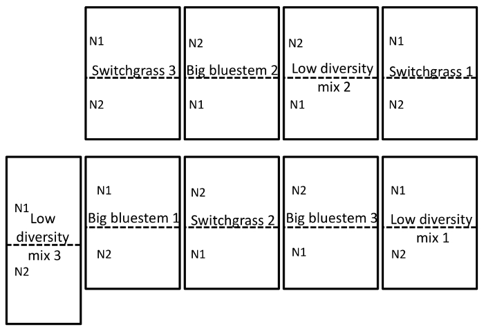
Figure 1: Example of the experimental field design. Experimental field design illustrating a randomized complete block design in triplicate of the field site located at the University of Nebraska-Lincoln Eastern Nebraska Research and Extension Center near Mead, NE. For full site description see the Results section. N1 is the low (56 kg N ha^-1 urea) and N2 (112 kg N ha^-1 urea) is the higher nitrogen rate that was applied. Please click here to view a larger version of this figure.

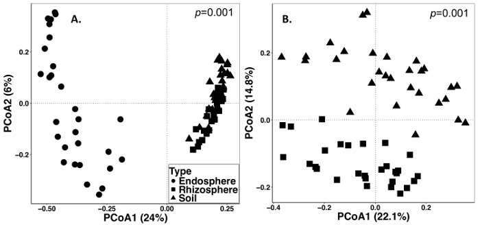
Figure 2: Beta diversity analysis comparing the microbial composition in the different sample types including endosphere, rhizosphere, and soil from the perennial grass sampling in 2014. The analysis was carried out using a Python script in QIIME1.9.1 to produce the Bray-Curtis dissimilarity matrix. Principal coordinates analysis (PCoA) based on the Bray-Curtis dissimilarity matrix was visualized in RStudio. PCoA1 and PCoA2 indicate the first and second largest variance explained by the PCoA analysis. PERMANOVA statistical analysis was performed to determine the significance between sample types, and the p value is shown on the top right corner. Each symbol in the figures represent the entire microbial community for each sample. (A) Endosphere, rhizosphere and soil sample types were analyzed together. All 87 samples were rarefied to 486 sequences per sample. (B) Rhizosphere and soil samples were analyzed together. All 59 samples were rarefied with 8231 sequences. Please click here to view a larger version of this figure.

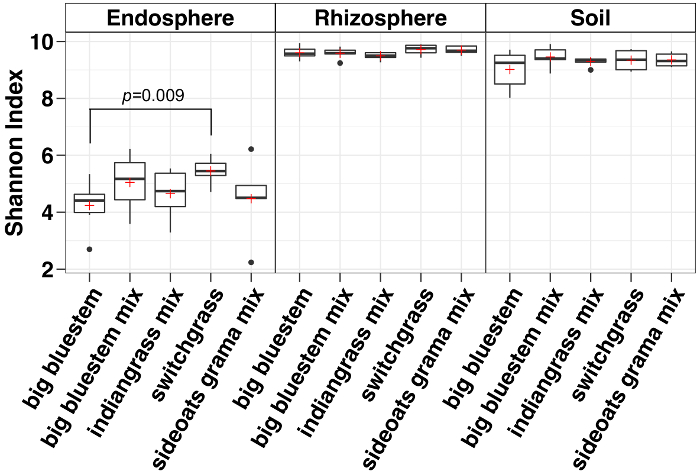
Figure 3: Alpha diversity analysis using Shannon index for each species in the endosphere, rhizosphere and soil. The analysis was carried out using a Python script in the QIIME1.9.1. Rarefaction was done for the endosphere, rhizosphere, and soil sample types respectively with 486, 17154 and 8231 sequences per sample. Boxes indicate the 25th and 75th percentiles (first and third quartiles). The horizontal line within the box denotes the median and the red plus shows the mean. Whiskers show the range of the data excluding outliers (which are shown as black dots) that fell more than 1.5 times the interquartile range (n = 6 for each sample except for sideoats grama mix where n = 5). The Shannon index of all five species in the endosphere were lower than both rhizosphere and soil. Non-parametric Wilcoxon rank sum test was used to determine the significance between the species and only significant differences between species were shown on top of the boxes. Please click here to view a larger version of this figure.

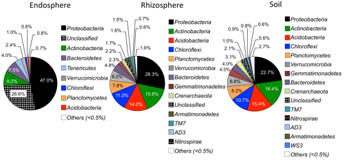
Figure 4: Relative abundance on the phylum level in the endosphere, rhizosphere, and soil. Samples were analyzed to compare the abundance of microbial phyla among different samples types (n = 29 for each sample type). The analysis was carried out using a Python script in QIIME1.9.1 from the OTU table. The different colors inside the pie chart denote the phyla. The percentage indicates the relative abundance of each phylum in each sample type. The phylum information was annotated using the Ribosomal Database Project classifier (RDP)²⁵. Please click here to view a larger version of this figure.

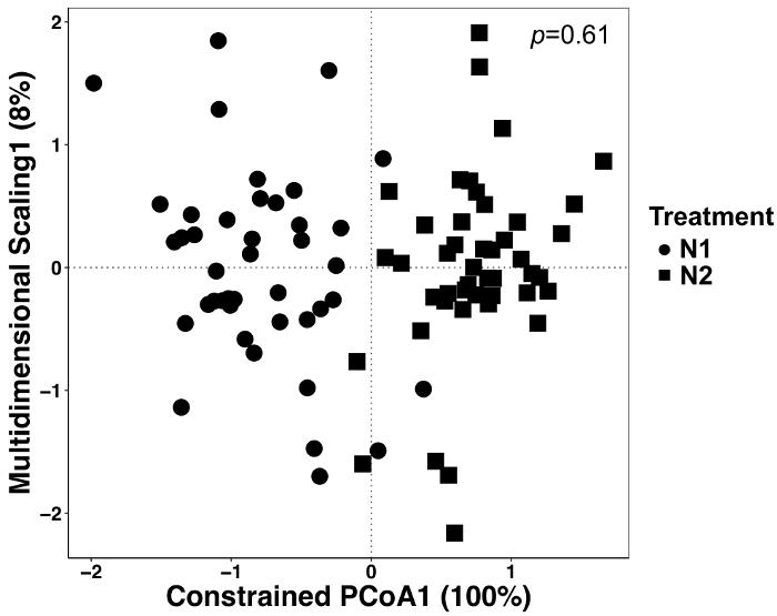
Figure 5: Analysis using treatment as constraining factor between all sample types. Canonical analysis of principal coordinates (CAP) analysis was performed to determine whether there were differences in microbial community composition between treatments. For each N treatment, n = 42 for N1 (56 kg N ha^-1) and n = 45 for N2 (112 kg N ha^-1). The Bray-Curtis dissimilarity matrix was generated using a python script in the QIIME1.9.1. CAP analysis based on the Bray-Curtis dissimilarity matrix was done by constraining the treatment as the factor in RStudio. PERMANOVA analysis was performed to determine whether treatment differences were significant, and the p value is shown on the top right corner. Please click here to view a larger version of this figure.

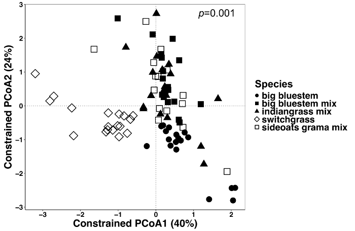
Figure 6: Analysis using plant species as constraining factor between all sample types. Analysis was conducted to determine whether there were differences in the microbial community composition between plant species in all sample types. Principal coordinates ordination and CAP analysis of all sample types (endosphere, rhizosphere, and soil) were done using a Bray-Curtis dissimilarity matrix. The Bray-Curtis dissimilarity matrix was generated using the Python script in QIIME1.9.1. CAP analysis based on the Bray-Curtis dissimilarity matrix was done by constraining the plant species as the factor in RStudio. PERMANOVA statistical analysis was performed to determine the significance between plant species, and the P value is shown on the top right corner. Each symbol in the figures represents the entire microbial community for that sample. n = 18 for each species in all sample types except n = 15 for the sideoats grama mix. Please click here to view a larger version of this figure.

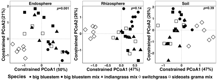
Figure 7: Example of CAP analysis using species as constraining factor for each sample type individually. Principal coordinate ordination and CAP analysis of each sample type (endosphere, rhizosphere, and soil) using Bray-Curtis dissimilarity matrix. Each sample type was rarefied to 486, 17154, and 8231 reads per sample respectively in endosphere, rhizosphere and soil. Species was used as the factor to constrain the ordination. PERMANOVA statistical analysis was performed to determine the significance between plant species in each sample type, and the p value is shown on the top right corner. Each symbol in the figure represents the entire microbial community for each sample. Sample size is n = 29 for each sample type, n = 6 for each plant species in each sample type except for the sideoats grama mix (n = 5). Please click here to view a larger version of this figure.

Discussion

The methods described in this manuscript should enable scientists to easily enter the field of soil and plant metagenomics. Over the years, we have refined our methods since conducting the experiment described in this manuscript. One change is that we now pre-label tubes before going out to the field to sample. Our lab uses a barcoding system and a label printer. The label printer not only saves time when labeling tubes, but also makes everything easier to track and to correctly identify samples without the vagaries of human hand writing. Another critical point is that we try to process the material after bringing it back from the field as soon as possible. We aim to freeze the soil used for DNA analysis, sterilize and freeze the roots, and filter and freeze the rhizosphere within 12 to 36 hours after returning from the field. The DNA extraction procedures are lengthy with many steps, particularly for soil and rhizosphere, so we purchased a robot (Kingfisher Flex, ThermoFisher) that minimizes the hands on time for the DNA extraction protocols, reduces human error that may be introduced, and improves the consistency in the way different batches of soil, roots, or rhizosphere are processed. When working with plant material it is important to decide on the root type to be studied or to take a variety of root types to get a "representative sample". Maintaining roots and leaves in a frozen state when conducting the DNA extractions is important, as is ensuring there is no cross-contamination between samples when filling 96-well DNA extraction plates. Another important factor to consider is the number of replicates to be used when designing field experiments and using a complete randomized design where possible²⁶. Due to high field variability it may be necessary to have a large number of replicates to detect small differences. Finally, from our experience it is essential to make sure soils are not too wet when excavating the roots. If the soils are saturated with water it is not only messy to work with, but it is also very difficult to define the rhizosphere and to remove the soil from the roots.

One modification that was made early on during the development of these methods was instead of shaking the tubes by hand to release the rhizosphere we upgraded to vortexers powered by a gas generator to make the work easier in the field and more standardized in terms of the time and manner that each tube was agitated. One limitation of the amplicon sequencing approach is that the taxonomic resolution of the results is often limited and many OTUs are unknown or only known at the family or genus level. This field of research is rapidly evolving so it is important to be aware of new and developing approaches, particularly for data analysis that may enhance the resolution of the results.

These protocols are only for studying bacteria and archaea, not fungi. The use of different primers for amplification will allow for the study of fungal communities using the same DNA samples^27,28. These methods do not require the purchase of large amounts of equipment because the methods can be simplified. The methods we describe here are mainly for determining "who is there", but the field is quickly evolving into asking important questions about function, which may be addressed by using shotgun sequencing methods, isolation and testing the functionality of microbes, or sequencing whole microbial genomes.

The representative results highlight the differences in microbial communities that may be identified using the methods described. Using a beta-diversity approach to the data analysis²², compositional differences were shown between sample types. These difference have been clearly observed in most other studies where endosphere, rhizosphere, and soil contain unique microbial communities³. The Shannon diversity index was calculated to determine the abundance and evenness of the microbial species present within each plant species in the endosphere, rhizosphere, and soil. As shown in this study and in many others, alpha diversity is highest in the soil, decreasing slightly in the rhizosphere and then decreasing significantly in the endosphere^3,5,29. These results indicate that the methods described here are suitable for identifying compositional changes in the endosphere, rhizosphere, and soil.

The dominance of the Proteobacteria is a common finding in studies on endosphere and soil^30,31,32. Endosphere generally has a lower diversity of microbial species with a higher relative abundance of the Proteobacteria. This again highlights that the results here are representative of other findings in the literature. The treatment effects in this study were not significantly different and two major reasons for that may be that the differences imposed by the treatments were not large enough to generate sufficient variation to detect and that this sampling was done at the end of the growing season, when the fields may have had sufficient time to draw down the nitrogen to similar levels, which is what was measured at the end of the season. In another study using similar fertilization rates over a longer period of time, only relatively small changes in the composition of the microbiome were measured³³. Other studies have shown changes in both fungal and bacterial communities due to nitrogen fertilizer^34,35.

Plant species are known to play roles in determining their microbiomes^3,32,36 and even small differences in microbial community variation have been demonstrated between different plant genotypes within a single species³⁷. In this study, a significant difference in microbial community composition was found between plant species. In all the sample types it appeared that switchgrass had the most distinct microbial composition, but differences between species were only statistically significant in the endosphere. Rhizosphere community composition may have become significant if more replicates were available for analysis.

The combined field, lab, and analytical protocols described here provide a powerful method for studying how different factors influence the composition of microbial communities in soils, rhizosphere, and the endosphere of roots³⁶. There is a great deal of work to be done in the area of studying microbiomes, particularly in agricultural fields. Important questions about how yields are altered by the soil microbiome have yet to be fully elucidated. Even the most basic questions regarding how crop rotations influence the soil microbiome, how timing alters the microbiome, how abiotic stress alters the microbiome, how soil type interacts with these factors to alter the microbiome, and whether there are universal microbes in certain crops or regions of the USA are all open questions. These methods will also be useful for epidemiological studies to identify the presence and persistence of pathogenic and beneficial bacteria. Another future horizon for these methods will be to start integrating the DNA methods described here with plant and microbe RNA and metabolite data. Additional improvement and testing of more variables will be important for further optimization of these protocols.

Materials

List of materials used in this article

Name	Company	Catalog Number	Comments
Dneasy PowerSoil HTP 96 Kit	Qiagen/MoBio	12955-4	Extraction kit for soil and rhizosphere
Dneasy PowerPlant HTP 96 Kit	Qiagen/MoBio	13496-4	Extraction kit for roots
D-Handle Digging shovel, 101 cm L	Fiskars	9669
Rapid Tiller, 40 cm L	Truper	34316
Ziploc Bags, 17.7 cm x 19.5 cm	Ziploc	NA
Cooler	Any	NA
Wash pan	Any	NA
Plastic bucket	Any	NA
Gloves (work and lab)	Any	NA
20 cm diameter Soil sieve #8, 2360 μm mesh size	Dual Manufacturing Co., Chicago IL	US8-8FS
20 cm diameter Soil Sieve #4, 4750 μm mesh size	Dual Manufacturing Co., Chicago IL	US8-4FS
portable generator	Honda brand works well	NA
Sterile cell strainers 100 μm mesh size	Fisher Scientific	22-363-549
NaH2PO4·H2O	VWR	0823
Na2HPO4	VWR	0404
Silwet L-77	Lehman Seeds	VIS-30	Surfactant
Autoclaves	Any	NA
Drying Oven	Any	NA
Scale	Any	Any
Bleach	CLOROX - household strength	NA
Tween 20	Any	NA
Liquid Nitrogen	Any	NA
Dry Ice pellets	Any	NA
Ethanol	Any	NA
11 cm precision fine point tweezers	Fisher	17456209
18 cm Straight point specimen forceps	VWR	82027-436
13.5 cm Pruning Scissors	Fiskars	9921
2 mL tube	Any	NA
15 mL PP conical tube	MIDSCI	C15B
50 mL PP conical tube	MIDSCI	C50B
Ultrapure water	Millipore-sigma	Milli-Q Integral, Q-POD
Qubit 2.0 fluorometer	Invitrogen	Q32866
Qubit dsDNA HS Assay Kit	Invitrogen	Q32854	For DNA quantification of removed samples
QuantiFluor dsDNA System	Promega	E2670	For DNA quantification
96-Well Black with Clear Flat Bottom Plates	Corning	3631
pPNA PCR Blocker	PNA Bio	PP01-50
mPNA PCR Blocker	PNA Bio	MP01-50
Genomic DNA from Microbial Mock Community B (Even Low Concentration) v5.1L, for 16s rRNA Gene sequencing	BEI Resources	HM782D
Adhesive 8 well-strips for plates	VWR	89134-434
Stainless steel beads, 3.2 mm dia	Next Advance	SSB32
1 ml Assay block (DNA extraction plate for the Qiagen/MoBio Dneasy PowerPlant HTP Kit)	CoStar	3959
antistatic PP weighing funnel, size small for soil/rhizosphere	TWD Tradewinds, INC	ASWF1SPK
antistatic PP weighing funnel, size x-small for root/leaf	TWD Tradewinds, INC	ASWFXSCS
Genie 2 Digital Vortex	Scientific Industries	SI-0236
Vortex adapter for 50 mL tubes	Scientific Industries	SI-H506
Mortar (100 mL) and pestle	Any	NA
Metal micro-spatula	VWR	80071-672
Disposable antistatic microspatulas	VWR	231-0106
Brown Paper bag 2# (10.95 cm x 6.19 cm x 20 cm)	Duro	18402
5424 Centrifuge for 2 mL tube	Eppendorf	22620461
Centrifuge for 96-well plate	Sigma4-16S	81510
Centrifuge rotor for 50 mL tubes	Sigma4-16S	12269 - Biosafe
KAPA HiFi DNA polymerase	Kapa Biosystems

References

- Philippot, L., Raaijmakers, J. M., Lemanceau, P., vander Putten, W. H. Going back to the roots: the microbial ecology of the rhizosphere. Nature Reviews Microbiology. 11, 789-799 (2013).
- Fierer, N. Embracing the unknown: disentangling the complexities of the soil microbiome. Nature Review Microbiology. 15 (10), 579-590 (2017).
- Wang, P., et al. Shifts in microbial communities in soil, rhizosphere and roots of two major crop systems under elevated CO2 and O3. Scientific Reports. 7 (1), 15019(2017).
- White, L. J., Jothibasu, K., Reese, R. N., Brözel, V. S., Subramanian, S. Spatio Temporal influence of isoflavonoids on bacterial diversity in the soybean Rhizosphere. Molecular Plant-Microbe Interactions. 28 (1), 22-29 (2015).
- Edwards, J., et al. Structure, variation, and assembly of the root-associated microbiomes of rice. Proceedings of the National Academy of Science of the United States of America. 112 (8), E911-E920 (2015).
- Lundberg, D. S., et al. Defining the core Arabidopsis thaliana root microbiome. Nature. 488, 86-90 (2012).
- Bougoure, D. S., Cairney, J. W. Assemblages of ericoid mycorrhizal and other root-associated fungi from Epacris pulchella (Ericaceae) as determined by culturing and direct DNA extraction from roots. Environmental Microbiology. 7 (6), 819-827 (2005).
- Doty, S. L., et al. Diazotrophic endophytes of native black cottonwood and willow. Symbiosis. 47 (1), 23-33 (2009).
- Gottel, N. R., et al. Distinct microbial communities within the endosphere and rhizosphere of populus deltoides roots across contrasting soil types. Applied and Environmental Microbiology. 77 (17), 5934-5944 (2011).
- Xin, G., Glawe, D., Doty, S. L. Characterization of three endophytic, indole-3-acetic acid-producing yeasts occurring in Populus trees. Mycological Research. 113, 973-980 (2009).
- Salter, S. J., et al. Reagent and laboratory contamination can critically impact sequence-based microbiome analyses. BMC Biolology. 12, 87(2014).
- Gohl, D. M., et al. Systematic improvement of amplicon marker gene methods for increased accuracy in microbiome studies. Nature Biotechnology. 34 (9), 942-949 (2016).
- Kozich, J. J., Westcott, S. L., Baxter, N. T., Highlander, S. K., Schloss, P. D. Development of a dual-index sequencing strategy and curation pipeline for analyzing amplicon sequence data on the MiSeq Illumina sequencing platform. Applied Environmental Microbiology. 79 (17), 5112-5120 (2013).
- Caporaso, J. G., et al. Ultra-high-throughput microbial community analysis on the Illumina HiSeq and MiSeq platforms. ISME Journal. 6 (8), 1621-1624 (2012).
- Lundberg, D. S., Yourstone, S., Mieczkowski, P., Jones, C. D., Dangl, J. L. Practical innovations for high-throughput amplicon sequencing. Nature Methods. 10 (10), 999-1002 (2013).
- RStudio, T. RStudio: Integrated Development for R. RStudio, Inc. , Available from: http://www.rstudio.com/ (2015).
- Edgar, R. C. UPARSE: highly accurate OTU sequences from microbial amplicon reads. Nature Methods. 10 (10), 996-998 (2013).
- Caporaso, J. G., et al. QIIME allows analysis of high-throughput community sequencing data. Nature Methods. 7 (5), 335-336 (2010).
- Shannon, C. A mathematical theory of communication. Bell System Technical Journal. 27, 379-423 (1948).
- Simpson, E. H. Measurement of diversity. Nature. 163, 688(1949).
- Chao, A. Non-parametric estimation of the number of classes in a population. Scandanavian Journal of Statistics. 11, 265-270 (1984).
- Legendre, P. Studying beta diversity: Ecological variation partitioning by multiple regression and canonical analysis. Journal of Plant Ecology. 1 (1), 3-8 (2008).
- Oksanen, J., et al. The vegan package. Community Ecology Package. 10, 631-637 (2007).
- Wickham, H. ggplot2: Elegant graphics for data analysis. Ggplot2: Elegant Graphics for Data Analysis. , Springer Nature. Switzerland. 1-212 (2009).
- Cole, J. R., et al. The Ribosomal Database Project (RDP-II): sequences and tools for high-throughput rRNA analysis. Nucleic Acids Research. 33, D294-D296 (2006).
- Wagner, M. R., et al. Host genotype and age shape the leaf and root microbiomes of a wild perennial plant. Nature Communications. 7, 12151(2016).
- O'Brien, H. E., Parrent, J. L., Jackson, J. A., Moncalvo, J. M., Vilgalys, R. Fungal community analysis by large-scale sequencing of environmental samples. Applied and Environmental Microbiology. 71 (9), 5544-5550 (2005).
- Taylor, D. L., et al. A first comprehensive census of fungi in soil reveals both hyperdiversity and fine-scale niche partitioning. Ecological Monographs. 84 (1), 3-20 (2014).
- Lebeis, S. L., et al. Salicylic acid modulates colonization of the root microbiome by specific bacterial taxa. Science. 349 (6250), 860-864 (2015).
- Ofek-Lalzar, M., et al. Niche and host-associated functional signatures of the root surface microbiome. Nature Commununications. 5, 4950(2014).
- Niu, B., Paulson, J. N., Zheng, X., Kolter, R. Simplified and representative bacterial community of maize roots. Proceedings of the National Academy of Science of the United States of America. 114 (12), E2450-E2459 (2017).
- Fitzpatrick, C. R., et al. Assembly and ecological function of the root microbiome across angiosperm plant species. Proceedings of the National Academy of Science of the United States of America. 115 (6), E1157-E1165 (2018).
- Ramirez, K. S., Lauber, C. L., Knight, R., Bradford, M. A., Fierer, N. Consistent effects of nitrogen fertilization on soil bacterial communities in contrasting systems. Ecology. 91 (12), 3463-3470 (2010).
- Paungfoo-Lonhienne, C., et al. Turning the table: Plants consume microbes as a source of nutrients. PLoS One. 5 (7), e11915(2010).
- Yeoh, Y. K., et al. The core root microbiome of sugarcanes cultivated under varying nitrogen fertilizer application. Environmental Microbiology. 18 (5), 1338-1351 (2016).
- Bulgarelli, D., Schlaeppi, K., Spaepen, S., Ver Loren van Themaat, E., Schulze-Lefert, P. Structure and functions of the bacterial microbiota of plants. Annual Review of Plant Biology. 64, 807-838 (2013).
- Peiffer, J. A., et al. Diversity and heritability of the maize rhizosphere microbiome under field conditions. Proceedings of the National Academy of Science of the United States of America. 110 (16), 6548-6553 (2013).
Reprints and Permissions