Nuclei Isolation from Fresh Frozen Brain Tumors for Single-Nucleus RNA-seq and ATAC-seq

Summary

Intra-tumoral heterogeneity is an inherent feature of tumors, including gliomas. We developed a simple and efficient protocol that utilizes a combination of buffers and gradient centrifugation to isolate single nuclei from fresh frozen glioma tissues for single nucleus RNA and ATAC sequencing studies.

Abstract

Adult diffuse gliomas exhibit inter- and intra-tumor heterogeneity. Until recently, the majority of large-scale molecular profiling efforts have focused on bulk approaches that led to the molecular classification of brain tumors. Over the last five years, single cell sequencing approaches have highlighted several important features of gliomas. The majority of these studies have utilized fresh brain tumor specimens to isolate single cells using flow cytometry or antibody-based separation methods. Moving forward, the use of fresh-frozen tissue samples from biobanks will provide greater flexibility to single cell applications. Furthermore, as the single-cell field advances, the next challenge will be to generate multi-omics data from either a single cell or the same sample preparation to better unravel tumor complexity. Therefore, simple and flexible protocols that allow data generation for various methods such as single-nucleus RNA sequencing (snRNA-seq) and single nucleus Assay for Transposase-Accessible Chromatin with high-throughput sequencing (snATAC-seq) will be important for the field.

Recent advances in the single cell field coupled with accessible microfluidic instruments such as the 10x genomics platform have facilitated single cell applications in research laboratories. To study brain tumor heterogeneity, we developed an enhanced protocol for the isolation of single nuclei from fresh frozen gliomas. This protocol merges existing single cell protocols and combines a homogenization step followed by filtration and buffer mediated gradient centrifugation. The resulting samples are pure single nuclei suspensions that can be used to generate single nucleus gene expression and chromatin accessibility data from the same nuclei preparation.

Introduction

Diffuse lower grade gliomas (LGG), the most common primary brain tumor in adults, are infiltrative neoplasms that often arise in the cerebral hemisphere. LGGs exhibit both inter- and intra-tumor heterogeneity, which is not only driven by the tumor population but also by the non-malignant cells intricately involved in tumor development and progression^1,2,3,4,5.

Over the last decade, there has been an avalanche of genomic data gathered in the field of gliomas. These data mainly come from bulk tumor sequencing studies and have contributed immensely to the molecular characterization, and the current classification of brain tumors^{5,6,7,8,9,10,11}. However, even though these studies revealed the broad molecular landscape associated with gliomas, there is still a disappointing lack of progress regarding therapeutic intervention. One of the obstacles to treatment resistance in brain tumors is intra-tumor heterogeneity. To address this issue, various studies have been focusing on the genomic, transcriptomic, proteomic, and epigenetic heterogeneity present within a tumor at a single cell level^{12,13,14,15,16,17}.

Although there have been remarkable technological advancements in the single cell field over the last couple of years, one of the major limiting factors is the availability of fresh specimens needed to isolate the cells and perform these experiments. To overcome this limitation, there have been several successful attempts at performing assays, such as snRNA-seq and snATAC-seq from frozen tissues, using nuclei rather than cells^18,19. The majority of these methods rely on either fluorescence-activated cell sorting (FACS) or filtration strategies. Both single cell and single nuclei approaches have their strengths and drawbacks. Single cell approaches maintain mitochondrial transcripts, which although may be informative, can also reduce transcriptome coverage due to their high abundance. Single nuclei isolation approaches eliminate a high percentage of the mitochondrial fraction, thereby allowing a more in-depth coverage of the nuclear transcripts²⁰.

There are various commercially available platforms that have been used over the recent years to assay single cell genomics data, including RNA-seq and ATAC-seq. One of the most prominent platforms is the 10x Genomics Chromium platform for single cell gene expression and single cell ATAC profiling. As the platform works with the help of microfluidic chambers, any debris or aggregates can clog the system leading to loss of data, reagents, and valuable clinical samples. Therefore, the success of single cell studies depends largely on the accurate isolation of single cells/nuclei.

The protocol that we will demonstrate herein is a slightly modified combination of the DroNc-seq and Omni-ATAC-seq protocols, and utilizes a similar approach to recent studies that utilize snRNA-seq to understand neurological disorders and neuronal cell types in the human brain^{18,19,21,22,23,24}. The protocol uses a combination of enzymatic/mechanical dissociation of frozen samples followed by filtration and gradient centrifugation and allows for fast and accurate isolation of single nuclei from fresh frozen glioma tissues. We have successfully used this protocol to generate snRNA-seq and snATAC-seq data from the same nuclei preparation from brain tumor specimens.

Protocol

Fresh frozen glioma samples were obtained from the National Center for Tumor diseases (NCT)-tissue bank in Heidelberg, Germany. The use of patient material was approved by the Institutional Review Board at the Medical Faculty of Heidelberg, and informed consent was obtained from all patients included in the study.

1. Experimental preparation

1. Perform all steps on ice or at 4 °C.
2. Pre-chill tubes, dishes, razor blades, Douncers and pestles to 4 °C.
3. Prepare all buffers in advance. These buffers are stable at room temperature. Sterile filtration is recommended, especially for sucrose. The stock preparations are modified from Corces et al.¹⁹. See Tables 1-7.
4. Remove samples from liquid nitrogen or -80 °C freezer storage and keep on dry ice until Step 2.1.

2. Tissue dissection and dissociation

1. Transfer fresh frozen tissue sample (10-60 mg) to a pre-chilled Petri dish. Mince/chop fresh frozen tissue with a razor blade to small pieces on ice.
2. Add 500 µL of chilled nuclei lysis buffer to a pre-chilled 1.5 mL tube. Place the tissue pieces in the 1.5 mL tube containing the nuclei lysis buffer, and transfer to a Douncer (Table of Materials).
   NOTE: There are two Dounce homogenizer pestles: “loose” or “A” pestle for initial sample reduction and “tight” or “B” pestle for complete sample homogenization.
3. Dounce the tissue pieces with the “loose” pestle for about 20 strokes, until friction is reduced. If debris is present, the sample may be pre-cleared by filtration with a 100 mm strainer.
4. Dounce with the “tight” pestle for 20 strokes to achieve complete tissue homogenization.
5. Transfer the homogenate (about 500 µL) into a pre-chilled 2 mL tube. Add 1 mL of chilled lysis buffer. Mix gently and incubate on ice for 5 min. Gently mix with a wide-bore pipette tip and repeat 1-2 times during the incubation.
6. Filter the entire homogenate using a 30 µm strainer mesh, collect into a 15 mL Falcon tube and transfer back into a new pre-chilled 2 mL tube. A single strainer is typically sufficient for the entire homogenate.
7. Check under a light microscope to verify the removal of large debris and the intactness of the nuclear membrane. Nuclei need to be round and the nuclear membrane should not be distorted. If debris is present, nuclei can be re-filtered.
8. Centrifuge the nuclei at 500 x g for 5 min at 4 °C on a bench top centrifuge. Remove the supernatant, leaving behind ~50 µL with pellet containing the nuclei. Gently resuspend the pellet in another 1 mL of nuclei lysis buffer and incubate for 5 min on ice.
9. Centrifuge the nuclei at 500 x g for 5 min at 4°C. Remove the supernatant without disturbing pellet, add 500 mL of 1x homogenization buffer (HB) (Table 4) and incubate for 5 min without resuspending. Then, resuspend the nuclei in another 1.0 mL of 1x HB.
10. Centrifuge the nuclei at 500 x g for 5 min at 4 °C. Remove the supernatant and gently resuspend the nuclei in 200 µL of 1x HB into a new 2.0 mL tube.

3. Gradient centrifugation

1. Add 200 µL of 50% iodixanol solution (Table 5) to give a final concentration of 25% iodixanol. Mix well 10 times with pipette set on 300 mL.
2. Add 300 µL of 29% iodixanol solution (Table 6) under the 25% mixture. Use a P1000 fine tip to avoid mixture of the layers.
3. Add 300 µl of 35% Iodixanol solution (Table 7) under the 29% mixture. Use a P1000 fine tip to avoid mixture of the layers.
   Caution: This step requires gradual removal of the pipette tip during pipetting to avoid excessive volume displacement.
4. Place the samples in a swinging bucket centrifuge, spin for 20 min at 3,500 x g at 4°C with the brake off.
5. Gently remove the samples without shaking and observe under light. A clear white band of 95% pure nuclei should be visible between the second and third layer (Figure 1).

4. Isolation of nuclei

1. Aspirate the top layers until the white nuclei band at the interphase of 29%-35%.
2. Collect the nuclei band in a 200 mL volume, transfer to a fresh tube and filter with a 20 µm filter (Table of Materials).
   NOTE: The nuclei do not need to be resuspended prior to filtration.
3. Check under a light microscope to verify the removal of large debris and the intactness of the nuclear membrane. Nuclei need to be round and the nuclear membrane should not be distorted.
4. Count nuclei using Trypan blue staining on a hemocytometer and aliquot nuclei for snRNA-seq/snATAC-seq.

5. Single nuclei RNA and ATAC seq

1. Immediately process the nuclei using the single cell gene expression and single cell ATAC reagent kits (Table of Materials).
   NOTE: The nuclei sample concentrations for the 10x Genomics system are 1500-3000 nuclei per µL for snRNA-seq, and 3500-7000 nuclei per m µL for snATAC-seq. The nuclei can be diluted using 1x PBS.
2. Sequence the resulting libraries at the Genomics Core Facility.
3. Perform quality control analysis of the data. Nuclei are included for further analysis if they contain Unique Molecular Identifier (UMI) >1000, number of genes >500 and percent of mitochondrial genes <5%, and are within mean + three standard deviations of the UMIs and genes.

Results

Single nucleus genomics is an evolving field with limited data and protocols. A critical factor that influences the outcome of single nuclei assays is the isolation of pure and intact nuclei. We combined two published protocols (DroNc-seq and Omni-ATAC-seq protocols) to isolate high-quality and pure nuclei from fresh frozen glioma tissue blocks in a relatively short time thereby maintaining the stability of the transcripts (Figure 1).

The use of various filtration steps along with the gradient centrifugation using iodixanol/sucrose gradient allows for the isolation of pure nuclei with the majority of debris discarded (Figure 2). The same isolated nuclei preparation can be used for both snRNA-seq and snATAC-seq. Importantly, since the nuclei used are from the same sample, the data generated can be co-embedded using packages such as Seurat to generate clusters and to provide a multi-omics perspective²⁵ (Figure 3).

To determine whether the protocol is comparable to published snRNA-seq datasets, we compared data obtained using the procedure with four publicly available snRNA-seq studies related to the central nervous system (CNS): Slyper et al.²⁰, Lake et al.²⁶, Jakel et al.²⁴ and Habib et al.¹⁸. To compare the quality control metrics, we downloaded the following count matrices from the Gene Expression Omnibus (GEO): GSE104525 (Habib dataset, 2017), GSE97930 (Lake dataset, 2018), GSE118257 (Jakel dataset, 2019) and GSE140819 (Slyper dataset, 2020). For the Lake dataset, a common raw count matrix was created by merging the individual matrices for cerebellar hemisphere, frontal cortex and visual cortex. For the Slyper dataset, raw count for the sample HTAPP-443-SMP-5491 (high-grade pediatric glioma) was selected.

To perform an unbiased comparison, all samples except the Jakel dataset were processed using a common standardized protocol. First, we used the Seurat R-statistical package to create a Seurat object of each raw matrix²⁷. This was followed by two steps: 1) to remove potential droplets, the following cutoffs were used - nuclei containing less than 1000 UMI, less than 500 genes or more than 5% of mitochondrial RNA were excluded from the analysis and 2) to exclude outliers, nuclei that fell outside of the mean plus three standard deviations for the distribution of UMIs and genes were removed. For the Jakel dataset, this second step could not be performed, as the publicly available dataset was preprocessed with a less stringent quality control step.

To compare the distribution of UMIs and genes across samples, we merged all the datasets and visualized the distribution of the number of UMIs and genes using a violin plot (Figure 4). This result indicated that the method is comparable to the latest snRNA-seq protocol described in Slyper et al.²⁰.

The protocol illustrated here deals with glioma samples, but the same approach can feasibly be applied for non-CNS tumors and tissues. Nevertheless, this will require optimization of lysis buffer compositions and incubation times.

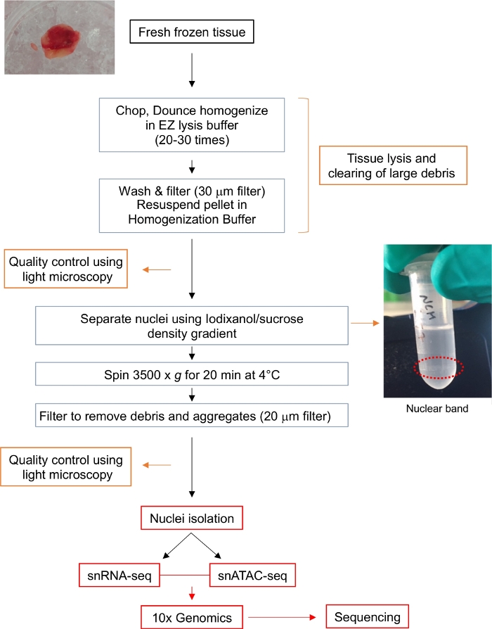
Figure 1: Flow chart for nuclei isolation. The flow chart provides a brief outlook on the steps involved in the isolation of single nuclei from a fresh frozen glioma tissue. Representative images for the tumor sample and the nuclear band after Iodixanol/sucrose gradient (circled with red dotted line) are shown. Please click here to view a larger version of this figure.

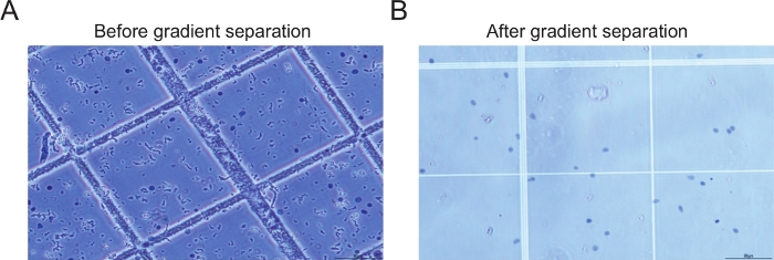
Figure 2: Examples of nuclei before and after gradient centrifugation. (A) The image of the sample before performing gradient centrifugation and filtration shows large amounts of debris (B) The image of the sample after gradient centrifugation and filtration step shows intact nuclei with minimal amount of debris. Please click here to view a larger version of this figure.

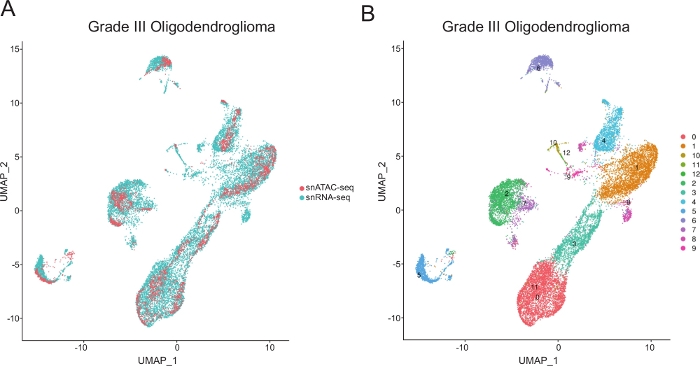
Figure 3: Example of co-embedded data from snRNA-seq and snATAC-seq using the same nuclei preparation. The Seurat R-statistical package was used to integrate the snRNA-seq and snATAC-seq data²⁷. (A) Co-embedded image of snRNA-seq and snATAC-seq data (B) Clusters produced by co-embedding of snRNA-seq and snATAC-seq data. Please click here to view a larger version of this figure.

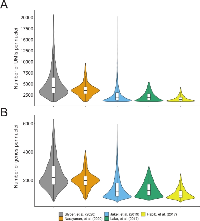
Figure 4: Quality control parameters of different human brain snRNA-seq datasets showing the individual number of UMI (A) and number of genes (B) per nuclei. The number of nuclei that passed quality filters were as follows: 3527 nuclei from the Slyper dataset, 14636 nuclei from the Narayanan dataset generated using the described protocol, 7369 nuclei from the Jakel dataset, 16494 nuclei from the Lake dataset, and 4652 nuclei from the Habib dataset. Please click here to view a larger version of this figure.

6x Homogenization Buffer Stable Master Mix
Reagent	Final Conc.	Vol for 100 (mL)
1 M CaCl2	30 mM	3.0
1 M Mg(Ac)2	18 mM	1.8
1 M Tris pH 7.8	60 mM	6.0
H2O		89.2
Keep at room temperature, avoid direct exposure to light

Table 1: Preparation of 6x Homogenization Buffer Stable Master Mix.

1 M Sucrose

34.23 g of sucrose

Dissolve in 78.5 mL of water

Fill up to 100 mL with water

Table 2: Preparation of 1 M sucrose.

6x Homogenization Buffer Unstable Solution (650 mL per sample)
Reagent	Final Conc.	Vol per sample (µL)
6x Homogenization Buffer Stable	6x	648.84
100 mM PMSF (Phenylmethylsulfonyl fluoride)	0.1 mM	1.08
14.3 M β-mercaptoethanol	1 mM	0.08

Table 3: Preparation of 6x Homogenization Buffer Unstable Solution (650 µL per sample).

1x Homogenization Buffer Unstable Solution (2 mL per sample)
Reagent	Final Conc.	Vol per sample (µL)
6x Homogenization Buffer Unstable	1x	333.33
1 M Sucrose	320 mM	640.00
50 mM EDTA	0,1 mM	4.00
10% NP40	0.1%	20.00
H2O		1006.27

Table 4: Preparation of 1x Homogenization Buffer Unstable Solution (2 mL per sample).

50% Iodixanol Solution (200 µL per sample)
Reagent	Final Conc.	Vol per sample (µL)
6x Homogenization Buffer Unstable	1x	66.67
60% Iodixanol Solution	50%	333.33

Table 5: Preparation of 50% Iodixanol Solution (200 µl per sample).

29% Iodixanol Solution (300 µL per sample)
Reagent	Final Conc.	Vol per sample (µL)
6x Homogenization Buffer Unstable	1x	100
1 M Sucrose	160 mM	96
60% Iodixanol Solution	29%	290
H2O		114

Table 6: Preparation of 29% Iodixanol Solution (300 µl per sample).

35% iodixanol Solution (300 µL per sample)
Reagent	Final Conc.	Vol per sample (µL)
6x Homogenization Buffer Unstable	1x	100
1 M Sucrose	160 mM	96
60% Iodixanol Solution	35%	350
H2O		54

Table 7: Preparation of 35% Iodixanol Solution (300 µl per sample).

Discussion

The field of intra-tumoral heterogeneity is at an exciting stage, with novel assays and platforms being developed to challenge and expand the existing knowledge. Intra-tumoral heterogeneity is a crucial factor that contributes to disease progression and resistance to current treatment modalities in gliomas²⁸. Recent studies on brain tumors have focused on this important aspect by using single cell transcriptomic and epigenomic assays to better characterize the cellular heterogeneity within the same tumor^29,30,31,32. One of the current bottlenecks with the single cell assays in brain tumors, and other solid tumors, is the availability of fresh clinical specimens. To overcome this problem, various studies have shown that using nuclei from fresh frozen tissues can be an alternative to fresh specimens and can be successfully used to interrogate cellular heterogeneity^18,33.

Here, we improve the previous single nuclei isolation methods in terms of simplicity, length, abundance, and quality of nuclei. This approach further brings the advantage of profiling snRNA-seq and snATAC-seq from the same nuclei preparation, allowing for multi-omics studies. In this procedure, we have modified existing protocols by adding an extra process of gradient separation using a non-ionic iodixanol-based medium. This approach allows for the isolation of pure nuclei without the need for FACS sorting, and the quality of the nuclei is assessed under a light microscope. A good quality suspension of nuclei should have no clumping, minimal debris, and intact nuclei. Although infrequent, clumping of nuclei can occur during the isolation step, which can be resolved by light pipetting using wide-bore P200 pipette tips or by straining the nuclei through a 20 mm filter. The most critical factor in single nucleus genomics is the ability to obtain pure and intact single nuclei. The presence of debris or aggregates can lead to a block of the microfluidic chambers within the single cell platforms, thereby leading to either low-quality data or to a possible failure of the experiment. The purpose of using filters at various steps followed by observation under a light microscope is to prevent such occurrences.

The amount and quality of starting material (e.g., fresh frozen tumor) are also important considerations. We have successfully used the protocol described here with brain tumor tissue blocks ranging from 10 mg to 60 mg. For these specimens, 500 µL of nuclei lysis buffer (Step 1) is sufficient to obtain sufficient good quality nuclei for single nuclei sequencing. Significantly larger tumor blocks that contain greater than 60-70% tumor content can be chopped into smaller pieces, and pieces can either be immediately placed back into liquid nitrogen or -80 °C storage or divided into tubes for single nuclei isolation and mixed once the lysis step is completed. In addition, tissue quality and tumor content should be assessed by Hematoxylin and Eosin (H&E) staining followed by confirmation from a pathologist.

The next important factors to consider are temperature and time of processing. Improper tissue storage, sample handling, and lengthy protocols can negatively impact the quality of the final genomics data. The samples need to be kept on ice, and the time for sample processing needs to be quick to prevent degradation of nuclei. The average processing for one sample with this protocol is 45-60 minutes, and it takes approximately 2 hours to process four samples. Improper tissue storage can also affect nuclei isolation and data quality. We assessed whether length of storage time at -80 °C impacted the quality of the data generated using the described protocol. The comparison of sequencing results obtained from the frozen samples banked between 1 to 14 years (2006-2019) showed no differences in data quality with respect to storage time. Therefore, properly frozen and stored fresh frozen tissue samples can be used for retrospective studies using this protocol.

There are several limitations with the single nuclei protocols. For example, different cell types cannot be sorted based on cell surface markers, and cytoplasmic transcripts are not detectable. Also, we omit the mitochondrial transcripts hence losing out on certain biological information related to tumor metabolism. Furthermore, different tissue types may require different lysis buffers thus requiring optimization of the protocol with each new experimental setup.

Overall, the protocol described here is simple, reduces sample processing time, and yields high-quality nuclei. The lack of a sorting step reduces stress on the nuclei and eliminates the need for a cell sorter. The absence of mitochondrial RNA increases the sequencing depth of nuclear transcripts. Importantly, similar to other single nuclei isolation protocols, this enhanced protocol facilitates the use of archived frozen specimens for retrospective analysis. We have successfully applied this workflow to perform snRNA-seq and snATAC-seq using the same nuclei preparation from brain tumors without the need to change buffers. Therefore, this approach allows for multi-omics studies from the same specimen.

In conclusion, the single nuclei isolation method described here is a highly effective, accurate and rapid technique which can be applied to perform single-nucleus sequencing studies.

Materials

List of materials used in this article

Name	Company	Catalog Number	Comments
2-Mercaptoethanol	Sigma	M6250
CaCl2	Sigma	21115-100ML
Dounce Homogenizer	Active motif	40401
EDTA (0.5 M)	Thermo Scientific	R1021
Falcon 15 mL Conical Centrifuge Tubes	Fisher Scientific	352096
Iodixanol (aka Optiprep)	Stem cell technologies	07820
MACs Smart Strainers (30 µm)	Miltenyi Biotec	130-098-458
MACS SmartStrainers (100 µm)	Miltenyi Biotec	130-098-463
Mg(Ac)2	Sigma	63052-100ML
NP-40	Abcam	ab142227
Nuclei Isolation Kit: Nuclei EZ Prep	Sigma	NUC101-1KT
Phenylmethanesulfonyl fluoride (PMSF)	Sigma	P7626
Pre-Separation Filters (20 µm)	Miltenyi Biotec	130-101-812
Safe lock tubes 1.5 mL	Eppendorf	0030120086
Safe lock tubes 2.0 mL	Eppendorf	0030120094
Single Cell ATAC	10x Genomics
Single Cell Gene Expression	10x Genomics
Sucrose	Sigma	S0389
Wide Bore pipette tips (1000 µL)	Themo Fisher Scientific	2079GPK
Wide Bore pipette tips (200 µL)	Themo Fisher Scientific	2069GPK

References

- Huse, J. T., Holland, E. C. Targeting brain cancer: advances in the molecular pathology of malignant glioma and medulloblastoma. Nature Reviews Cancer. 10 (5), 319-331 (2010).
- Kreso, A., Dick, J. E. Evolution of the cancer stem cell model. Cell Stem Cell. 14 (3), 275-291 (2014).
- Filbin, M. G., Suva, M. L. Gliomas Genomics and Epigenomics: Arriving at the Start and Knowing It for the First Time. Annual Review of Pathology. 11, 497-521 (2016).
- Ferris, S. P., Hofmann, J. W., Solomon, D. A., Perry, A. Characterization of gliomas: from morphology to molecules. Virchows Archive. 471 (2), 257-269 (2017).
- Louis, D. N., et al. The 2016 World Health Organization Classification of Tumors of the Central Nervous System: a summary. Acta Neuropathologica. 131 (6), 803-820 (2016).
- Eckel-Passow, J. E., et al. Glioma Groups Based on 1p/19q, IDH, and TERT Promoter Mutations in Tumors. The New England Journal of Medicine. 372 (26), 2499-2508 (2015).
- Suzuki, H., et al. Mutational landscape and clonal architecture in grade II and III gliomas. Nature Genetics. 47 (5), 458-468 (2015).
- Cancer Genome Atlas Research. Comprehensive, Integrative Genomic Analysis of Diffuse Lower-Grade Gliomas. The New England Journal of Medicine. 372 (26), 2481-2498 (2015).
- Noushmehr, H., et al. Identification of a CpG island methylator phenotype that defines a distinct subgroup of glioma. Cancer Cell. 17 (5), 510-522 (2010).
- Yan, H., et al. IDH1 and IDH2 mutations in gliomas. The New England Journal of Medicine. 360 (8), 765-773 (2009).
- Yan, H., Bigner, D. D., Velculescu, V., Parsons, D. W. Mutant metabolic enzymes are at the origin of gliomas. Cancer Research. 69 (24), 9157-9159 (2009).
- Gawad, C., Koh, W., Quake, S. R. Single-cell genome sequencing: current state of the science. Nature Reviews Genetics. 17 (3), 175-188 (2016).
- Tanay, A., Regev, A. Scaling single-cell genomics from phenomenology to mechanism. Nature. 541 (7637), 331-338 (2017).
- Wu, M., Singh, A. K. Microfluidic Flow Cytometry for Single-Cell Protein Analysis. Methods in Molecular Biology. 1346, 69-83 (2015).
- Schwartzman, O., Tanay, A. Single-cell epigenomics: techniques and emerging applications. Nature Reviews Genetics. 16 (12), 716-726 (2015).
- Macaulay, I. C., Ponting, C. P., Voet, T. Single-Cell Multiomics: Multiple Measurements from Single Cells. Trends in Genetics. 33 (2), 155-168 (2017).
- Buenrostro, J. D., et al. Single-cell chromatin accessibility reveals principles of regulatory variation. Nature. 523 (7561), 486-490 (2015).
- Habib, N., et al. Massively parallel single-nucleus RNA-seq with DroNc-seq. Nature Methods. 14 (10), 955-958 (2017).
- Corces, M. R., et al. An improved ATAC-seq protocol reduces background and enables interrogation of frozen tissues. Nature Methods. 14 (10), 959-962 (2017).
- Slyper, M., et al. A single-cell and single-nucleus RNA-Seq toolbox for fresh and frozen human tumors. Nature Medicine. 26 (5), 792-802 (2020).
- Mathys, H., et al. Single-cell transcriptomic analysis of Alzheimer's disease. Nature. 570 (7761), 332-337 (2019).
- Krishnaswami, S. R., et al. Using single nuclei for RNA-seq to capture the transcriptome of postmortem neurons. Nature Protocols. 11 (3), 499-524 (2016).
- Al-Dalahmah, O., et al. Single-nucleus RNA-seq identifies Huntington disease astrocyte states. Acta Neuropathologica Communications. 8 (1), 19(2020).
- Jakel, S., et al. Altered human oligodendrocyte heterogeneity in multiple sclerosis. Nature. 566 (7745), 543-547 (2019).
- Butler, A., Hoffman, P., Smibert, P., Papalexi, E., Satija, R. Integrating single-cell transcriptomic data across different conditions, technologies, and species. Nature Biotechnology. , (2018).
- Lake, B. B., et al. Integrative single-cell analysis of transcriptional and epigenetic states in the human adult brain. Nature Biotechnology. 36 (1), 70-80 (2018).
- Stuart, T., et al. Comprehensive Integration of Single-Cell Data. Cell. 177 (7), 1888-1902 (2019).
- Bready, D., Placantonakis, D. G. Molecular Pathogenesis of Low-Grade Glioma. Neurosurgery Clinics of North America. 30 (1), 17-25 (2019).
- Venteicher, A. S., et al. Decoupling genetics, lineages, and microenvironment in IDH-mutant gliomas by single-cell RNA-seq. Science. 355 (6332), (2017).
- Tirosh, I., et al. Single-cell RNA-seq supports a developmental hierarchy in human oligodendroglioma. Nature. 539 (7628), 309-313 (2016).
- Weng, Q., et al. Single-Cell Transcriptomics Uncovers Glial Progenitor Diversity and Cell Fate Determinants during Development and Gliomagenesis. Cell Stem Cell. 24 (5), 707-723 (2019).
- Neftel, C., et al. An Integrative Model of Cellular States, Plasticity, and Genetics for Glioblastoma. Cell. 178 (4), 835-849 (2019).
- Al-Ali, R., et al. Single-nucleus chromatin accessibility reveals intratumoral epigenetic heterogeneity in IDH1 mutant gliomas. Acta Neuropathologica Communications. 7 (1), 201(2019).
Reprints and Permissions