Use of 3D Robotic Ultrasound for In Vivo Analysis of Mouse Kidneys

Summary

This protocol demonstrates robotic ultrasound (US) as a practical, cost-effective, and quick alternative to traditional non-invasive image modalities.

Abstract

Common modalities for in vivo imaging of rodents include positron emission tomography (PET), computed tomography (CT), magnetic resonance imaging (MRI), and ultrasound (US). Each method has limitations and advantages, including availability, ease of use, cost, size, and the use of ionizing radiation or magnetic fields. This protocol describes the use of 3D robotic US for in vivo imaging of rodent kidneys and heart, subsequent data analysis, and possible research applications. Practical applications of robotic US are the quantification of total kidney volume (TKV), as well as the measurement of cysts, tumors, and vasculature. Although the resolution is not as high as other modalities, robotic US allows for more practical high throughput data collection. Furthermore, using US M-mode imaging, cardiac function may be quantified. Since the kidneys receive 20%-25% of the cardiac output, assessing cardiac function is critical to the understanding of kidney physiology and pathophysiology.

Introduction

The most common modalities for in vivo rodent imaging include positron emission tomography (PET), optical imaging (OI), computed tomography (CT), magnetic resonance imaging (MRI), and ultrasound (US). These techniques provide high-resolution in vivo images, allowing investigators to quantitatively assess and longitudinally follow disease models non-invasively¹. While each imaging modality has limitations, they also provide invaluable tools for preclinical research.

Here, the study details a US system and presents the protocol for robotic and 3D rodent imaging. US waves are produced by a probe called a transducer, which is typically hand-held. Sound waves are reflected back as they interact with tissues, and the echoes are reconstructed into images². The protocol described here will focus on kidney and cardiac imaging using a robotically controlled transducer and using software that allows rapid 3D reconstruction for quantitative assessment.

Robotic US is a fast, reliable, and non-invasive imaging modality that allows investigators to conduct high-throughput and longitudinal studies. Compared to hand-held US methods, the robotic US method is time-efficient, as up to three animals can be scanned in a matter of minutes. High throughput for kidney measurements suggests that up to 20 mice per hour may be imaged. The robotic transducers are located underneath the acoustic membranes and move independently of the animal with two degrees of freedom (Figure 1A). This allows novice users to obtain high-quality images, whereas hand-held US methods are more susceptible to user error. The coupled software allows efficient, real-time 3D kidney reconstruction. Previously, magnetic resonance imaging (MRI) has been a prevalent method for non-invasive imaging due to the excellent soft-tissue contrast, lack of radioactivity, and penetration depth. However, MRI often requires long acquisition times and is costly to perform. US has been evaluated as a reliable and more rapid alternative to MRI in assessing total kidney volume (TKV)³.

Protocol

All steps in this protocol comply with the Mayo Clinic (Rochester, MN) animals use guidelines and have been approved by the Mayo Clinic Institutional Animal Care and Use Committee.

1. Animal model

1. Obtain mice from commercial sources.
   ​NOTE: C57BL/6J (age = 18 months; n = 22 (7 males, 15 females)) (Table of Materials) and Pkd1^(RC/RC) (age = 18 months; n = 9 (3 males, 6 females))⁴ were used for the study.

2. Hair removal

1. Anesthetize the animal using vaporized isoflurane (2%-3%) in an anesthesia chamber. Ensure that the animal is sufficiently anesthetized by performing a toe pinch. Ensure that the mouse is breathing at a rate of approximately 60-90 breaths/min without obvious air gulping.
   NOTE: Vaporized isoflurane was chosen due to the ability to control and fine-tune the animal's level of anesthesia. Isoflurane mixed with 100% oxygen was utilized.
2. Use an electric razor to shave the desired skin area for US measurements.
   NOTE: In this study, the focus is on kidney and cardiac measurements, so the animal's chest and back were shaved.
3. Apply the depilatory cream to the animal's shaved skin with a cotton-tipped applicator. Wipe the cream off after 30-60 s using a dry paper towel. Then, continue to wipe away depilatory cream residue using wet gauze pads. Ensure the hair removal is complete prior to beginning scans.
   ​NOTE: Any remaining hair will interfere with the image quality; complete hair removal is crucial. However, it is necessary to wipe the depilatory cream off within a minute to prevent injuring the animal's skin. Leftover depilatory cream on the animal can stain the imaging membrane of the US machine. Ensure proper cleaning of the animal using wet gauze pads.

3. Animal positioning

1. Turn on the US machine and the switch for the internal heating element for the US bays. Turn on the appropriate anesthesia valves for the corresponding US bays that will be used.
   NOTE: The US machine must be turned on prior to starting the imaging US software.
2. Fill the bays with enough water to cover the membrane. Place the anesthetized animal in the nose cone.
   1. For cardiac measurements, place the animal in a prone position and angle it approximately 30° to the right.
   2. For kidney measurements, place the animal in a straight and supine position. Gently flatten the animal's body to minimize the air pockets between the animal and the membrane (Figure 1B).
      NOTE: Running a finger alongside the animal's body can remove any air bubbles adhering to the skin, which will interfere with imaging. Use water or US saline gel as US medium; but water facilitates the rapid imaging discussed here.

4. Ultrasound measurements

1. In the imaging US software, select US Acquisition and allow the instrument to initialize.
2. Kidney Imaging using B-mode.
   1. Enter a name for the study in the appropriate dialog box.
   2. Enter the animal ID in the appropriate dialog box.
      ​NOTE: Up to three animals can be imaged sequentially.
   3. Click on the tab labeled 3D to initialize 3D scanning.
   4. Using the live camera feed, move the region of interest (ROI) box to contain the kidneys.
      NOTE: The size of the ROI may be adjusted depending on the size of the image target. Increasing the size of the ROI will slightly increase the scan time (Figure 1C). Depending on ROI size, the scanner will automatically adjust the number of passes required for the transducer to scan the entire ROI.
   5. Depending on the type of image desired, select Linear Array or Wobbler, to choose the transducer. Select from Fast Scan or Optimized for either transducer.
      NOTE: Linear array is faster and usually provides adequate imaging. The wobbler transducer can be utilized if unable to acquire the desired image quality with the linear array. The wobbler transducer utilizes a higher frequency wavelength and therefore provides more definition in images. The Fast Scan option acquires medium quality images with no breathing correction at a higher speed. While the Optimized option requires slightly more time, it provides better image quality and allows for breathing correction. This manuscript will focus on using the Optimized linear array preset.
   6. Click on the Live View to see a live image of the desired viewing area.
   7. To move the transducer, click on the circular Go To button, and then click on the area of the mouse to be imaged. Use the directional arrows with predetermined step sizes to finely adjust the transducer position.
   8. Click on the arrow at the side of the Control Panel window to open the Settings Tray. Click on Scan Protocol to open scanning settings.
   9. Determine the ideal focal depth and adjust the sliders for the TGC (time gain compensation) to change the image contrast to best view the kidneys. After achieving the desired settings, click on the arrow again to close the Settings Tray.
   10. Press the Acquire Static button to commence 3D scanning.
       NOTE: Progress of the scan is indicated via a progress bar in the bottom left of the software.
   11. Once the scanning is complete, check the image quality by clicking on the blue download arrow to open the scan in Preview Mode. Move through the 3D frames of the scan by dragging the red arrow at the top of the window. To zoom in or out, hold the Ctrl key and use the scroll button on the mouse.
   12. To scan additional animals, refresh the animal ID dialog boxes, input the new IDs, and then repeat the above steps.
       NOTE: When the scans are complete, dry the animals off and return them to their home cages.
3. Cardiac imaging using M mode.
   NOTE: M-mode is the display of an ultrasound wave along a specific, chosen ultrasound line.
   1. Click on the M Mode tab to activate cardiac imaging.
      ​NOTE: Only one animal can be imaged at a time.
   2. Ensure that the animal is in the appropriate position for cardiac scans (step 2.2). Move the ROI to the approximate location of the heart.
   3. Push the Heart Finder button to locate the heart. Use the heat map to optimize the location of the transducer. Use the circular Go To button to move the transducer to the left ventricle (Figure 2A).
   4. Go to the Live View and use the arrow buttons to place the transducer between the papillary muscles (Figure 2B). To verify the proper placement of the transducer, view the live M Mode trace (Figure 2D).
   5. Once the transducer is in the appropriate position, click on Acquire Sequence. Click on the blue download arrow to view the completed scan.

5. Kidney analysis (mechanics of analysis)

1. Open the Image Analysis tab and select the Load Volume(s) button to input the image files/folders.
   1. Segmentation
      1. Move the colored lines representing various planes to find the kidney in all the planes.
      2. Click on Add to add a new segmentation. Provide a markup name for the file.
      3. Use the Surface Cut button to add points around the outer edge of the kidney in multiple planes. Click on Apply to generate segmentation through the entire kidney (Figure 3A).
      4. Scroll through the different frames in each plane and edit any inaccurate regions by clicking on Edit and dragging the points to the correct location.
      5. Alternatively, if the kidney is irregular in shape, use the Draw function to create an irregularly shaped trace around the kidney. Either click points around the edge or hold the left click to draw the trace freehand.
      6. To complete the trace with the Draw button, right-click with the mouse. Scroll ahead multiple frames and repeat the tracing process.
      7. Repeat until the frames are traced throughout the entire region of interest.
      8. If the Draw function is used, select Fill Between Slices to check and adjust the trace. Click on Initialize to see a preview. If the preview is acceptable, click on Apply. If not, click on Cancel and modify the tracings.
         NOTE: The Erase button will allow deletion of a region within a trace. The Smooth button smooths the jagged edges of a trace.
      9. When image analysis is satisfactory, select Save to save the analysis to the original image file.
   2. Measurement
      1. Use the Calipers function to measure features within the image. Click on the Calipers button and left click the two points of the distance to be measured (Figure 3B).
      2. Save the measurement by clicking the disk button at the top of the screen.

6. Cardiac analysis

1. Select Load Volumes to input the file(s) to analyze.
2. Select the Add option.
3. Use the Point Placement tool to trace the systole and diastole for each layer of heart tissue. Continue with the other layers of heart tissue. Use the Edit function to modify the traces (Figure 2C,D).
   NOTE: If the M-mode trace is very clear, use the Add (auto) button to automatically generate tracings of each layer.
4. Select Apply to calculate the cardiac parameters. View the Quantify tab and select Export Statistics to export all data as a *.csv file (Figure 2E).

Results

Results of kidney analysis
Surface area and volume data are acquired from the segmentation of the kidneys. This information can be used to compare experimental and control models or track changes over time. The calipers tool is useful for quickly measuring abnormalities (i.e., cysts, tumors) and how they change in length over time. Figure 3 suggests that both the segmentation and caliper methods can be used to measure cyst volumes accurately. Figure 4 demonstrates a clear difference in total kidney volume (TKV) between age-matched control and experimental (Pkd1^RC/RC) mice. 3D visualization of these volume renderings may be performed within the system, including rotations within 3D space (Figure 5). These 3D-reconstructions are then used to calculate TKV (mm³; Figure 4) as well as individual large cyst volume.

Results of cardiac analysis
Many useful parameters are acquired from the analysis of M Mode images. These data provide a good snapshot of the left ventricular (LV) cardiac function at that point in time. The data output includes LV internal diameter, LV posterior wall, LV anterior wall diameter, ejection fraction, fractional shortening, stroke volume, heart rate, cardiac output, LV volume, and LV mass. The success of cardiac analysis is dependent on accurate segmentation of the layers on the M Mode image. Most cardiovascular results are calculated by the peak systolic and diastolic phases of the posterior and anterior endocardial layers. The posterior epicardial layer appears bright white and follows a similar pattern to the posterior endocardial layer. The tracing for the posterior endocardial layer should be placed on the lowest contour. The anterior endocardial layer should be traced along the highest contour of that layer. The anterior epicardial layer appears linear at the bottom of the image due to the prone positioning of the animal (Figure 2D). Figure 6 shows an example of one study with no significant difference in cardiac output between experimental and control mice. As with renal imaging, 3D cardiac visualization is possible. Nevertheless, a 4D visualization of the cardiac cycle (Supplemental Figure 1) allows the investigator to visualize and pinpoint both morphologic and cycle-dynamic abnormalities in the assessed animal.

Morphology assessment
For quick and inexpensive assessment, US can effectively monitor physiological parameters longitudinally. However, many studies wish to additionally determine finer morphologic characteristics, e.g., number and sizes of cysts, calcifications (kidney stones), vascularization, or degree of fibrosis. Figure 7 compares a normal mouse kidney to a cystic mouse kidney to a moderately calcified mouse kidney. By increasing the US center frequency (10 MHz with the linear array) to 35 MHz (wobbler amplifier), pictures of increasing detail may be obtained.

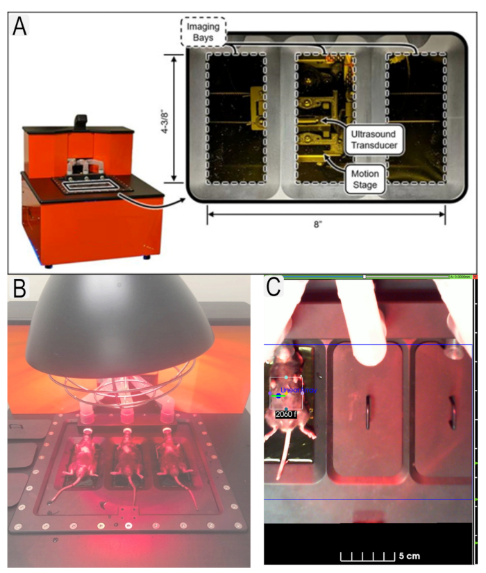
Figure 1: Ultrasound system and mouse placement. (A) Diagram of ultrasound system and location of transducers. (B) View of mice in supine position on ultrasound platform. (C) Example of region of interest (ROI)s in place for area of interest (kidneys) with animal IDs. Please click here to view a larger version of this figure.

Figure 2: Cardiac ultrasound imaging to obtain physiological parameters. (A) Use of the Heart Finder heatmap image to position the transducer in the left ventricle for M-Mode imaging. The transducer location in the left ventricle is indicated by the large green dot. (B) View of the transducer when placed correctly over papillary muscles (dotted box). (C) Example view of layers needed to measure cardiac parameters. (D) View of live M-Mode image with layers designated as in panel C. (Layers from top to bottom: posterior epicardial, posterior endocardial, anterior endocardial, and anterior epicardial.) (E) Example output of statistics generated from cardiac measurements. Please click here to view a larger version of this figure.

Figure 3: Using segmentation and calipers tools to measure kidneys and cyst. (A) Example segmentations (axial view) of both kidneys (blue and orange shading) and a large cyst (yellow) with volumes listed below. Non-segmented views are shown underneath so that the unobscured US may be viewed. (B) Example use of calipers to measure the same cyst (sagittal view) from Figure 3A with measurements below. The volume was calculated using the formula for an ellipse (volume = (4/3)π x a x b x c, where a, b, c are relative x, y, z, respectively). Please click here to view a larger version of this figure.

Figure 4: TKV distributions of WT and cystic mouse kidneys. Representation of TKVs for wild-type (WT) (C57BL/6J) and diseased (Pkd1^RC/RC) mice. n = 22 (WT) n = 9 (Pkd1^RC/RC); Results of two-tailed t-test: p < 0.0001. Box shows 25-75^th percentile values and whiskers show 1.5 times interquartile range. Please click here to view a larger version of this figure.

Figure 5: Animated 3D reconstruction of segmented kidneys and cyst. Using the software, the 3D projections of the kidneys and cyst may be rotated or rocked in the 3D space (blue = left kidney; yellow = large cyst; orange = right kidney). Please click here to download this figure.

Figure 6: Cardiac physiological parameters from US measurements. Representation of cardiac output (mL/min) for WT and diseased (Pkd1^RC/RC) mice. n = 22 (WT) n = 9 (Pkd1^RC/RC). The lower tabulated data show that there is no significant difference for these two groups in ejection fraction, stroke volume, heart rate (HR), or cardiac output (CO). Results of two-tailed t-test: p > 0.05. Box shows 25-75^th percentile values. Please click here to view a larger version of this figure.

Figure 7: Comparison of US sagittal sections of normal and two pathologies. (A) Wild-type (C57BL/6J strain) kidney (TKV = 143.202 mm³). (B) Cystic kidney with increased TKV (Pkd1^RC/RC mouse) (TKV = 333.158 mm³). Cysts are indicated by yellow arrows. (C) Kidney with vascular calcifications (Model = Low-Density Lipoprotein Receptor Deficient, Apolipoprotein B100-only mouse fed a Western diet for 12 months⁵) (TKV = 127.376 mm³). Renal stones are indicated by green arrows. Please click here to view a larger version of this figure.

Supplemental Figure 1: 4D cardiac cycle movie from US measurements. Using the software, a representation of the beating heart is captured in 3D US and projected through the cardiac cycle. The green arrow indicates the aortic valve. (Model = Low-Density Lipoprotein Receptor Deficient, Apolipoprotein B100-only mouse, fed a Western diet for 12 months⁵). This model generates vascular calcifications enabling easier visualization of the heart and valves due to the greater acoustic reflectivity of the calcifications in US. Similar 4D reconstructions are possible with WT mice; however, the captured acoustic contrast will not be as high. Please click here to download this File.

Discussion

Ultrasound utilizes sound waves, and any barriers to sound wave propagation will interfere with image quality. Thus, complete hair removal of the area to be imaged is critical. It is also important to ensure complete removal of depilatory cream as it can cause burns/irritation of the animal's skin and discolor the transparent membrane of the scanner. Adequate water levels in the bays are necessary for optimal sound wave propagation, thus required for obtaining the highest image resolution. However, when the animal is in a prone position, ensure the animal's snout is above the water level or the animal is at risk of water inhalation. Optimization of imaging parameters, especially focal depth, is critical for obtaining high-quality images. Modifications to parameters may be necessary for individual animals.

Robotic US provides many advantages over traditional hand-held US modalities. First, the system uses a simple point-and-click camera-based interface. This feature addresses the complexity of conventional US and produces consistent data even when operated by a novice user⁶. Second, the system allows the use of water rather than traditional US gel as an acoustic medium. Previously, the use of US gel allowed the formation of bubbles that interfered with quality image acquisition. Also, the US gel is messy and provides challenges for clean-up. Further, the water is warmed by the heat lamp and helps maintain the animal's body temperature. Third, the robotic US is faster, so artifacts from respiratory motion are not problematic. The increased imaging speed allows for the practical completion of high throughput data collection. Fourth, the robotic US obtains 3D images, and therefore makes 3D reconstruction of objects simple (Figure 4). MRI and other modalities are expensive, time-consuming, and not always available. Importantly, the robotic US system fits on a table or bench and is more cost-efficient. Finally, prior work demonstrated that robotic US could provide comparable measurement data to more expensive modalities, such as MRI³.

While the image quality and resolution of the robotic US system described in this work were adequate for the proposed application (Figure 7), there are several ways that image quality can be improved in the future. For instance, utilizing higher frequency transducers (e.g., 50-70 MHz) would result in higher resolution images with better feature definition. While utilizing higher frequencies would result in a poorer depth of penetration, the images should be sufficient for in vivo imaging of superficial organs, such as the mouse kidney. As with other imaging modalities, contrast agents may be used to enhance specific features. For US, this typically means using something highly reflective of sound waves. Intravascular microbubbles in which lipids surround very small gas bubbles are one such agent. The micron-sized gas bubbles are highly reflective and thus provide a second distinct signal that translates into a high-resolution of vasculature⁷. While this acoustic contrast technique may be quite useful, it can have several downsides. First, the microbubbles must be made fresh and only persist in vivo for 5-10 min. Second, in vivo intravascular injection typically requires tail veil catheterization for injection, and this can be technically challenging. Under certain circumstances and pulsing regimes, microbubble imaging can itself lead to renal vasculature damage⁸.

There are also some more general limitations of the particular US system used. First, only one linear array (centered at 18 MHz) is included in the robotic chassis, so switching to higher or lower frequency probes is not currently possible. This may impact the breadth of models (either larger or smaller) that can be evaluated with the system. Future iterations of the instrument should include multiple linear arrays to cover the full range of preclinical animal models. Second, the transducer angle relative to the animal subject cannot be controlled. Therefore, performing angle-dependent imaging techniques, such as Doppler, or achieving alternative in-plane views of certain organs (e.g., long axis view of kidney) requires repositioning of the animal and can be difficult to achieve. Additional degrees-of-freedom could be added to the robotic movement to ameliorate this challenge. Third, on occasion, we have observed reverberation artifacts arising from the acoustic membrane that separates the animal from the transducer that can obscure visualization of superficial features and boundaries. In these cases, using a gel standoff to elevate the animal away from the membrane can remedy the situation. Finally, temperature control via heat lamp is imprecise, and therefore close attention must be paid to the animal's core body temperature while imaging. More controlled heating mechanisms, such as an integrated heating pad, will likely improve homeostasis management and imaging throughput.

The use of robotic US may be applicable to various fields of research. This technology enables visualization of gross tissue structures, thus may be used to track tumor progression and potential therapies^6,9 as well as renal morphology as presented here. The ability to segment the specific features of the images makes it an attractive tool for studying models of polycystic kidney disease (PKD)³. M-mode images allow for simple quantification of many important cardiac parameters enabling in vivo assessment of cardiac physiology. As the kidneys receive 20%-25% of the cardiac output¹⁰, understanding cardiac function during the longitudinal assessment of renal pathology is important. Through these US protocols, we have tried to illustrate that US imaging is not only practical for in vivo and longitudinal kidney studies but also that increasingly US tools enable both morphologic as well as physiologic assessment of mice in preclinical studies.

Materials

List of materials used in this article

Name	Company	Catalog Number	Comments
Electric Razor	Braintree Scientific, Inc	CLP-9868 14
C57bk6j	The Jackson laboratory		https://www.jax.org/
Cotton gauze pads	Fisher Scientific
Cotton tipped applicators	Fisher Scientific
Depilatory cream	N/a	N/a	This study used Nair
Heat lamp			Included with SonoVol Vega system
Robotic Ultrasound System	SonoVol Inc		SonoVol Vega system includes anesthesia system
SonoEQ Software	SonoVol		Included with SonoVol Vega system
TERRELL Isoflurane	Piramal Critical Care, Inc	NDC 66794-019-10