Computational Modeling of Retinal Neurons for Visual Prosthesis Research - Fundamental Approaches

Summary

We summarize a workflow to computationally model a retinal neuron's behaviors in response to electrical stimulation. The computational model is versatile and includes automation steps that are useful in simulating a range of physiological scenarios and anticipating the outcomes of future in vivo/in vitro studies.

Abstract

Computational modeling has become an increasingly important method in neural engineering due to its capacity to predict behaviors of in vivo and in vitro systems. This has the key advantage of minimizing the number of animals required in a given study by providing an often very precise prediction of physiological outcomes. In the field of visual prosthesis, computational modeling has an array of practical applications, including informing the design of an implantable electrode array and prediction of visual percepts that may be elicited through the delivery of electrical impulses from the said array. Some models described in the literature combine a three-dimensional (3D) morphology to compute the electric field and a cable model of the neuron or neural network of interest. To increase the accessibility of this two-step method to researchers who may have limited prior experience in computational modeling, we provide a video of the fundamental approaches to be taken in order to construct a computational model and utilize it in predicting the physiological and psychophysical outcomes of stimulation protocols deployed via a visual prosthesis. The guide comprises the steps to build a 3D model in a finite element modeling (FEM) software, the construction of a retinal ganglion cell model in a multi-compartmental neuron computational software, followed by the amalgamation of the two. A finite element modeling software to numerically solve physical equations would be used to solve electric field distribution in the electrical stimulations of tissue. Then, specialized software to simulate the electrical activities of a neural cell or network was used. To follow this tutorial, familiarity with the working principle of a neuroprosthesis, as well as neurophysiological concepts (e.g., action potential mechanism and an understanding of the Hodgkin-Huxley model), would be required.

Introduction

Visual neuroprostheses are a group of devices that deliver stimulations (electrical, light, etc.) to the neural cells in the visual pathway to create phosphenes or sensation of seeing the light. It is a treatment strategy that has been in clinical use for almost a decade for people with permanent blindness caused by degenerative retinal diseases. Typically, a complete system would include an external camera that captures the visual information around the user, a power supply and computing unit to process and translate the image to a series of electrical pulses, and an implanted electrode array that interfaces the neural tissue and deliver the electrical pulses to the neural cells. The working principle allows a visual neuroprosthesis to be placed in different sites along the visual pathway from the retina to the visual cortex, as long as it is downstream from the damaged tissue. A majority of current research in visual neuroprostheses focuses on increasing the efficacy of the stimulation and improving the spatial acuity to provide a more natural vision.

In the efforts to improve the efficacy of the stimulation, computational modeling has been a cost- and time-effective method to validate a prosthesis design and simulate its visual outcome. Computational modeling in this field gained popularity since 1999 as Greenberg¹ modeled the response of a retinal ganglion cell to extracellular electrical stimuli. Since then, computational modeling has been used to optimize the parameters of the electrical pulse^2,3 or the geometrical design of the electrode^4,5. Despite the variation in complexity and research questions, these models work by determining the electrical voltage distribution in the medium (e.g., neural tissue) and estimating the electrical response that the neurons in the vicinity will produce due to the electrical voltage.

The electrical voltage distribution in a conductor can be found by solving the Poisson equations⁶ at all locations:

where E is the electric field, V the electric potential, J the current density, and σ is the electrical conductivity. The in the equation indicates a gradient operator. In the case of stationary current, the following boundary conditions are imposed on the model:

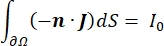
where n is the normal to the surface, Ω represents the boundary, and I₀ represents the specific current. Together, they create electrical insulation at the external boundaries and create a current source for a selected boundary. If we assume a monopolar point source in a homogeneous medium with an isotropic conductivity, the extracellular electric potential at an arbitrary location can be calculated by⁷:

where I_e is the current and is the distance between the electrode and the point of measurement. When the medium is inhomogeneous or anisotropic, or the electrode array has multiple electrodes, a computational suite to numerically solve the equations can be convenient. A finite-element modeling software⁶ breaks up the volume conductor into small sections known as 'elements'. The elements are interconnected with each other such that the effects of change in one element influence change in others, and it solves the physical equations that serve to describe these elements. With the increasing computational speed of modern computers, this process can be completed within seconds. Once the electric potential is calculated, one can then estimate the electrical response of the neuron.

A neuron sends and receives information in the form of electrical signals. Such signals come in two forms - graded potentials and action potentials. Graded potentials are temporary changes to the membrane potential wherein the voltage across the membrane becomes more positive (depolarization) or negative (hyperpolarization). Graded potentials typically have localized effects. In cells that produce them, action potentials are all-or-nothing responses that can travel long distances along the length of an axon. Both graded and action potentials are sensitive to the electrical as well as the chemical environment. An action potential spike can be produced by various neuronal cell types, including the retinal ganglion cells, when a threshold transmembrane potential is crossed. The action potential spiking and propagation then trigger synaptic transmission of signals to downstream neurons. A neuron can be modeled as a cable that is divided into cylindrical segments, where each segment has capacitance and resistance due to the lipid bilayer membrane⁸. A neuron computational programme⁹ can estimate the electrical activity of an electrically-excitable cell by discretizing the cell into multiple compartments and solving the mathematical model¹⁰:

In this equation, C_m is the membrane capacitance, V_e,n is the extracellular potential at node n, V_i,n the intracellular potential at node n, R_n the intracellular (longitudinal) resistance at node n, and I_ion is the ionic current going through the ion channels at node n. The values of V from the FEM model are implemented as V_e,n for all nodes in the neuron when the stimulation is active.

The transmembrane currents from ion channels can be modeled by using Hodgkin-Huxley formulations¹¹:

where g_i is the specific conductance of the channel, V_m the transmembrane potential (V_i,n - V_e,n) and E_ion the reversal potential of the ion channel. For voltage-gated channels, such as Na channel, dimensionless parameters, m, and h, that describe the probability of opening or closing of the channels are introduced:

where is the maximum membrane conductance for the particular ion channel, and the values of parameters m and h are defined by differential equations:

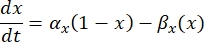
where α_x and β_x are voltage-dependent functions that define the rate constants of the ion channel. They generally take the form:

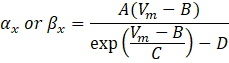
The values of the parameters in these equations, including maximal conductance, as well as the constants A, B, C, and D, were typically found from empirical measurements.

With these building blocks, models of different complexities can be built by following the steps described. An FEM software is useful when the Poisson equation cannot be solved analytically, such as in the case of inhomogeneous or anisotropic conductance in the volume conductor or when the geometry of the electrode array is complex. After the extracellular potential values have been solved, the neuron cable model can then be numerically solved in the neuron computational software. Combining the two software enables the computation of a complex neuron cell or network to a non-uniform electric field.

A simple two-step model of a retinal ganglion cell under a suprachoroidal stimulation will be built using the aforementioned programs. In this study, the retinal ganglion cell will be subjected to a range of magnitudes of electrical current pulses. The location of the cell relative to the stimulus is also varied to show the distance-threshold relationship. Moreover, the study includes a validation of the computational result against an in vivo study of the cortical activation threshold using different sizes of stimulation electrode¹², as well as an in vitro study showing the relationship between the electrode-neuron distance and the activation threshold¹³.

Protocol

1. Setting up the finite element model for electric potential calculations

1. Determine the simulation steps and the complexity of the model
   NOTE: The aim of the first step is to clarify the purpose of the modeling, which will determine the necessary elements of the model and the simulation procedure. An important point to consider is the behavior of neural cells that needs to be shown by the model, and what testing protocol would be needed to demonstrate that behavior. This study shows a distance-threshold relationship for a neuron that is extracellularly stimulated, as well as the electrode size-threshold curve. To do this, a neural cell model compartmentalized to different sections (to incorporate the variation of morphological and biophysical parameters in the neuron) sensitive to extracellular voltage and simulation of a range of electrode sizes and positions are needed.
   1. Define the research question and the experimental variables.
      1. Define a research question and testing protocol to guide the construction of the model. It is best to start with a clear question and build a model as simple as possible to answer it.
   2. Determine the necessary elements to be included in the complete model
      NOTE: In this modeling approach, the cell is seen as being immersed in an electrically conductive medium, that is, the biological tissue. The electrical stimulation happens across this 'volume conductor,' i.e., the medium, resulting in a distribution of electric potential.
      1. Based on the research questions and variables to solve, decide whether both elements (FEM and neuron cable model) are required. If, for example, the modeling needs a single electrode that can be simplified as a point source and that the medium is homogeneous, a FEM might not be necessary, and an analytical calculation of the extracellular electric field can be done to replace it.
2. Download and install the software
   NOTE: The study used the versions of software applications (COMSOL, NEURON, and Python Anaconda) and hardware specified in the Table of Materials. There might be minor differences in steps or results if different versions of the software/hardware are used.
   1. Download the software that suits the computer's operating system and purchase a license, if necessary. Make sure that all the required simulation modules are downloaded and install all software.
3. Gather the data on the anatomy of the tissue and cell to be modeled
   NOTE: For this method, the anatomical and biophysical parameters were taken from empirical findings. It is common for computational models to mix parameters measured in different species due to the unavailability of data. For a simulation of suprachoroidal stimulation, the tissue layers between the stimulating and the reference electrodes need to be included in the model.
   1. Gather the anatomy of the tissue from histological studies.
      1. In this model, include the choroid, the retinal tissue, and the vitreous domains, where each domain is modeled as a rectangular prism for easy construction of the model. Collect the average retinal tissue thickness from published histological data¹⁴ to later be used as the height of each prism.
   2. Collect the single-cell morphology data from cell staining or public neuron database.
      1. Download the detailed neuron morphology from a database such as NeuroMorpho.org, which provides a Search Metadata feature to find the relevant neuron based on species, brain region, cell type, etc. For this study, find Guo's OFF RGC model (D23WM13_27_1-OffRGC_msa)¹⁵ by entering Rabbit > New Zealand White in the Species field and Retina in the Brain Region field. Click on the model and download the .swc file.
4. Gather the biophysical data of the cell modeled
   NOTE: The biophysical parameters include the electrical conductivity values for each tissue layer and the electrical parameters of the neural membrane and ion channels.
   1. Due to the availability of data, use the electrical conductivity values that were taken from the rabbit¹⁶ for the tissue model, while the dynamics of the ion channels were based on the Sheasby and Fohlmeister model of the tiger salamander retina¹⁷.
5. Build the geometry of the finite element model of the tissue and electrode in the FEM software
   NOTE: The geometry of the tissue and electrode array both affect the electric potential distribution, which in turn influences the neural cell behavior. Hence, building a realistic geometry of the medium where the cells reside, as well as the electrode, is important. The FEM software used in this tutorial has a GUI that enables easy construction of model geometry.
   1. Setting up the FEM model in the software's GUI:
      1. Run the FEM software and click on Model Wizard > 3D. In the Select Physics list box, expand the AC/DC > Electric Fields and Current > Electric Currents (ec), and then click on Add. Click on Study and add a Stationary study under the General Studies option, and then click on Done (Supplementary Figure 1).
   2. Setting up the unit and geometrical parameters of the electrode.
      1. On the Model Builder tree, click on Parameters 1. In the table, type 'elec_rad' in the Name field and '50' in the Expression field to create an electrode that is 50 units in radius. Then, click on Geometry, and change the Length unit to µm, as the soma of a typical retinal ganglion cell is around 10 µm in diameter (Supplementary Figure 2).
   3. Create the tissue layers using block domains
      NOTE: To build the model geometry, three blocks to represent different structures in the eye were used. Block 1 represented the choroid, block 2 the retinal tissue, and block 3 the vitreous.
      1. Right-click on Geometry 1 > Block to create a block domain. Repeat this step two more times to create three blocks in total. For all blocks, set both the Depth and Width to 5,000 µm, and change the Base option (under Position) to Center. Assign the following Height (under Size and Shape) and z (under Position) values for each block:
         Block 1: Height = 112 µm, z = 0 µm
         Block 2: Height = 151 µm, z = 131.5 µm
         Block 3: Height = 5,000 µm, z = 2,707 µm
   4. Creating a workplane to add an electrode to the model
      1. Right-click on the Geometry 1 in the Model Tree, and choose Work Plane. Click on Work Plane 1 and change the Plane Type to Face Parallel, click on the Activate Selection button below the Plane Type and choose the bottom surface of Block 1 (blk 1 > 1).
   5. Drawing a disk electrode on the work plane
      1. Click on Plane Geometry under Work Plane 1 and click on Sketch in the main toolbar. Select Circle, click anywhere inside the rectangle in the Graphics tab, and drag to create a disc electrode. Change the radius to 'elec_rad' µm, xw and yw to 0 µm, and then click on Build All.
   6. Assigning material properties to each domain
      NOTE: By following the steps to build the geometry, the model would be separated into several 'domains', which are individual 3D parts that make up the complete geometry. Each domain should be assigned an electrical conductivity value to calculate the electric field distribution throughout the whole model.
      1. In the Model Tree, right-click on Material > Blank Material, and then click on Material 1 and change the Selection to Manual.
      2. Click on the domains in the Graphics window so that only domain 1 is chosen. Choose Material Properties > Basic Properties > Electrical Conductivity, click on Add to Material button, and change the Electrical conductivity value to the value to 0.043 S/m¹⁵.
      3. Repeat the steps for domains 2 and 3, with the electrical conductivity values of 0.7¹⁶ and 1.55¹⁶ S/m, respectively (Supplementary Figure 3).
   7. Meshing a 3D model: To mesh the model, go to the Model Tree and right-click on Mesh 1 > Free Tetrahedral. Click on Free Tetrahedral 1 and choose Build All.
      NOTE: The meshing process breaks up the whole geometry into smaller 'elements' (an element is a virtual segment of the model's geometry where the physical equations are solved numerically). Meshing with smaller elements theoretically increases the accuracy of the approximation but is computationally exhaustive. A common practice is by starting the model with sparse mesh and recording the result of the simulation, then continuously repeating the simulation with smaller mesh elements each time and comparing the results. The refinement process can stop when there is no significant difference in the calculation results from subsequent refinement steps.
      1. Assessing the mesh quality: Right-click on Mesh 1 and choose Statistics to show the histogram of the element quality. Follow the mesh refining steps below to improve the quality of the elements.
         NOTE: Using the default meshing may produce many low-quality elements, which in turn renders inaccurate computations. In most cases, some degree of mesh refinement is needed.
      2. Refining the mesh around the perimeter of the electrode
         NOTE: The areas where there could be abrupt changes in the electric field typically require a more refined mesh. Here, a denser meshing around the perimeter of the electrode was added by using the edge distribution feature.
         1. Firstly, delete the existing Free Tetrahedral 1 mesh. Then, right-click on Mesh 1 > Distribution, click on Distribution 1, change the Geometric Entity Level to Edge and choose Edges 19-22 (the perimeter of the disk electrode).
         2. Set the Distribution Type to Fixed Number of Elements and change the Number of Elements field to elec_rad*3/10 to make the elements reasonably small.
      3. Refining the mesh across the choroid and the retinal tissue
         1. In the Model Tree, right-click on Mesh 1 > Swept. Click on Swept 1. Choose Domains 1 and 2. Then, right-click on Mesh 1 > Free Tetrahedral, set the Geometrical Entity Level to Remaining, and click on Build All. (Optional: Check the element quality histogram again to ensure that the low-quality elements have been reduced in proportion).
6. Apply the physics to the finite element model
   NOTE: The 'physics' in the FEM software are sets of mathematical equations and boundary conditions that need to be assigned to the model. It is the computing of the solution to the simultaneous set of equations that is carried out during the course of running the model. The choice of physics to apply to geometry depends on the physical phenomenon that is simulated. For instance, electric current physics, as used in this model, observes the electric field distribution and neglects the magnetic (inductive) phenomenon. Other physics could be applied to the geometry if other physical problems (e.g., temperature distribution, mechanical stress, etc.) are to be solved.
   1. Selection of physics and application of boundary conditions
      NOTE: If a constant voltage pulse is to be applied, the floating potential boundary condition should be replaced with an electric potential boundary condition.
      1. Expand Electric Currents 1 in Model Tree and check whether Current Conservation 1, Electric Insulation 1, and Initial Values 1 are listed. Then, right-click on the Electric Currents 1 > Ground (this assigns 0 V to a distant plane, simulating a distant reference electrode) and apply this to the surface furthest from the electrode (Surface 10).
      2. Next, right-click on the Electric Currents 1 > Floating Potential (this simulates a current source with constant current), assigned to the disk electrode (surface 14), and change the I ₀ value to 1[µA] to apply a unitary current.
   2. Running the simulation with a parametric sweep.
      NOTE: This step will run the simulation and a parametric sweeping was added, where multiple simulations were done with the value of a parameter changed in each simulation. Here, the electrode radius parameter was swept and the electric potential distribution for each simulation was stored in the model file. After the simulation was run, the Results branch in the Model Tree was populated with an Electric Potential (ec) Multislice graph.
      1. In the Model Tree, right-click on Study 1 > Parametric Sweep. Click on Parametric Sweep, and in the Study Setting table, click on Add, and then choose elec_rad for the Parameter Name.
      2. Type '50, 150, 350, 500' for the Parameter Value List and 'µm' for the Parameter Unit, and click on Compute to run the study (Supplementary Figure 4).

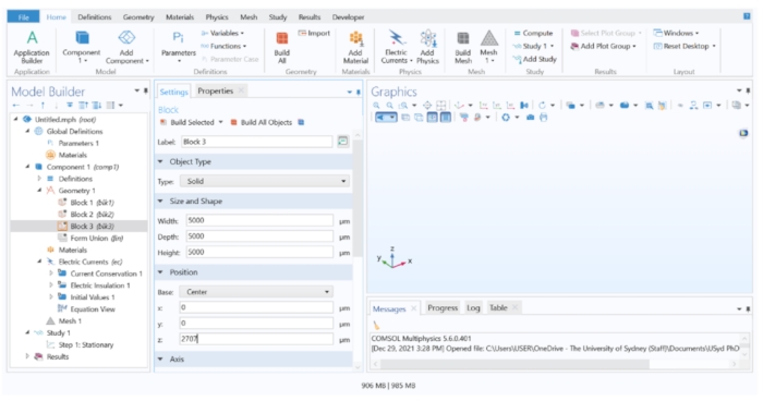
Figure 1: Creating the tisssue geometry. A block geometry was inserted into the FEM model to represent the tissue. Please click here to view a larger version of this figure.

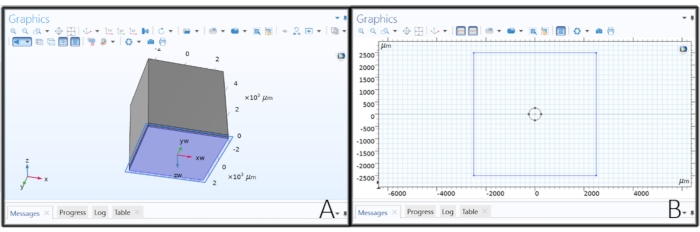
Figure 2: Creating the electrode's geometry. (A) Making a work plane to draw the disk electrode. (B) Sketching a circle on a work plane to create a disk electrode. Please click here to view a larger version of this figure.

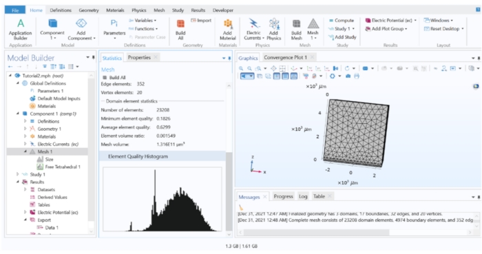
Figure 3: The element quality histogram of the FEM model. The histogram showed the quality of the elements throughout the model. Mesh refinements are needed if a significant portion of the elements are in the low quality region. Please click here to view a larger version of this figure.

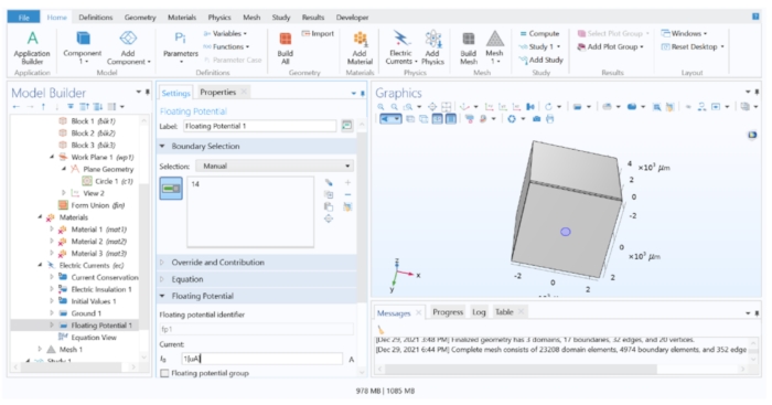
Figure 4: Assigning a current value to the electrode. A unitary current applied to the electrode's geometry in the FEM software. Please click here to view a larger version of this figure.

2. Importing the geometry of the neural cell in the neuron computational suite's GUI

1. Build the geometry of the cell model
   1. Importing the morphology using the Cell Builder feature.
      1. Run 'nrngui' from the neuron computational suite's installation folder, click on Tools > Miscellaneous > Import 3D, and then tick the Choose a File box.
      2. Locate the downloaded .swc file and click on Read. Once the geometry has been imported, click on Export > Cell Builder (Supplementary Figure 5).
   2. Creating a .hoc file of the imported cell morphology
      1. Go to the Subsets tab and observe the subsets that have been predefined in the model (e.g., soma, axon, basal, etc). Tick the Continuous Create box, go to Management > Export, and export the morphology as 'rgc.hoc'.
   3. Viewing the morphology of the cell
      1. Click on Tool > Model View > 1 Real Cells > Root Soma[0] on the toolbar, right-click on the appearing window and click on Axis Type > View Axis. By visual inspection, this model's dendritic field diameter is around 250 µm. Close the NEURON windows for now.

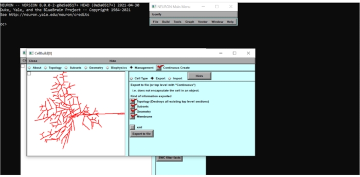
Figure 5: Exporting the neuron model information as a .hoc file. The geometry of the neuron was exported to a .hoc file to allow further modifications. Please click here to view a larger version of this figure.

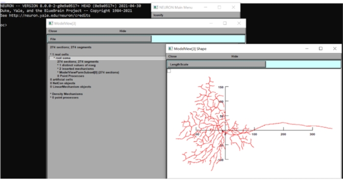
Figure 6: Measuring the dimension of the neuron. The morphology of the neuron (top view) was displayed in the GUI of the neuron computational suite with the x-y axes superimposed. The scale was in µm. Please click here to view a larger version of this figure.

3. Programming the NEURON computation simulation

1. Adjusting the cell's morphology by programming in .hoc language
   NOTE: The morphology of the cell can be adjusted via the GUI's Cell Builder feature. However, how this could be done by editing the .hoc file to speed up the process is demonstrated. The .hoc file defines the topology (physical connections between each part of the neurons), morphology (the length, diameter, and location of each neuron section) and the biophysical properties (ion channel parameters) of the modeled cell. The complete documentation for .hoc programming can be found in: https://neuron.yale.edu/neuron/static/new_doc/index.html#,
   1. Open the resulting .hoc file with a text editor (e.g., Notepad). Add an axon initial segment of 40 µm length and a narrow axonal segment of 90 µm length close to the soma as described in Sheasby and Fohlmeister¹⁷, as well as change the length of the dendrites so that the dendritic field size becomes 180 µm to match the G1 cell in Rockhill, et al.¹⁸.
      1. Creating new cell sections and defining the topological connections for each section.
         1. To create new cell sections for the axon initial segment (AIS) and the narrow axonal segment (NS), add these lines to the beginning of the rgc.hoc file:
            create AIS, NS // Declaring cell compartments called AIS and NS
            Then, replace the line 'connect axon(0), soma[1](1)' with:
            connect ais(0), soma[1](1) // Connecting the first segment of AIS to the end of soma[1]
            connect ns(0), ais(1) // Connecting the first segment of NS to the end of AIS
            connect axon(0), ns(1) // Connecting the first segment of the axon to the end of NS
      2. Defining the 3D positions, diameters, and length of the cell sections
         1. Define the 3D positions and diameters of the AIS and NS compartments by writing these lines inside the 'proc shape3d_31()' brackets:
            ais { pt3dadd(-2.25, -1.55, 0, 1) // The first three numbers are the xyz-coordinate, and the diameter is 1 µm
            pt3dadd(37.75, -1.55, 0, 1)} // The first point is at x = -2.25 µm and the last point is at x = 37.75 µm
            ns { pt3dadd(37.75, -1.55, 0, 0.3) // The 3D coordinates and the diameter for the NS segments
            pt3dadd(127.75, -1.55, 0, 0.3)}
         2. At the end of the file, shift the axon's 3D coordinate so that its initial point meets the end point of NS by typing:
            axon {for i=0,n3d()-1 {pt3dchange(i, x3d(i)+130, y3d(i),z3d(i)-5, diam3d(i))}} //Shift the x-coordinate
         3. At the end of the file, shorten the dendritic compartments by 18% by typing:
            forsec basal {L=L*0.82} // Scaling the length to make the dendritic field size smaller
            define_shape() // Filling in missing 3D information
2. Defining the number of segments for each section
   NOTE: Each section of the neuron can be spatially discretized, much like the process of meshing in the FEM model. The spatial discretization divides the neuron virtually into smaller segments where computations are to be done. For the number of segments 'nseg', make sure that odd numbers are used to ensure that there is an internal node at the midpoint of a cell section, and try tripling the nseg number until the computation produces a consistent result⁹. A higher number of segments will produce a more accurate numerical approximation but also increases the computational load.
   1. To exemplify the discretization process, add the following lines in the rgc.hoc file to divide the neuronal sections in the somatic and axonal subsets into several segments:
      forsec somatic {nseg=31}
      forsec axonal {nseg=301}
      Other sections in the model need to be discretized as well by typing these lines but changing the subset name (after 'forsec') and the number of segments (after 'nseg') as desired.
3. Insert customized ion channel mechanisms
   1. Writing customized ion channel mechanisms as .mod files: To apply the ion channel mechanisms, create .mod files and insert the files into the biophysical section part of the .hoc file by following steps 3.3.1-3.3.3. The .mod file contains the variables and the differential equations to be solved for each ion channel.
      NOTE: Correct ion channel mechanism definitions and implementations are critical in accurate neuron simulations. When writing .mod files, check whether the units are correct (the provided 'modlunit' utility that can be run to check unit consistency) and that the equations are written correctly. To test that the ion channel mechanisms are correct, the current for each ion channel during intracellular or extracellular stimulation can be plotted and compared to empirical findings.
      1. Voltage-gated ion channels
         NOTE: A .mod file to create a voltage-gated ion channel typically includes a DERIVATIVE block that has the differential equation to solve, a BREAKPOINT block that has the commands to solve the differential equations using a chosen numerical approximation method, and PROCEDURE blocks that tell the program to calculate the gating parameters (e.g., mt, ht, and d in this example). This code will calculate the values of the ionic current passing through the channel for each time step.
         1. To exemplify the process, create a voltage-dependent Ca channel that has first-order differential equations to solve for the gating variables.
         2. Open a new file in the text editor and type the lines in the Supplementary Material-Defining a voltage-dependent Cat channel. Save this file as Cat.mod in the same folder as the .hoc file. This process needs to be repeated for the other ion channels that the model neuron contains.
      2. Voltage- and concentration-dependent ion channels
         1. The kinetics of some ion channels, such as the calcium-activated potassium channels in the retinal ganglion cells, depend on the intracellular calcium concentration besides the transmembrane voltage¹⁹. To model this type of mechanism, create a file called KCa.mod, and type the lines as shown in Supplementary Material-Voltage- and concentration-dependent ion channels. In this .mod file, the variable 'cai', which is defined as the internal concentration of Ca ion was calculated, and then this variable is used in the equation to calculate the iKCa current.
   2. Compilation of .mod files
      1. Compile all the .mod files by running the neuron computational suite's mknrndll utility from the installation folder. Locate the folder where the .mod files are contained and click compile to create O and C files. After this, the mechanisms can be inserted into this cell model.
   3. Application of the .mod files in the main NEURON model file.
      NOTE: Besides inserting the ion channels, the maximum Na conductance was defined for the 'somatic' subset only. We could individually adjust the maximum membrane conductance for different neuronal segments if necessary.
      1. For brevity, combine all the ion channel mechanisms to a single .mod file (Supplementary Material-Complete .mod file). Insert the combined .mod file containing all the ion channels and a passive leak channel to all the segments in the 'somatic' subset by typing the lines below in the 'biophys' procedure of the rgc.hoc file:
         forsec somatic {insert rgcSpike
         insert pas // passive leak channel
         gnabar_rgcSpike = 80e-3
         g_pas = 0.008e-3 // leak membrane conductance}
   4. Setting the axoplasmic resistivity
      1. The cells have axoplasmic resistivity that can be changed per compartment. For this model, all segments have the same resistivity of 110 Ω·cm. Change the axoplasmic resistivity in the rgc.hoc file:
         forall {Ra = 110}
4. Insert extracellular mechanisms and define pulse waveform
   1. Inserting an extracellular mechanism into the cell model
      1. For the cell model to respond to extracellular voltage, insert an extracellular mechanism into all segments by typing the line at the bottom of the rgc.hoc file:
         forall {insert extracellular}
   2. Creating a biphasic pulse
      NOTE: In this demonstration, a constant current biphasic pulse is made that is user-adjustable in pulse width, interphase gap, and the number of repetitions by creating a procedure in a .hoc file. For a more structured program, use the rgc.hoc file as a file to create the cell model, while the stimulation process is applied in a separate .hoc file, which would load the cell model to which the stimulation is applied.
      1. Create a new text file called stimulation.hoc and start the code by loading the cell model file; then, make a biphasic pulse by defining a procedure as shown in Supplementary Material-Creating a biphasic pulse in the neuron simulation.
         NOTE: This step creates a constant current cathodic-first biphasic pulse where the stimulus parameters are to be declared by the user when running the simulation. Currently, the magnitude of the anodic and cathodic pulses is ±1 µA, but this magnitude needs to change depending on the stimulation current delivered by the disk electrode.

4. Running and automating multiple simulations

1. Combining the models
   1. Extracting the coordinates for the nodes in the neuron cell model
      NOTE: The purpose of combining the simulations is to acquire the extracellular potential values corresponding to each node of the cell model. The coordinates of the two models must, however, be aligned. In this example, the center segment of the soma (soma(0.5)) was aligned to lie on the horizontal midplane of the retinal tissue (corresponding to the retinal ganglion cell layer), with the center node of the soma located right above the center of the disk electrode.
      1. Open the FEM model, and note the coordinate of a reference point (e.g., the horizontal midplane of the retinal tissue, above the center of the disk electrode), in which case it is [0, 0, 131.5] µm.
      2. In the neuron computational suite, create a file called calculateCoord.hoc to extract the coordinates of each segment's centroid and shift each section so that the center segment of the soma has the same coordinate as the reference point in the FEM model (Supplementary Material-Calculating the coordinate of each node).
   2. Saving the coordinate points to a text file
      1. Run the calculateCoord.hoc file (either by double-clicking from the File Explorer or by opening GUI of the neuron computational suite; then, click on File > load hoc in the toolbar). Save the coordinates for the extracellular voltage values to be evaluated to a text file named 'coordinates.dat'.
   3. Running the simulations and saving the voltage data to a text file
      NOTE: In this step, we extracted the calculated extracellular values from the FEM model, but we would only save the data from the relevant coordinates that coincide with the centre of each cell segment. Follow step 4.1.6.2 when a large number of potentials are required to export.
      1. Open the tissue model file in the FEM software; go to the Results heading in the Model Tree, and click on Export > Data > Data 1. Make sure that the Dataset is set to Study 1/Parametric Solutions 1, and then type 'V' in the Expression column and 'mV' in the Unit column.
      2. Under Output, change the Filename to extracellular.dat, and choose Points to Evaluate in: From File. Load the coordinates.dat for the Coordinate File field, and then click on Export.
   4. Applying the biphasic pulse to the cell model
      NOTE: At this stage, the extracellular voltage values for each cell segment at one time point (where the current is 1 µA) is available. As the study intends to subject the cell to a biphasic pulse, make the extracellular voltage value experienced by the cell change with time using the 'vector.play' method.
      1. Add the lines shown in the Supplementary Material-Application of the biphasic pulse in the stimulation.hoc.
   5. Running the combined simulation
      NOTE: A time interval 'dt' for the numerical approximations needs to be defined to run the simulations. Similar to nseg, a shorter dt can increase the computational accuracy but also increases the computational cost.
      1. Add the lines shown in the Supplementary Material-Executing the neuron simulation to the end of the stimulation.hoc. Then, double-click on the stimulation.hoc file to load the script and automatically run the simulation. The transmembrane potential of the segment of interest can be displayed in the GUI of the neuron computational suite (step 4.2.1) or saved to a text file to be read in other programs (step 4.1.6.1.2). Follow steps 4.1.6.1 and 4.1.6.2 if repeated calculations and a large number of membrane potentials need to be exported.
   6. Extra: Automating simulations
      NOTE: To find a threshold amplitude, loop the simulation several times with a different current amplitude each time. Another automation might be needed to find the threshold for neurons located at different positions relative to the stimulating electrode. An automation step can be done in the neuron computational suite using a procedure, as well as in the FEM software using a script called a 'method'.
      1. Automation of neuron simulation to find a threshold amplitude
         NOTE: A batch of neuron simulations can be done automatically. The following steps are implemented in the neuron simulation program to find the threshold amplitudes of neurons under different stimulation parameters.
         1. Create a procedure to repeat simulation in the neuron simulation program: In the stimulation.hoc, create a vector to contain a range of current amplitude to test. Then, create a procedure to apply the current amplitude and record any presence of a spike (a positive change from a negative to a positive transmembrane voltage), and the threshold amplitude is defined as the lowest current amplitude that causes a spike to occur. To do this, define a procedure called findTh() (Supplementary Material-Looping over a range of current amplitudes) at the end of the stimulation.hoc file
         2. Saving the response at the threshold to a text file: Add the following lines to the findTh() procedure in the stimulation.hoc to store the calculated transmembrane voltage values for all neuron compartments from each time step in a text file:
            sprint(saveFileName, "Response_%d.dat", th) // Store the threshold value
            saveFile.wopen(saveFileName)
            for i=0,(responseVector.size()-1){
            saveFile.printf("%g, ", responseVector.x[i])
            if(i==responseVector.size()-1) {saveFile.printf("%g\n", responseVector.x[i])
            saveFile.close(saveFileName)
            }}
      2. Automation in the FEM software to find the voltage values for neurons in different locations
         NOTE: Another automation that can be done is the automatic acquisition of extracellular voltage values for neurons in different locations. The Application Builder menu in the FEM software provides a means to define a 'method', or a script to automate the steps needed for the software to perform calculations. To demonstrate, the location of the cell in the x-direction is shifted by 5 times in a 100 µm step (Supplementary Figure 6).
         1. Writing a code for automations of FEM simulations.
            1. Go to the Application Builder, right-click on Methods in the Application Builder tree, choose New Method, and click on OK. Go to File > Preferences > Methods, tick the View All Codes box, and click on OK.
            2. Write a .hoc script that will load the coordinate file, shift the values to match the desired location, and save a text file containing the voltage values for the new location of the cell by typing the codes shown in the Supplementary Material-Defining a method to automate FEM simulations.
         2. Running the automated steps in the FEM software: Switch to the Model Builder, Developer > Run Method > Method 1. This will produce .dat files with the appropriate voltage values, named extracellular_1.dat, extracellular_2.dat, etc.
      3. Looping the simulations in a general purpose programming language
         NOTE: To loop the simulations, the appropriate text file needs to be loaded to the neuron computational suite's simulation each time, and a programming language²⁰ that can load and manipulate text files easily is convenient to perform this step. Any convenient integrated development environment (IDE)²¹ can be used for this step.
         1. Open the chosen IDE, click on New File to make a new script. Here a .py file is used in this example. Type the lines shown in Supplementary Material-Running the simulations in a general purpose programming language.
         2. Finally, click on Run or press F5 to run the script, which will also open the GUI (Supplementary Figure 7).
2. Display of simulation data
   NOTE: By following all the steps above, the simulation results should be stored in text files, containing the threshold value and the transmembrane potential at the threshold. However, the user has the option to display the simulation result while the simulation is running using NEURON's GUI.
   1. Graph the response of the neuron model to the extracellular stimulation in the neuron computational suite's GUI. To do this, run stimulation.hoc, click on Graph > Voltage Axis from the toolbar, and on the graph window, right-click anywhere and choose Plot What.
   2. Type in 'axon.v(1)' in the Variable to Graph field, which means that it will plot the transmembrane potential of the last segment of the axon per time step.

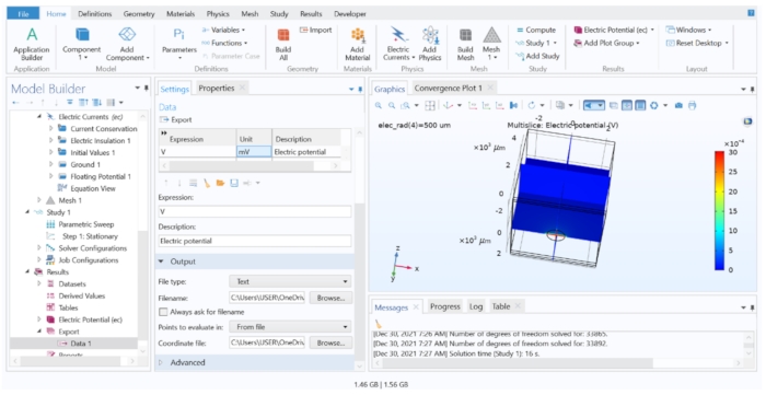
Figure 7: Displaying and exporting the FEM computation results to a text file. The Graphics window showing a Multislice plot of the electric potential in V. The options in the Data Export Setting allowed exporting the calculated variable into a text file. Please click here to view a larger version of this figure.

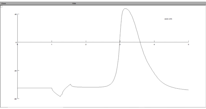
Figure 8: Displaying the graph of the transmembrane potential using a voltage graph. The neuron transmembrane potential was displayed in the GUI of the neuron computational suite. The x-axis is time in ms, while the y-axis is the transmembrane potential of the chosen neuron segment in mV. Please click here to view a larger version of this figure.

Results

We conducted two simulation protocols to demonstrate the use of the model. The first protocol involved varying the electrode size while keeping the location of the neuron and the electrical pulse parameters the same. The second protocol involved shifting the neuron in the x-direction in 100 µm steps, while the size of the electrode remained constant. For both protocols, the pulse used was a single cathodic-first biphasic pulse of 0.25 ms width with a 0.05 ms interphase gap. For the first protocol, the radius of the elect...

Discussion

In this paper, we have demonstrated a modeling workflow that combined finite element and biophysical neuron modeling. The model is highly flexible, as it can be modified in its complexity to fit different purposes, and it provides a way to validate the results against empirical findings. We also demonstrated how we parameterized the model to enable automation.

The two-step modeling method combines the advantages of using FEM and neuron computational suite to solve the neuron's cable equation i...

Materials

List of materials used in this article

Name	Company	Catalog Number	Comments
Computer workstation	N/A	N/A	Windows 64-bit operating system, at least 4GB of RAM, at least 3 GB of disk space
Anaconda Python	Anaconda Inc.	Version 3.9	The open source Individual Edition containing Python 3.9 and preinstalled packages to perform data manipulation, as well as Spyder Integrated Development Environment. It could be used to control the simulation, as well as to display and analyse the simulation data.
COMSOL Multiphysics	COMSOL	Version 5.6	The simulation suite to perform finite element modelling. The licence for the AC/DC module should be purchased. The Application Builder capability should be included in the licence to follow the automation tutorial.
NEURON	NEURON	Version 8.0	A freely-distributed software to perform the computation of neuronal cells and/or neural networks.

References

- Greenberg, R. J., Velte, T. J., Humayun, M. S., Scarlatis, G. N., de Juan, E. A computational model of electrical stimulation of the retinal ganglion cell. IEEE Transactions on Bio-medical Engineering. 46 (5), 505-514 (1999).
- Guo, T., et al. Mediating retinal ganglion cell spike rates using high-frequency electrical stimulation. Frontiers in Neuroscience. 13, 413(2019).
- Loizos, K., et al. Increasing electrical stimulation efficacy in degenerated retina: Stimulus waveform design in a multiscale computational model. IEEE Transactions on Neural Systems and Rehabilitation Engineering. 26 (6), 1111-1120 (2018).
- Cao, X., Sui, X., Lyu, Q., Li, L., Chai, X. Effects of different three-dimensional electrodes on epiretinal electrical stimulation by modeling analysis. Journal of Neuroengineering and Rehabilitation. 12 (1), 73(2015).
- Wilke, R. G. H., Moghadam, G. K., Lovell, N. H., Suaning, G. J., Dokos, S. Electric crosstalk impairs spatial resolution of multi-electrode arrays in retinal implants. Journal of Neural Engineering. 8 (4), 046016(2011).
- AC/DC module user's guide. COMSOL AB. , Available from: https://doc.comsol.com/5.4/doc/com.comsol.help.acdc/ACDCModuleUsersGuide.pdf (2018).
- Malmivuo, P., Malmivuo, J., Plonsey, R. Bioelectromagnetism: Principles and Applications of Bioelectric and Biomagnetic Fields. , Oxford University Press. New York. (1995).
- Rall, W. Electrophysiology of a dendritic neuron model. Biophysical Journal. 2, 145-167 (1962).
- Carnevale, N. T., Hines, M. L. The Neuron Book. , Cambridge University Press. Cambridge. (2006).
- Rattay, F. The basic mechanism for the electrical stimulation of the nervous system. Neuroscience. 89 (2), 335-346 (1999).
- Hodgkin, A. L., Huxley, A. F. A quantitative description of membrane current and its application to conduction and excitation in nerve. The Journal of Physiology. 117 (4), 500-544 (1952).
- Liang, T., et al. Threshold suprachoroidal-transretinal stimulation current required by different-size electrodes in rabbit eyes. Ophthalmic Research. 45 (3), 113-121 (2011).
- Jensen, R. J., Rizzo, J. F., Ziv, O. R., Grumet, A., Wyatt, J. Thresholds for activation of rabbit retinal ganglion cells with an ultrafine, extracellular microelectrode. Investigative Ophthalmology and Visual Science. 44 (8), 3533-3543 (2003).
- Kim, W., Choi, M., Kim, S. -W. The normative retinal and choroidal thicknesses of the rabbit as revealed by spectral domain optical coherence tomography. Journal of the Korean Ophthalmological Society. 62 (3), 354-361 (2021).
- Guo, T., et al. Influence of cell morphology in a computational model of ON and OFF retinal ganglion cells. 35th Annual International Conference of the IEEE Engineering in Medicine and Biology Society (EMBC). 2013, 4553-4556 (2013).
- Haberbosch, L., et al. Safety aspects, tolerability and modeling of retinofugal alternating current stimulation. Frontiers in Neuroscience. 13, 783(2019).
- Sheasby, B. W., Fohlmeister, J. F. Impulse encoding across the dendritic morphologies of retinal ganglion cells. Journal of Neurophysiology. 81 (4), 1685-1698 (1999).
- Rockhill, R. L., Daly, F. J., MacNeil, M. A., Brown, S. P., Masland, R. H. The diversity of ganglion cells in a mammalian retina. Journal of Neuroscience. 22 (9), 3831-3843 (2002).
- Lukasiewicz, P., Werblin, F. A slowly inactivating potassium current truncates spike activity in ganglion cells of the tiger salamander retina. The Journal of Neuroscience: The Official Journal of the Society for Neuroscience. 8 (12), 4470-4481 (1988).
- Van Rossum, G. Python Reference Manual. , CWI: Centrum voor Wiskunde en Informatica. Amsterdam. (1995).
- Spyder Doc Contributors. Welcome to Spyder's Documentation - Spyder 5 documentation. , Available from: https://docs.spyder-idle.org/current/index.html (2022).
- Rattay, F. Ways to approximate current-distance relations for electrically stimulated fibers. Journal of Theoretical Biology. 125 (3), 339-349 (1987).
- Tsai, D., Morley, J. W., Suaning, G. J., Lovell, N. H. Direct activation and temporal response properties of rabbit retinal ganglion cells following subretinal stimulation. Journal of Neurophysiology. 102 (5), 2982-2993 (2009).
- Tsai, D., Morley, J. W., Suaning, G. J., Lovell, N. H. Frequency-dependent reduction of voltage-gated sodium current modulates retinal ganglion cell response rate to electrical stimulation. Journal of Neural Engineering. 8 (6), 066007(2011).
- Joucla, S., Glière, A., Yvert, B. Current approaches to model extracellular electrical neural microstimulation. Frontiers in Computational Neuroscience. 8, 13(2014).
- OpenFOAM. , Available from: https://www.openfoam.com/ (2022).
- Barba, L., Forsyth, G. CFD Python: The 12 steps to Navier-Stokes equations. Journal of Open Source Education. 1 (9), 21(2018).
Access restricted. Please log in or start a trial to view this content.
Reprints and Permissions