Using the MouseWalker to Quantify Locomotor Dysfunction in a Mouse Model of Spinal Cord Injury

Summary

An experimental pipeline to quantitatively describe the locomotor pattern of freely walking mice using the MouseWalker (MW) toolbox is provided, ranging from initial video recordings and tracking to post-quantification analysis. A spinal cord contusion injury model in mice is employed to demonstrate the usefulness of the MW system.

Abstract

The execution of complex and highly coordinated motor programs, such as walking and running, is dependent on the rhythmic activation of spinal and supra-spinal circuits. After a thoracic spinal cord injury, communication with upstream circuits is impaired. This, in turn, leads to a loss of coordination, with limited recovery potential. Hence, to better evaluate the degree of recovery after the administration of drugs or therapies, there is a necessity for new, more detailed, and accurate tools to quantify gait, limb coordination, and other fine aspects of locomotor behavior in animal models of spinal cord injury. Several assays have been developed over the years to quantitatively assess free-walking behavior in rodents; however, they usually lack direct measurements related to stepping gait strategies, footprint patterns, and coordination. To address these shortcomings, an updated version of the MouseWalker, which combines a frustrated total internal reflection (fTIR) walkway with tracking and quantification software, is provided. This open-source system has been adapted to extract several graphical outputs and kinematic parameters, and a set of post-quantification tools can be to analyze the output data provided. This manuscript also demonstrates how this method, allied with already established behavioral tests, quantitatively describes locomotor deficits following spinal cord injury.

Introduction

The effective coordination of four limbs is not unique to quadruped animals. Forelimb-hindlimb coordination in humans remains important to accomplish several tasks, such as swimming and alterations of speed while walking¹. Various limb kinematic² and motor program^1,3,4, as well as proprioceptive feedback circuits⁵, are conserved between humans and other mammals and should be considered when analyzing therapeutic options for motor disorders, such as spinal cord injury (SCI)^6,7,8.

In order to walk, several spinal connections from the forelimbs and hindlimbs need to be properly wired and rhythmically activated, which requires inputs from the brain and feedback from the somatosensory system^2,9,10. These connections culminate in the central pattern generators (CPGs), which are situated at a cervical and lumbar level for the forelimbs and hindlimbs, respectively^1,9,10. Often, after SCI, the disruption of neuronal connectivity and the formation of an inhibitory glial scar¹² limit the recovery of locomotor function, with outcomes varying from total paralysis to restricted function of a group of limbs depending on the injury severity. Tools to precisely quantify locomotor function after SCI are critical for monitoring recovery and evaluating the effects of treatments or other clinical interventions⁶.

The standard metric assay for mouse contusion models of SCI is the Basso mouse scale (BMS)^13,14, a non-parametric score that considers trunk stability, tail position, plantar stepping, and forelimb-hindlimb coordination in an open field arena. Even though the BMS is extremely reliable for most cases, it requires at least two experienced raters to observe all the angles of animal movement in order to account for natural variability and reduce bias.

Other assays have also been developed to assess motor performance after SCI quantitatively. These include the rotarod test, which measures time spent on a rotating cylinder¹⁵; the horizontal ladder, which measures the number of missed railings and positive ladder grabs^16,17; and the beam walking test, which measures the time an animal takes and the number of failures it makes when crossing a narrow beam¹⁸. Despite reflecting a combination of motor deficits, none of these tests produce direct locomotor information about forelimb-hindlimb coordination.

To specifically and more thoroughly analyze walking behavior, other assays have been developed to reconstruct step cycles and gaiting strategies. One example is the footprint test, where the inked paws of an animal draw a pattern over a sheet of white paper¹⁹. Although simple in its execution, extracting kinematic parameters such as stride length is cumbersome and inaccurate. Moreover, the lack of dynamic parameters, such as the duration of the step cycle or leg-timed coordination, limits its applications; indeed, these dynamic parameters can only be acquired by analyzing frame-by-frame videos of rodents walking through a transparent surface. For SCI studies, researchers have analyzed walking behavior from a lateral view using a treadmill, including reconstructing the step cycle and measuring the angular variations of each leg joint^4,20,21. Even though this approach can be extremely informative⁶, it remains focused on a specific set of limbs and lacks additional gait features, such as coordination.

To fill these gaps, Hamers and colleagues developed a quantitative test based on an optical touch sensor using frustrated total internal reflection (fTIR)²². In this method, light propagates through glass via internal reflection, becomes scattered upon paw pressing, and, finally, is captured by a high-speed camera. More recently, an open-source version of this method, called MouseWalker, was made available, and this approach combines an fTIR walkway with a tracking and quantification software package²³. Using this method, the user can extract a large set of quantitative parameters, including step, spatial, and gait patterns, footprint positioning, and forelimb-hindlimb coordination, as well as visual outputs, such as footprint patterns (mimicking the inked paw assay⁶) or stance phases relative to the body axis. Importantly, due to its open-source nature, new parameters can be extracted by updating the MATLAB script package.

Here, the previously published assembly of the MouseWalker²³ system is updated. A description of how to set it up is provided, with all the steps required to achieve the best video quality, tracking conditions, and parameter acquisition. Additional post-quantification tools are also shared to enhance the analysis of the MouseWalker (MW) output dataset. Finally, the usefulness of this tool is demonstrated by obtaining quantifiable values for general locomotor performance, specifically step cycles and forelimb-hindlimb coordination, in a spinal cord injury (SCI) context.

Protocol

All handling, surgical, and post-operative care procedures were approved by Instituto de Medicina Molecular Internal Committee (ORBEA) and the Portuguese Animal Ethics Committee (DGAV) in accordance with the European Community guidelines (Directive 2010/63/EU) and the Portuguese law on animal care (DL 113/2013) under the license 0421/000/000/2022. Female C57Bl/6J mice aged 9 weeks were used for the present study. All efforts were made to minimize the number of animals and to decrease the suffering of the animals used in the study. The MATLAB script and the standalone version of the MW software are open-source and are available at the GitHub
repository (https://github.com/NeurogeneLocomotion/MouseWalker). While the MW software was developed in MATLAB R2012b, it has been adapted to run in MATLAB R2022b. Figure 1 illustrates the analysis workflow of the MW.

1. Setting up the MouseWalker (MW) apparatus

1. Assemble the MW apparatus as described previously²³, or adapt to the specific needs of the experimental design (see Table of Materials and Supplementary Figure 1 for more details on the setup).
   NOTE: The walking arena can be made wider to accommodate larger animals, such as rats.
2. Verify that the plexiglass where the animals walk is clean and scratch-free. Use a smooth cleaning cloth, and minimize the use of organic solvents such as ammonia or ethanol in high concentrations, which can damage the plexiglass (3% hydrogen peroxide, 7% ethanol, or any compatible and appropriate disinfectant for plexiglass is recommended). If necessary, replace the plexiglass.
3. Set up the high-speed camera with a fast lens and a large aperture (i.e., smaller F-stop values) to capture a large amount of light, as this helps to record the fTIR signals (see Table of Materials).
   NOTE: The lens should not generate optical distortions, particularly at the edges of the image. Optical distortions can be tested by recording a known pattern (e.g., stripes or squares) and then measuring the size of the blocks on ImageJ/FIJI²⁴ (use the line tool, and then click on Analyze > Measure). For example, a 1 cm sized square should have the same pixel dimensions both at the center of the image and on the edges. Variations should be smaller than 5%.
4. Light up the multicolored LED light strip from the background light box.
5. Light up the white LED light strip from the walkway light box.
   NOTE: A colored LED can also be used²⁵ to facilitate the distinction of the footprint/body/background.
6. With the room lights off, verify the light intensity of the background light box and walkway. Adjust the intensity, if necessary, using a potentiometer or semi-opaque plastic. These must be optimized so that pixel intensity increases in the following order: animal's body < background < footprints.
   1. To check the pixel intensity of the animal's body/background/footprints, open the image sequence on ImageJ/FIJI²⁴, and click on Analyze > Measure. The footprint signal should not be oversaturated, as this will prevent the boundaries of the footprint from being defined (i.e., toes and foot pads) (Supplementary Figure 2).
7. Adjust the image contrast of the walkway on the video recording software. The contrast can be adjusted in two ways: by dimming or increasing the lighting on the LED strip or by adjusting the camera lens aperture.
8. Position the lens correctly to be at the same height and in the center of the 45° reflecting mirror and perpendicular (90°) to the walkway. This will generate a constantly proportional image along the left-right walkway.
   NOTE: Avoid changing the camera position (distance, height, and orientation) across the multiple recording sessions. If necessary, mark the floor where the tripod should be placed. This will maintain the image features.
9. Focus the lens on the surface of the plexiglass. This can be tested using a non-damaging object touching the surface of the plexiglass.
   ​NOTE: With lower F-stop lens values, the depth of field will become smaller, thus making focusing harder.
10. Ensure all the settings remain unaltered during the assay, as they may change the pixel intensity of the recorded videos.

2. Video acquisition

1. Ensure the mice are familiar with the room and apparatus prior to testing. Save at least 1 day for habituation (day 0). To avoid excessive training, perform the MW test on a different day from the other behavioral tests (preferably the day after).
2. In the video recording software, ensure at least 50 cm of the walkway is visible.
3. Adjust the recording settings to truncate the walkway region. This will reduce the video size and optimize the video acquisition.
4. Take a picture or a short video of a regular ruler before each session. The number of pixels per centimeter will later be used in the "settings window" to calibrate the videos.
5. Start the video acquisition, and place the animal on the edge of the walkway by grasping the base of the tail to avoid injuries. Ensure the animals move forward to the extreme edge of the platform. Perform the video recordings with at least 100 frames/s to ensure smooth gait transitions.
   1. If needed, motivate the animals to move by gently tapping the walkway wall or snapping/clapping the fingers. However, avoid physical nudging, as this may affect the results.
   2. Save the videos directly as image sequences in TIFF (with LZW compression), JPEG, or PNG format. In case the camera records as a raw MOV file, convert the videos into image sequences by opening the file in ImageJ/FIJI²⁴ and clicking on File > Save as > Image sequence (or by using other software, such as LosslessCut²⁵).
      ​NOTE: Most animals start walking immediately after being put in the walkway; therefore, it is recommended to start the video acquisition before placing the animal.

3. Preparing the videos for the MW tracking software

1. Film enough complete runs of each individual mouse. The number of animals to film per condition and the number of complete runs must be decided according to each experimental design. A complete run is when the mouse walks the complete 50 cm of the walkway without prolonged stops (in this experiment, three complete runs were selected).
   NOTE: Depending on the image acquisition software, videos may need to be cropped to the smallest ROI. This will increase the speed of tracking and output generation.
2. In ImageJ/FIJI²⁴, select the frames in which the mouse is on the screen by clicking on Image > Stack > Tools > Make a substack. The tracking on the MW requires the head and the tail to be visible in all the frames. It is possible, however, to make several substacks from a single video recording, which will later represent each run.
3. Save each substack separately in different folders by clicking on File > Save as > Image sequence. The MW software later creates a subfolder automatically in each directory every time one starts analyzing a run.

4. Tracking

1. Open MATLAB, add the folder containing the MW script to the working directory, and run "MouseWalker.m" on the main command line.
   NOTE: Using the MW software under MATLAB allows tracking error messages to be viewed on MATLAB's main console and the desired output data to be selected (by opening the main script file "MouseEvaluate.m" and changing the outputs to either 1 or 0: the excel file, footstep plots, stance traces, and gait patterns).
2. Load the video folder as the "Input directory". One can also choose the output folder; however, this is not a requirement as the MW software creates a new folder called "Results" automatically inside the "Input directory".
3. Using the arrows "<<", "<", ">>", and ">" check if the video frames are all loaded correctly inside the MW software.
4. Go to the "Settings window" where all the calibration and threshold parameters are located. These settings can change depending on the pixel intensity of the background and footprints, as well as the minimal size of the body and footprints, amongst other factors (see example in Supplementary Figure 2). Test the effect of changing some parameters by clicking on the Preview button.
   1. Use the different plot styles, including "body + feet + tail", "body only", "feet only", and "tail only", to help discriminate body parts after adjusting the threshold parameters.
   2. Take advantage of the tools on the right-side panel to take measurements of the brightness or size (using the "brightness" and "ruler" buttons, respectively). All settings can be saved as "default" as long as the camera distance remains the same.
5. After adjusting the threshold parameters, check that the video is ready for automated tracking. Go to the first frame, and click on Auto to start tracking. This step can be followed in real time, and it takes a few minutes, depending on the size of the video and the computer's performance.
   1. If the auto-tracking incorrectly labels the body features, cancel the auto-tracking, enter new settings, and restart the process.
6. After the tracking is completed, check if a manual correction is needed. To correct, use the middle panel to select or deselect, and indicate the location of the right fore (RF), right hind (RH), left fore (LF), and left hind (LH) paw footprints, head, nose, body (divided into two segments), and tail positions (divided into four segments). Save the changes by pressing the Save button.
   NOTE: All buttons and most commands have a key shortcut (check the associated manual for details²³). To facilitate video scrolling and the execution of keyboard shortcuts, a hardware controller with programmable buttons and a shuttle wheel like the Contour ShuttlePro V2 can be used.
7. Click on Evaluate to generate the output files from the tracked video. Depending on the desired output selected (see step 4.1), this step can take a few minutes.
8. Check that all the graphical output data plots are saved in the "Results" folder. Verify the accuracy of the tracking by examining some of the graphical outputs, such as the "Stance traces", where one can check if all the paw positions are consistent.
   1. If an error is identified, manually correct the tracking (if possible; otherwise, eliminate the "Results" folder, and perform the auto-tracking again with new settings), and click on the Evaluate command again.
9. Check that all the quantitative measurements generated by the MW software are saved on an Excel spreadsheet and summarized on "1. Info_Sheet". Ensure that the excel options for the formula delimitations match the script. The decimal separator must be ",", and the thousand separators must be ";".
10. Use the "MouseMultiEvaluate.m" script to congregate the measurements from all the runs into a new file for analysis.
    1. To begin, generate a .txt file containing the folder paths for all the videos (e.g. "Videofiles.txt"). Ensure that each line corresponds to a single video.
    2. Then, write "MouseMultiEvaluate('Videofiles.txt')" into the command line. An excel file named "ResultSummary.xls" will be generated in the working directory (see an example in the GitHub repository).
       ​NOTE: Figure 2 represents the graphical outputs obtained by the MW software from the videos of one recorded animal.

5. Kinematic data analysis workflow

1. Edit the excel sheet generated in step 4.10, which contains the data for processing using the supplied Python scripts, according to the following prerequisites.
   1. In the first column header, specify the experimental condition. Name each line following the group/condition name (individuals from the same groups must have the same name). The first group must be the control or baseline (this is only mandatory for heatmap plotting, step 5.6).
   2. In the second column, specify the animal ID. This is mandatory, although this information will not be used for plot generation.
   3. In the third column onward, choose the motor parameters that will be used for the analysis. Ensure that the first line is the name of the parameter (these names will later appear in the plots).
2. Open Anaconda Navigator, and execute Spyder to open the supplied Python scripts.
   NOTE: All the scripts were developed with Python 3.9.13, were executed with Spyder 5.2.2 in Anaconda Navigator 2.1.4, and are available in the Table of Materials and the GitHub repository (where additional materials are included, such as a video example, an excel example file, and an FAQs document). It is possible to execute the scripts outside the Anaconda Navigator; however, this graphical user interface is more user-friendly.
3. Use the "Rawdata_PlotGenerator.py" to generate the raw data plots. This will allow the visualization of each parameter as a function of speed.
   1. Open "Rawdata_PlotGenerator.py" in Spyder, and run the code by clicking on the Play button.
   2. Select the Excel file to analyze and the sheet name in the automatic window. If the sheet name was not altered, write "Sheet1".
   3. The raw data plots will appear in the plot console (upper right panel). To save the plots, click on the Save image or Save all images button in the plot console.
4. Use the script "Residuals_DataAnalysis" to calculate the residuals for data analysis. This script will generate a CSV file with the calculations of the residuals for all the motor parameters.
   NOTE: Many of the measured gait parameters extracted by the MW vary with speed (e.g., swing speed, step length, stance duration, stance straightness, and gait indexes). Therefore, it is recommended to perform a best-fit regression model of each individual parameter versus speed for the baseline experiment and to then determine the residual values for each experimental group in relation to this regression model. The data are then expressed as the difference from the residual normalized line²⁶.
   1. Open "Residuals_DataAnalysis.py" in Spyder, and run the code by clicking on the Play button.
   2. Select the Excel file to analyze and the sheet name in the automatic window. If the sheet name was not altered, write "Sheet1".
   3. Save the CSV file in the same folder as the data. It is mandatory that the control (or baseline) is the first group in the Excel file.
5. Use the "PCA_PlotGenerator.py" script to perform a principal component analysis (PCA).
   NOTE: This unsupervised dimensionality reduction method is used to generate a more succinct representation^27,28,29 of the data (Figure 3A, B). The PCA script includes the following steps. The data is first pre-processed by centering and scaling, after which the PCA algorithm computes the covariance matrix to determine the correlations between the variables and calculate the eigenvectors and eigenvalues of the covariance matrix to identify the principal components. The first two or three principal components are chosen for the representation of the data in 2D or 3D plots, respectively. Each dot in the plots corresponds to an animal and represents a different abstract variable. Color-coded dots are used to distinguish the specific groups. As such, clusters of dots reflect similar walking patterns shared by the corresponding individuals.
   1. Open "PCA_PlotGenerator.py" in Spyder, and run the code by clicking on the Play button.
   2. Select the Excel file to analyze and the sheet name in the automatic window. If the sheet name was not altered, write "Sheet1".
   3. Ensure that the PCA 2D and 3D plots appear in the plot console (upper-right panel). Each color represents a different group, and the legend appears next to the plot. To save the plot, click on Save image in the plot console.
6. Use "Heatmap_PlotGenerator.py" to generate a heatmap. Ensure that the heatmap generator creates a table showing the statistical differences between the baseline group (or control group) and the other groups for each motor parameter²⁷ (Figure 4). Each column depicts one group, and each line relates to a specific motor parameter.
   NOTE: Statistical analysis was conducted with a one-way ANOVA followed by Tukey's post hoc test (for normal distributions) or a Kruskal-Wallis ANOVA followed by Dunn's post hoc test (for non-normal distributions). Outliers were excluded from the analysis. P-values are represented by a color code, with red and blue shades indicating an increase or decrease relative to control (or baseline), respectively. The color shade represents the statistical significance, with darker colors showing a higher significance, and lighter colors showing a lower significance. *** corresponds to P < 0.001; ** corresponds to P < 0.01; and * corresponds to P < 0.05. White indicates no variation.
   1. Open "Heatmap_PlotGenerator.py" in Spyder, and run the code by clicking on the Play button.
   2. Select the Excel file to analyze and the sheet name in the automatic window. If the sheet name was not altered, write "Sheet1".
   3. Select the type of data in the second automatic window: raw data or residuals data. If an option is not selected, residuals data is the default.
   4. The heatmap will appear in the plot console (upper-right panel). To save the plot, click on Save image in the plot console.
      NOTE: It is mandatory that the control (or baseline) is the first group in the Excel file.
7. Use "Boxplots_PlotGenerator.py" to generate the boxplots. This tool will allow the generation of boxplots that represent the distribution of values for all the motor parameters for each group (Figure 5, Figure 6, and Figure 7).
   NOTE: Each box contains the median as the middle line, and the lower and upper edges of the boxes represent the 25% and 75% quartiles, respectively. The whiskers represent the range of the full data set, excluding outliers. Outliers are defined as any value that is 1.5 times the interquartile range below or above the 25% and 75% quartiles, respectively.
   1. Open "Boxplots_PlotGenerator.py" in Spyder, and run the code by clicking on the Play button.
   2. Select the Excel file to analyze and the sheet name in the automatic window. If the sheet name was not altered, write "Sheet1".
   3. Select the type of data in the second automatic window: raw data or residuals data. If an option is not selected, residuals data is the default.
   4. The boxplots will appear in the plot console (upper-right panel). To save the plots, click on the Save image or Save all images button in the plot console.

Results

The standard BMS system describes the gross motor deficits after SCI¹⁴. Due to its subjective nature, other quantitative assays are generally performed alongside the BMS to produce a more detailed and fine assessment of locomotion. However, these tests fail to show specific information about step cycles, stepping patterns, and forelimb-hindlimb coordination, which is extremely important in understanding how the spinal circuitry maintains function and adapts to an incomplete SCI. This section shows how the MW toolbox can help monitor the recovery of locomotor function after SCI and add relevant information about walking behavior.

The study sample was divided into two groups of female C57Bl/6J mice aged 9 weeks old: an SCI experimental group (n = 11), in which the animals underwent laminectomy followed by a moderate to severe contusion injury at the level of the T9/T10 vertebral column using an Infinite Horizon Impactor (see Table of Materials); and a sham-injured control group (n = 10), in which only the laminectomy was performed at the same column level (Figure 1, step 1). The locomotor behavior of the SCI and sham-injured animals was monitored for 30 days. The MW test was performed on the habituation day before the surgery (baseline) and 15 days, 22 days, and 30 days post-injury (dpi) (Figure 1, step 2). For the sake of comparison, the mice were subjected to the BMS test in parallel before the surgery and at 1 dpi, 3 dpi, 7 dpi, 14 dpi, 21 dpi, and 30 dpi (Supplementary Figure 3). After tracking all the videos obtained with the MW, two types of output files were then generated: graphical outputs, showing visual representations of several parameters after each run, and kinematic outputs, summarizing all the measurable motor parameters (Figure 1, step 3 and step 4).

Consequently, using a set of Python scripts (see Table of Materials and the GitHub repository link), the raw data plots were obtained (Figure 1, step 5). As most parameters are influenced by the speed of the animal, a regression model of the baseline group before the injury was performed together with the measured residual values for each condition (Figure 1, step 6). To check for kinematic profiles and significant differences between the control (sham) and experimental groups (SCI), all the kinematic parameters (total of 79) were subjected to a three-order principal component analysis (PCA), and a heatmap was generated with a collection of motor parameters that best described the dataset (total of 33) (Figure 1, step 7a,b). Finally, specific motor parameters that were affected after the SCI were compared to the baseline before the injury (Figure 1, Step 7c).

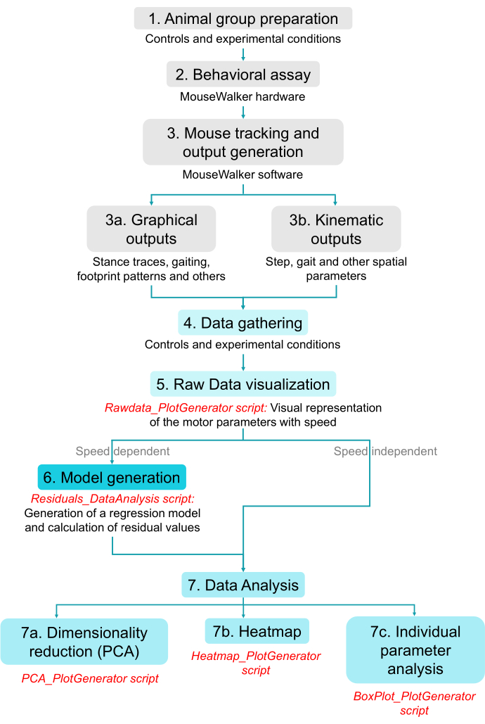
Figure 1: Schematic representation of the analysis workflow of the MW. (1) The animals are selected for laminectomy (sham control group) or laminectomy followed by a spinal cord injury (experimental group). (2) The animals are then subjected to a behavioral assay the day before the injury and on days 15, 22, and 30 post-injury. (3) The MW generates two types of output data: (a) graphical visualizations of several parameters, such as stance traces, gaiting, and stepping patterns, and (b) a kinematic summary of all the measurable motor parameters. (4) All the control and experimental data are congregated into a single file using the "MouseMultiEvaluate.m" script on MATLAB. (5) The "RawData_PlotGenerator" script for Python generates a visual representation of how all the measurable motor parameters vary according to speed. If the parameters do not correlate with speed, one could skip to (7); however, as most parameters after SCI strongly depend on speed, a model should be generated (6) using the "Residual_DataAnalysis" script for Python. After generating the residual values for each motor parameter, data analysis is carried out (7): (a) a principal component analysis (PCA) is performed using a selection of parameters with a "PCA_PlotGenerator" script; (b) a heatmap is created with a "Heatmap_PlotGenerator" script, to show the statistically significant differences between conditions for different parameters; and c) several individual parameters that are altered after SCI are evaluated with the "BoxPlot_PlotGenerator" script. All scripts are available in Table of Materials and GitHub repository link. The scripts are shown in red. Please click here to view a larger version of this figure.

From the graphical output data gathered from the MW, it was possible to confirm the well-known abrupt change in the visual display of the footprints after SCI. In the "Digital-ink" assay generated by the MW, lack of support of the hindpaws was detected (Figure 2A), together with a decrease in the footprint area for both the left and right hindpaws (Figure 2B), which was maintained from 15 dpi onward (data not shown). In addition, within each step cycle, the MW computes parameters related to the stance phase (i.e., the time between the paw touchdown and before lift-off) and the swing phase (i.e., the time the limb is off the ground). As such, the MW can generate visual "stance traces", which take into consideration the position of the body's center and axis in relation to each leg and their footprint center during the stance phases²³. The overall stance traces obtained for each animal displayed several unique features (Figure 2C). This data showed that after SCI, the hindpaws had shorter stance traces and more random paw positioning at both touchdown and lift-off from 15 dpi onward (Figure 2C).

Figure 2: Representative graphical outputs obtained by the MW software from the tracking videos. (A) "Digital-ink" prints for one SCI animal showing each paw with a different color: red (right fore), yellow (left fore), green (right hind), and blue (left hind) at several time points. (B) Footprints for the left fore (LF), left hind (LH), right fore (RF), and right hind (RH) of one SCI animal at 15 dpi. (C) "Stance traces" for one SCI animal at several time points. The AEP and PEP for one of the legs are illustrated in the first panel. The "footprint clustering" for both the AEP and PEP corresponds to the standard deviation of the average AEP or PEP coordinates in each video. Abbreviations: dpi = days post-injury; cm = centimeter; px = pixel. Please click here to view a larger version of this figure.

Next, the kinematic outputs were analyzed after being computed by the MW (Figure 3 and Figure 4). To obtain a more concise depiction of the dataset and test whether the kinematic motor parameters obtained from the MW were enough to depict locomotor deficits found in SCI animals across time, a PCA²⁷ was performed. Noticeably, 40% of the variance in the data could be explained in the first component (PC1: 40.1%), which segregated the group of animals that had an SCI from the rest, with a p-value lower than 0.001 based on a one-way ANOVA test (Figure 3A,B) at all time points (15 dpi, 22 dpi, and 30 dpi). There was also a poor contribution from the other components (PC2: 11% and PC3:8.6%). The assigned weight of each motor parameter contribution for each component is illustrated in Supplementary Figure 4. Moreover, the variance in the dataset was not enough to reflect differences across time (i.e., between 15 dpi, 22 dpi, and 30 dpi), which replicates the previously described plateau of locomotor recovery¹⁴. Altogether, these results indicate that the kinematic parameters obtained from the MW strongly describe the motor deficits observed after SCI across all time points.

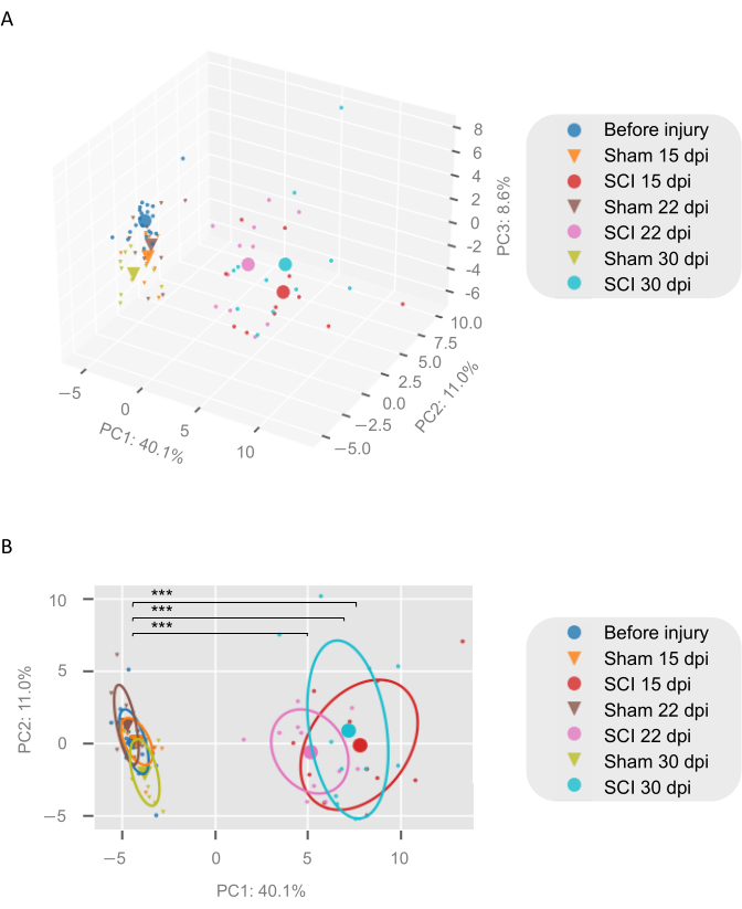
Figure 3: Principal component analysis of all the kinematic motor parameters (79) obtained by the MW software after the residual data analysis. (A) A 3D visualization of the three-component PCA analysis. (B) A 2D visualization with circles representing 50% of collected data. In PC1, which explained over 40% of the variance, the SCI group at 15 dpi, 22 dpi, and 30 dpi was significantly different from the sham group and the baseline (before injury), with a p-value < 0.001, as determined by a one-way ANOVA. Each individual small dot or triangle represents the mean of three videos for each animal, while the larger dots or triangles represent the average point (n = 10-11 per condition, n = 21 for the baseline group). The contribution of each component is indicated in each axis. Abbreviations: dpi = days post-injury; SCI = spinal cord injury; PC = principal component. Please click here to view a larger version of this figure.

Then, a collection of motor parameters was selected based on how strongly it described the dataset (33 in total), and a heatmap was generated (Figure 4). Indeed, most locomotor parameters showed a drastic change after SCI at all time points (15 dpi, 22 dpi, and 30 dpi), while the sham-injured controls only showed significant changes at 30 dpi. These changes in the sham group could be explained by an overall decrease in swing speed, possibly due to test habituation, which will be discussed later.

It was noticeable that the SCI animals walked slower than the sham-injured controls (data not shown). However, independently of speed, at both 15 dpi and 30 dpi, the SCI animals displayed a higher swing duration, lower stance duration, and a lower duty factor index, which relates to the stance duration/stepping period²³. These results indicate that the alterations in leg positioning described above are characteristic of SCI, as seen in other animal models^30,31,32, and are not related to alterations in pace (Figure 4).

It should also be mentioned that the left and right synchrony was not affected, as a significant change in the "phase" indexes for the forelimbs and hindlimbs was not observed^10,23 (Figure 4), indicating intact coupling between the left and right limbs.

Moreover, the SCI mice displayed a lower "stance straightness" index (displacement/path length) in both the forelimbs and hindlimbs (Figure 4). This parameter measures how linear the traces are in relation to the ideal condition, which would be a straight line (ranging from 0 to 1, indicating a linear trace)²⁷. Therefore, these results indicate a strong inability to walk straight in this group.

For each stance phase, the MW draws a reconstruction of the body's oscillations, starting at paw touchdown - the anterior extreme position, or AEP-and ending prior to lift-off - the posterior extreme position, or PEP (see the example in Figure 2C). The "footprint clustering" of both the AEP and PEP measures the standard deviation of the average AEP or PEP coordinates in each video. The SCI animals showed an increase in hindpaw footprint clustering for the AEP at all time points, and a significant effect was only observed for the sham-injured group at 15 dpi (Figure 4). This illustrates that the SCI animals could not correctly position their hindlimbs at touchdown after the swing. Additionally, a decrease in forepaw "footprint clustering" for the PEP was seen, together with a decrease in hindpaw footprint clustering for the PEP, at 30 dpi (Figure 4). These results are in accordance with what is observed in the drawn "stance traces" and suggest that the position of the forepaws becomes more restricted after injury.

Finally, and in accordance with the alterations in the paw positioning, there were alterations in the gait strategies and "pressure" elicited by the paws, as measured by the average brightness over the area (Figure 4), which will be further discussed.

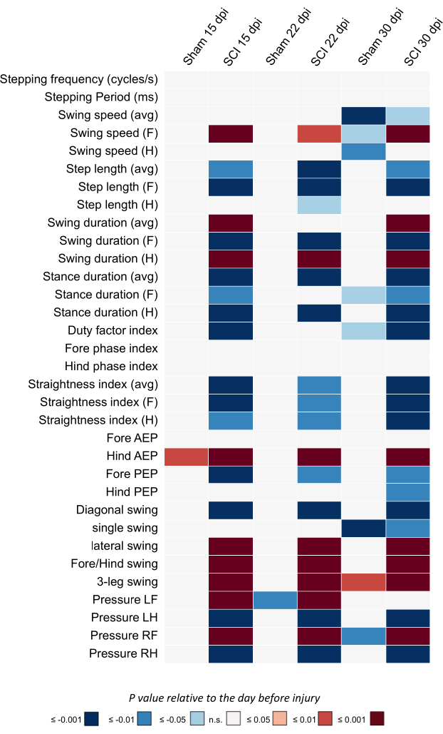
Figure 4: Heatmap plot showing a collection of the significantly altered locomotor parameters comparing SCI animals and sham-injured animals relative to the day prior to surgery, as obtained by the MW after residual data analysis. n = 10-11 per condition; the baseline group includes all the animals the day before surgery, n = 21. Data are expressed by the p-value after statistical analysis with a one-way ANOVA followed by Tukey's post hoc test (for normal distributions) or Dunn's post hoc test (for non-normal distributions). The P-values are represented by a color code, with red and blue shades indicating a decrease or increase relative to baseline, respectively. The color shade represents the statistical significance, with darker colors indicating a higher significance and lighter colors indicating a lower significance; ***P < 0.001; **P < 0.01; *P < 0.05. White indicates no variation. Abbreviations: dpi = days post-injury; SCI = spinal cord injury; s = second; ms = millisecond; avg = average; F = fore; H = hind; AEP = anterior extreme position; PEP = posterior extreme position; LF = left fore; LH = left hind; RF = right fore; RH = right hind. Please click here to view a larger version of this figure.

Subsequently, we sought to understand which individual parameters would be the best to describe the locomotor deficits of SCI animals at different stages of the injury (i.e., 15 dpi, 22 dpi, and 30 dpi). We started by examining the step cycle parameters that showed differences between the forelimbs and hindlimbs as the hindlimbs progressed from total paralysis to partial function (Figure 5). While the average swing speed increased significantly for the forelimbs relative to baseline (before injury), the hindlimb swing speed did not change significantly (although there was a tendency for it to be lower than baseline) (Figure 5A,B). In parallel, the average step length of the forelimbs decreased, with no significant changes for the hindlimbs (Figure 5C,D). Not surprisingly, the injured mice showed decreased forelimb swing duration and an inverse increase in the duration of their hindlimb swings at 15 dpi onward (Figure 5E,F). Taken together, these results indicate that the forelimbs adopted a faster rhythm, with two forelimb cycles for each hindlimb cycle. This 2:1 cycle ratio has been described previously after SCI hemisection in rats^1,33 and illustrates a key aspect of defective forelimb-hindlimb coordination, which is not recovered after 30 dpi in mice.

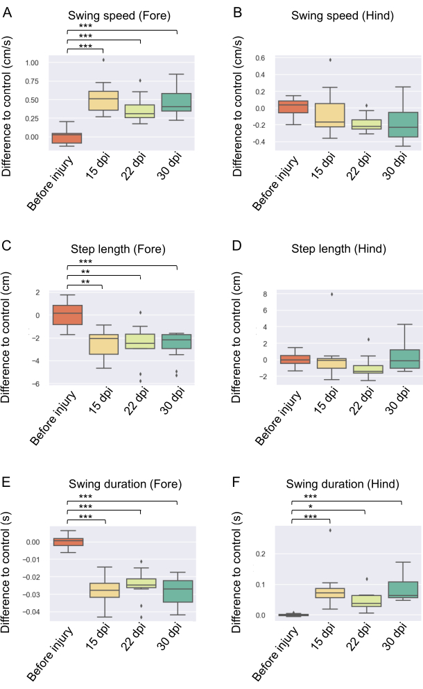
Figure 5: Step cycle parameters for the forepaws and hindpaws at several time points 1 day before the injury and at 15 dpi, 22 dpi, and 30 dpi in SCI animals (n = 11). (A,B) The average swing speed of the forepaws and hindpaws relative to the baseline. (C,D) The average step length of the forepaws and hindpaws relative to the baseline. (E,F) The average swing duration for the forepaws and hindpaws relative to the baseline. In the boxplots, the median is represented by the middle line, and the lower and upper edges of the boxes represent the 25% and 75% quartiles, respectively; the whiskers represent the range of the full data set. Outliers are represented by single dots. Statistical analysis was conducted with a one-way ANOVA followed by Tukey's post hoc test (for normal distributions) or Dunn's post hoc test (for non-normal distributions). *P < 0.05; **P < 0.01; ***P < 0.001. Abbreviations: dpi = days post-injury; SCI = spinal cord injury; cm = centimeter; s = second. Please click here to view a larger version of this figure.

The MW software is also able to compute the stepping patterns of mice by measuring the fraction of frames assigned to a specific leg combination, and this works as a proxy for the presence of specific gait strategies. At slower speeds, uninjured mice tend to adopt a "walking gait", in which most frames have a single-leg swing (regardless of the paw position). At intermediate speeds, most common on the runway, mice change to a trot gait, in which the most representative configuration is the diagonal-leg swing. Finally, at higher speeds, mice use a "gallop gait", with three legs swinging at the same time^23,34. Other less common configurations include the pacing gait, mostly represented by the lateral-leg swing (either both left or right legs), and the "bound/hopping gait", with either both hindlimbs or forelimbs swinging simultaneouslly¹⁰. However, one should keep in mind that, in the context of an SCI, some of these configurations, such as the three-leg swing, can reflect defective hindlimb paw positioning and, thus, do not precisely match with a specific gaiting strategy-in this case, the gallop. Therefore, the analysis was simplified by comparing the leg configurations alone.

After performing the residual analysis, it was noticed that there was a decrease in the prevalence of diagonal swings accompanied by a decrease in single swings at all time points (Figure 6A,B). More interestingly, there was an increase in the prevalence of lateral swings (Figure 6C). The pacing-like gait is not typical for a normal C57BL/6J mouse; however, it has already been reported to occur after SCI hemisection in rats¹. This in-phase pattern was not prevalent enough to change the forelimb or hindlimb phase index (as seen in Figure 3) but illustrates defective spinal feedback from the hindlimbs to the forelimbs. Additionally, there was a natural increase in the prevalence of forelimb/hindlimb swings (Figure 6D), possibly due to incorrect hindlimb plantar stepping, and an increase in three-leg swings (Figure 6E).

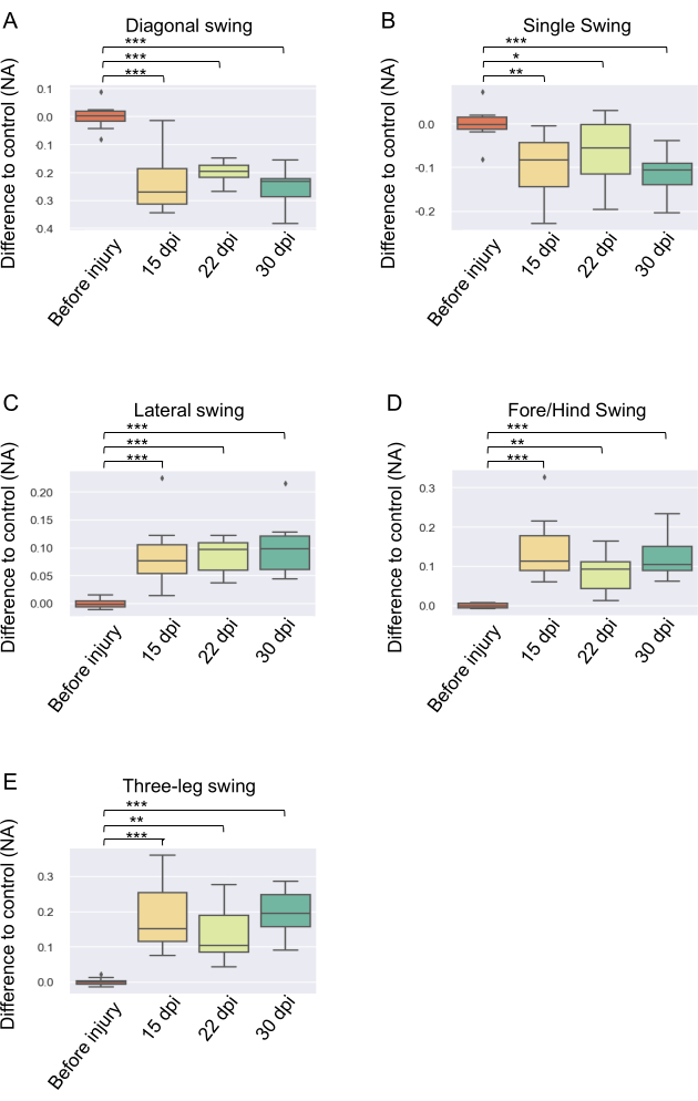
Figure 6: The average indexes for different stepping swing configurations. (A) Diagonal, (B) single, (C) lateral, (D) fore/hind, and (E) three-leg swing at several time points in SCI animals (n = 11) are shown. In the boxplots, the median is represented by the middle line, and the lower and upper edges of the boxes represent the 25% and 75% quartiles, respectively; the whiskers represent the range of the full data set. Outliers are represented by single dots. Statistical analysis was performed with a one-way ANOVA followed by Tukey's post hoc test (for normal distributions) or Dunn's post hoc test (for non-normal distributions). **P < 0.01; ***P < 0.001. Abbreviations: dpi = days post-injury; SCI = spinal cord injury; NA = not applicable. Please click here to view a larger version of this figure.

Finally, another readout that can be extracted from the MW is "pressure" as a measure of brightness/area. With higher speeds, the area of contact with the ground decreases, and the pressure increases, so a linear regression of the baseline data was performed, and the residual values for each condition were measured. It was noticed that the pressure on the forepaws increased significantly across all time points, but the strength of this effect tended to decrease over time, as the change for the left forepaw already lost statistical significance at 30 dpi (Figure 7A,C). This specific effect on the left side could be explained by a lateralized injury, which could have preferentially affected the right side of the spinal cord in this study. Nevertheless, the pressure exerted by the hindpaws was decreased in injured mice, as expected, across all time points, with no tendency toward an increase (Figure 7B,D).

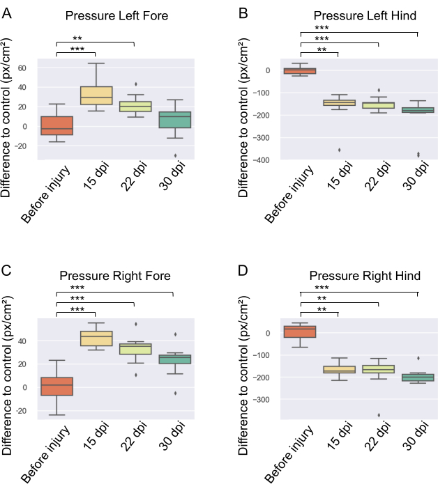
Figure 7: Pressure elicited by the hind and fore paws at several time points in SCI animals (n = 11). Pressure elicited by the (A) left forepaw, (B) left hindpaw, (C) right forepaw, and (D) right hindpaw, shown as relative differences to baseline (the day before injury). In the boxplots, the median is represented as the middle line, and the lower and upper edges of the boxes represent the 25% and 75% quartiles, respectively; the whiskers represent the range of the full data set. Outliers are represented by single dots. Statistical analysis was performed with a one-way ANOVA followed by Tukey's post hoc test (for normal distributions) or Dunn's post hoc test (for non-normal distributions). **P < 0.01; ***P < 0.001. Abbreviations: dpi = days post-injury; SCI = spinal cord injury; cm = centimeter; px = pixel. Please click here to view a larger version of this figure.

Taken together, this study illustrates the power of the MW system for quantitatively describing the motor impairments caused by SCI that can sometimes be disregarded due to other test limitations. Furthermore, it underlines the undoubtedly limited functional recovery across time in the contusion mouse model of SCI.

Supplementary Figure 1: The MW hardware components. (A) This setup is divided as follows: I - fTIR walkway; II - fTIR support base and posts; III - walkway wall; IV - 45° mirror; and V - background backlight. (B) Close-up images of the Base-U- channel and walkway sidelines. (C) Design of the walkway wall. (D) Close-up image of the 45° mirror setup. Abbreviation: cm = centimeter. Please click here to download this File.

Supplementary Figure 2: A single frame of an fTIR video in which the pixel intensity and region areas are indicated. The pixel intensities for the body, background, and footprints used for the video analysis in this study are presented between brackets and indicated in red, all optimized for image clarity. The light intensity should be adjusted to obtain proper discrimination between the different regions. Relative areas of the body and footprints are indicated by dashed yellow lines. Both the areas and pixel intensity were acquired in ImageJ/FIJI. Please click here to download this File.

Supplementary Figure 3: (A) BMS total score and (B) subscore of the mice analyzed in this study (n = 10-11). All data were expressed as mean ± SEM. Statistical analysis was performed with a two-way repeated measures ANOVA followed by Bonferroni's post hoc test; ***P < 0.001. Abbreviation: BMS = Basso mouse scale. Please click here to download this File.

Supplementary Figure 4: The assigned weight of each motor parameter contribution for each component. The assigned weight of each motor parameter (79 in total) after the residual analysis for (A) PC1, (B) PC2, and (C) PC3 in the PCA. The cutoff line was drawn at 0.04 ms and −0.04. Abbreviations: ms = millisecond; avg = average; SD = standard deviation; F = fore; H = hind; AEP = anterior extreme position; PEP = posterior extreme position; LF = left fore; LH = left hind; RF = right fore; RH = right hind; Press = pressure. Please click here to download this File.

Discussion

Here, the potential of the MouseWalker method is demonstrated by analyzing locomotor behavior after SCI. It provides new insights into specific alterations in stepping, footprint, and gait patterns that would otherwise be missed by other standard tests. In addition to providing an updated version of the MW package, data analysis tools are also described using the supplied Python scripts (see step 5).

As the MW generates a large dataset and a collection of kinematic parameters that reflect a highly dimensional locomotor process, a PCA was employed; indeed, PCA has been widely used in other kinematic datasets similar to this one^27,35,36 (Figure 3). This dimensionality reduction technique is a simple and robust method with minimal assumptions that allows for quantitatively identifying kinematic profiles and quickly distinguishing them from control or baseline conditions. In addition, heatmaps were generated to promptly identify the parameters that were statistically different from baseline (Figure 4), which could later be analyzed individually (Figure 5, Figure 6, and Figure 7).

Subsequently, it was shown how specific parameters that can be extracted from the MW illustrate the robust locomotor deficits seen in SCI animals, such as coordination. Coordination is the ability to use each limb in an organized manner to perform a task. Often, coordination is measured indirectly by the number of mistakes/positive events on a ladder^16,17 or the time spent on the rotarod¹⁵. Distinctly, the MW computes both the variability in paw positioning during the step cycle (footprint pattern) and the "stance straightness" index²⁷. It was shown that both parameters were significantly affected by the injury (Figure 4).

Moreover, the MW allows the user to extract parameters related to temporal dynamics. A significant disruption of the swing/stance duration in SCI animals was seen (Figure 4), and it was found that the SCI mice compensated for the loss of support on their hindlimbs by accelerating their forelimb step cycle, thus reducing the forelimb step length and average swing time (Figure 5). This effect could relate to the shift in the center of gravity, which forces the forepaws to endure more body weight¹. Likewise, it could be attributed to the loss of the long ascending propriospinal pathways, which are responsible for the synergetic interaction between the forelimb and hindlimb CPGs^1,9,32, ultimately leading to forelimb-hindlimb rhythm dissociation.

The characteristics of stepping gaits can illustrate the modular organization of locomotor networks^1,34. Although stepping patterns are not a direct proxy for the gait strategies adopted in this case²³, some important observations can still be drawn. Important alterations were seen in the stepping patterns of SCI mice (Figure 6). The injured animals started to adopt lateral swings (pacing-like gaits), and there was also a decrease in diagonal swings. These adaptations seem to be associated with an attempt to coordinate the forelimbs and hindlimbs, again demonstrating the dissociation between the spinal tracks below and above the injury, which does not recover^1,9,32.

The limited recovery after SCI was also verified by a decrease in muscle vigor in the hindlimbs, as measured by the average pressure (Figure 7). Consequently, the forelimbs are forced to support more body weight, which increases the pressure. While many parameters related to muscle dynamics were not analyzed here (i.e., flexor and extensor muscle coordination^7,21), this quantitative measurement can provide a direct read-out of the amount of limb support.

This MW analysis can also be partnered with the standard BMS test, which measures limb rotation, paw placement, tail position, and stepping mistakes. Generally, SCI mice achieve a maximum score of 4-5, with a maximum subscore of 3, meaning they can perform occasional to frequent steps but mostly rotate at the paw lift-off and/or touchdown¹⁴ (Supplementary Figure 2). It becomes clear why the AEP values for the hindpaws were significantly altered in the SCI group, as the non-parallel positioning of the limbs during the swing phase may affect the paw coordinates. In addition, in the BMS, the trunk is usually classified as severe due to the presence of instances or events that prevent stepping, such as butt down and hopping¹⁴. Although it was not possible to quantify butt down behavior or instances that prevented stepping, restricted hindpaw stepping in the MW was detected, with higher swing duration (Figure 5F), increased three leg-swing (Figure 6E), and lower pressure (Figure 7B-D). In addition, a significant increase in fore/hind swings was observed (Figure 6D). There could be two complementary explanations for this behavioral manifestation. First, the hopping-like gait was measured, which could be already observed in the BMS test. However, this behavior could also be related to a lack of correct plantar stepping in both hindlimbs, resulting in foot drag or dorsal placement. Overall, these observations support the claim that trunk stability is severely damaged after SCI. Finally, one of the requirements to score higher than 5 in the BMS test is coordination¹⁴, and for this, at least three accessible passes must be observed by the raters during the test. Of those, two out of the three or more accessible passes need to be classified as coordinated (i.e., forelimbs and hindlimbs alternating). From the MW data, one can extract objective measurements, the stance straightness index, and footprint clustering, which directly quantify coordination independently of animal speed or accessible pass (Figure 4). In addition, the alternation between limbs can be quantified objectively by measuring the stepping strategies (Figure 6). These parameters clearly illustrate that SCI mice consistently cannot walk in straight lines and misplace their hindlimbs.

While the MW toolbox is a helpful strategy for studying locomotor defects after SCI, one should consider some of its limitations. First, it is critical to remain consistent with the acquisition parameters (i.e., camera position, focus, light intensity) so that the image features between time points are maintained. Secondly, it was noticed that repetition led to habituation, which, in turn, led to a decreased speed. This also contributed to increased rearing/grooming behaviors and stops mid-run. For injured animals, there was also a tendency to lean on the walkway walls and an increased number of stops mid-run. As these behaviors are not part of the locomotor assessment, they must not be considered. Preferentially, researchers should choose videos in which the animals walk continuously with their heads pointing straight. To counteract the influence of these behaviors on the results of this study, mice were recorded continuously for at least four or five runs and allowed to run in either direction along the walkway. Afterward, the three best recorded runs were selected and adjusted to the same direction on ImageJ/FIJI²⁴ (180° rotation). Thus, each animal was represented by a mean of three runs pooled together per time point. A larger number of animals per condition could also decrease the expected variability. Moreover, it should be noted that this locomotor test is only recommended after plantar stepping is achieved, as the tracking system was designed for fine-tuned locomotor assessment. In this study, it was noted that before 15 dpi, the MW test was not advantageous for locomotor assessment due to the increased foot drags and incorrect plantar placement, which could affect the tracking (data not shown). Lastly, some parameters (such as footprint clustering) are very sensitive to the extrapolations made by the regression model generated. Therefore, the code was adjusted accordingly (see the documentation in the script in the GitHub link).

Overall, it was shown that the MW could strongly discriminate SCI animals from sham-injured controls, and MW could also be partnered with established tests as a valuable method to study locomotor defects after SCI. Moreover, it was shown that quantitative outputs could be easily generated from the MW dataset using the supplied Python scripts. These tools provide an efficient experimental pipeline to generate a rich and diverse set of quantitative and graphical outputs that complement the original MW output files and can be changed to fulfill the researcher's goals in terms of the type of analysis and graphical representation.

This toolbox is a valuable method for studying other motor-related diseases or motor dysfunctions, not only those related to spinal cord injury. Skarlatou et al.¹⁰ already demonstrated that a specific mutation in Afadin, an important scaffold protein during development, caused an aberrant phenotype in the spinal cord by generating two central canals. This defect resulted in the loss of right-left limb alternation and a higher prevalence of limb synchronization, typical of a hopping gait. Stauch et al.¹⁰ also illustrated that this type of system can be adapted according to user's needs. In this case, it was applied to study specific behavioral deficits in a rat Parkinson's disease model. Thus, this toolbox has a broad range of applications in different models in which motor disturbances are expected and can be combined with already established behavior protocols in the field.

Materials

List of materials used in this article

Name	Company	Catalog Number	Comments
45º Mirror
2 aluminum extrusion (2 x 2 cm), 16 cm height, 1 on each side	Misumi
2 aluminum extrusion (2 x 2 cm), 23 cm, @ 45° , 1 on each side	Misumi
1 aluminum extrusion (2 x 2 cm), 83 cm long	Misumi
87 x 23 cm mirror	General glass supplier
black cardboard filler	General stationery supplier		We used 2, one with 69 x 6 cm and another with 69 x 3cm to limit the reflection on the mirror
Background backlight
109 x 23 cm plexiglass (0.9525 cm thick)	General hardware supplier
2 lateral aluminum extrusion (4 x 4 cm), 20 cm long, 1 on each side	Misumi
multicolor LED strip	General hardware supplier
white opaque paper to cover the plexyglass	General stationery supplier
fTIR Support base and posts
2 aluminum extrusion (4 x 4 cm), 100 cm height	Misumi
60 x 30 cm metric breadboard	Edmund Optics	#54-641
M6 12 mm screws	Edmund Optics
M6 hex nuts and wahers	Edmund Optics
fTIR Walkway
109 x 8.5 cm plexyglass (1.2 cm thick)	General hardware supplier		109 x 8.5 cm plexyglass (1.2 cm thick)
109 cm long Base-U-channel aluminum with 1.6 cm height x 1.9 cm depth thick folds (to hold the plexyglass)	General hardware supplier
2 lateral aluminum extrusion (4 x 4 cm) 20 cm length, 1 on each side	Misumi
black cardboard filler	General stationery supplier		we used 2 fillers on each side to cover the limits of the plexyglass, avoiding bright edges
M6 12 mm screws	Edmund Optics
High speed camera (on a tripod)
Blackfly S USB3	FLIR	#BFS-U3-32S4M-C	This is a reccomendation. The requirement is to record at least 100 frames per second
Infinite Horizon Impactor
Infinite Horizon Impactor	Precision Systems and Instrumentation, LLC.	#0400
Lens
Nikon AF Zoom-Nikkor 24-85mm	Nikon	#1929	This lens is reccomended, however other lens can be used. Make sure it contains a large aperture (i.e., smaller F-stop values), to capture fTIR signals
Software
MATLAB R2022b	MathWorks
Python 3.9.13	Python Software Foundation
Anaconda Navigator 2.1.4	Anaconda, Inc.
Spyder 5.1.5	Spyder Project Contributors
Walkway wall
2 large rectagular acrilics with 100 x 15 cm	Any bricolage convenience store
2 Trapezian acrilic laterals with 6-10 length x 15 cm height	Any bricolage convenience store
GitHub Materials
Folder name	URL
Boxplots	https://github.com/NeurogeneLocomotion/MouseWalker/tree/main/Boxplots		Script to create Boxplots
Docs	https://github.com/NeurogeneLocomotion/MouseWalker/tree/main/Docs		Additional documents
Heatmap	https://github.com/NeurogeneLocomotion/MouseWalker/tree/main/Heatmaps		Script to create heatmap
Matlat script	https://github.com/NeurogeneLocomotion/MouseWalker/tree/main/Matlab%20Script		MouseWalker matlab script
PCA	https://github.com/NeurogeneLocomotion/MouseWalker/tree/main/PCA%20plots		Script to perform Principal Component Analysis
Raw data Plots	https://github.com/NeurogeneLocomotion/MouseWalker/tree/main/Rawdata%20Plots		Script to create Raw data plots
Residual Analysis	https://github.com/NeurogeneLocomotion/MouseWalker/tree/main/Residual_Analysis		Code to compute residuals from Raw data

References

- Frigon, A. The neural control of interlimb coordination during mammalian locomotion. Journal of Neurophysiology. 117 (6), 2224-2241 (2017).
- Grillner, S. Biological pattern generation: The cellular and computational logic of networks in motion. Neuron. 52 (5), 751-766 (2006).
- Dominici, N., et al. locomotor primitives in newborn babies and their development. Science. 334 (6058), 997-999 (2011).
- Courtine, G., et al. Kinematic and EMG determinants in quadrupedal locomotion of a non-human primate (Rhesus). Journal of Neurophysiology. 93 (6), 3127-3145 (2005).
- Clarac, F., Cattaert, D., le Ray, D. Central control components of a 'simple' stretch reflex. Trends Neuroscience. 23 (5), 199-208 (2000).
- Squair, J. W., Gautier, M., Sofroniew, M. V., Courtine, G., Anderson, M. A. Engineering spinal cord repair. Current Opinion in Biotechnology. 72, 48-53 (2021).
- Wenger, N., et al. Spatiotemporal neuromodulation therapies engaging muscle synergies improve motor control after spinal cord injury. Nature Medicine. 22 (2), 138-145 (2016).
- Grillner, S. The spinal locomotor CPG: A target after spinal cord injury. Progress in Brain Research. 137, 97-108 (2002).
- Boulain, M., et al. Synergistic interaction between sensory inputs and propriospinal signalling underlying quadrupedal locomotion. Journal of Physiology. 599 (19), 4477-4496 (2021).
- Skarlatou, S., et al. Afadin signaling at the spinal neuroepithelium regulates central canal formation and gait selection. Cell Reports. 31 (10), 107741(2020).
- Viala, D., Vidal, C. Evidence for distinct spinal locomotion generators supplying respectively fore-and hindlimbs in the rabbit. Brain Research. 155 (1), 182-186 (1978).
- Silver, J., Miller, J. H. Regeneration beyond the glial scar. Nature Reviews Neuroscience. 5 (2), 146-156 (2004).
- Basso, D. M., Beattie, M. S., Bresnahan, J. C. A sensitive and reliable locomotor rating scale for open field testing in rats. Journal of Neurotrauma. 12 (1), 1-21 (1995).
- Basso, D. M., et al. Basso mouse scale for locomotion detects differences in recovery after spinal cord injury in five common mouse strains. Journal of Neurotrauma. 23 (5), 635-659 (2006).
- Jones, B. J., Roberts, D. J. The quantitative measurement of motor inco-ordination in naive mice using an accelerating rotarod. Journal of Pharmacy and Pharmacology. 20 (4), 302-304 (1968).
- Metz, G. A., Whishaw, I. Q. The ladder rung walking task: A scoring system and its practical application. Journal of Visualized Experiments. (28), e1204(2009).
- Metz, G. A., Whishaw, I. Q. Cortical and subcortical lesions impair skilled walking in the ladder rung walking test: A new task to evaluate fore-and hindlimb stepping, placing, and coordination. Journal of Neuroscience Methods. 115 (2), 169-179 (2002).
- Wallace, J. E., Krauter, E. E., Campbell, B. A. Motor and reflexive behavior in the aging rat. Journal of Gerontology. 35 (3), 364-370 (1980).
- Carter, R. J., et al. Characterization of progressive motor deficits in mice transgenic for the human Huntington's disease mutation. The Journal of Neuroscience. 19 (8), 3248-3257 (1999).
- Leblond, H., L'espérance, M., Orsal, D., Rossignol, S. Behavioral/systems/cognitive treadmill locomotion in the intact and spinal mouse. The Journal of Neuroscience. 23 (36), 11411-11419 (2003).
- Courtine, G., et al. Recovery of supraspinal control of stepping via indirect propriospinal relay connections after spinal cord injury. Nature Medicine. 14 (1), 69-74 (2008).
- Hamers, F. P. T., Koopmans, G. C., Joosten, E. A. J. CatWalk-assisted gait analysis in the assessment of spinal cord injury. Journal of Neurotrauma. 23 (3-4), 537-548 (2006).
- Mendes, C. S., et al. Quantification of gait parameters in freely walking rodents. BMC Biology. 13 (1), 50(2015).
- Schindelin, J., et al. Fiji: An open-source platform for biological-image analysis. Nature Methods. 9 (7), 676-682 (2012).
- Stauch, K. L., et al. Applying the ratwalker system for gait analysis in a genetic rat model of Parkinson's disease. Journal of Visualized Experiments. (167), e62002(2021).
- Mendes, C. S., Rajendren, S. V., Bartos, I., Márka, S., Mann, R. S. Kinematic responses to changes in walking orientation and gravitational load in Drosophila melanogaster. PLoS One. 9 (10), e109204(2014).
- Cabrita, A., et al. Motor dysfunction in Drosophila melanogaster as a biomarker for developmental neurotoxicity. iScience. 25 (7), 104541(2022).
- Bishop, C. M. Pattern Recognition and Machine Learning. , Springer. Delhi, India. (2006).
- vander Maaten, L., Postma, E., vanden Herik, J. Dimensionality reduction: A comparative review. , Tilburg University. The Netherlands.. http://www.uvt.nl/ticc (2009).
- Courtine, G., et al. Performance of locomotion and foot grasping following a unilateral thoracic corticospinal tract lesion in monkeys (Macaca mulatta). Brain. 128 (10), 2338-2358 (2005).
- Drew, T., Jiang, W., Kably, B., Lavoie, S. Role of the motor cortex in the control of visually triggered gait modifications. Canadian Journal of Physiology and Pharmacology. 74 (4), 426-442 (1996).
- Cheng, H., et al. Gait analysis of adult paraplegic rats after spinal cord repair. Experimental Neurology. 148 (2), 544-557 (1997).
- Thibaudier, Y., et al. Interlimb coordination during tied-belt and transverse split-belt locomotion before and after an incomplete spinal cord injury. Journal of Neurotrauma. 34 (9), 1751-1765 (2017).
- Bellardita, C., Kiehn, O. Phenotypic characterization of speed-associated gait changes in mice reveals modular organization of locomotor networks. Current Biology. 25 (11), 1426-1436 (2015).
- Machado, A. S., Marques, H. G., Duarte, D. F., Darmohray, D. M., Carey, M. R. Shared and specific signatures of locomotor ataxia in mutant mice. eLife. 9, 55356(2020).
- Takeoka, A., Vollenweider, I., Courtine, G., Arber, S. Muscle spindle feedback directs locomotor recovery and circuit reorganization after spinal cord injury. Cell. 159 (7), 1626-1639 (2014).
Reprints and Permissions