Comprehensive Characterization of Tissue Mineralization in an Ex Vivo Model

Summary

The proposed protocol entails a global approach to assess bone formation in the context of bone regeneration using multimodal analyses. It aims to provide qualitative and quantitative information on new bone formation, enhancing the rigor and validity of basic and pre-clinical investigations.

Abstract

The extensive characterization of tissue mineralization in the context of bone regeneration represents a significant challenge, given the numerous modalities that are currently available for analysis. Here, we propose a workflow for a comprehensive evaluation of new bone formation using a relevant large animal osseous ex vivo explant. A bone defect (diameter = 3.75 mm; depth = 5.0 mm) is created in an explanted sheep femoral head and injected with a macroporous bone substitute loaded with a pro-osteogenic growth factor (bone morphogenetic protein 2 - BMP2). Subsequently, the explant is maintained in culture for a 28-day period, allowing cellular colonization and subsequent bone formation. To evaluate the quality and structure of newly mineralized tissue, the following successive methods are set up: (i) Characterization and high-resolution 3D images of the entire explant using micro-CT, followed by deep learning image analyses to enhance the discrimination of mineralized tissues; (ii) Nano-indentation to determine the mechanical properties of the newly formed tissue; (iii) Histological examinations, such as Hematoxylin/Eosin/Saffron (HES), Goldner's trichrome, and Movat's pentachrome to provide a qualitative assessment of mineralized tissue, particularly with regard to the visualization of the osteoid barrier and the presence of bone cells; (iv) Back-scattering scanning electron microscopy (SEM) mapping with internal reference to quantify the degree of mineralization and provide detailed insights into surface morphology, mineral composition, and bone-biomaterial interface; (v) Raman spectroscopy to characterize the molecular composition of the mineralized matrix and to provide insights into the persistence of BMP2 within the cement through the detection of peptide bonds. This multimodal analysis will provide an effective assessment of newly formed bone and comprehensive qualitative and quantitative insights into mineralized tissues. Through the standardization of these protocols, we aim to facilitate interstudy comparisons and improve the validity and reliability of research findings.

Introduction

Bone defects, whether caused by trauma, tumor resection, congenital anomalies, or infection, represent a major challenge for regenerative medicine. These alterations compromise the structural integrity of the skeletal system, leading to discomfort, functional impairment, and a reduction in patients' quality of life.

To overcome these challenges, innovative bone repair strategies have emerged, with a focus on enhancing osteogenesis and bone tissue regeneration. These approaches include the use of implantable, injectable, or 3D-printable bone substitutes, which can be of natural origin (e.g., bio-sourced macromolecules, animal-derived hydroxyapatite) or synthetic (e.g., bioglasses, calcium phosphates)¹. To enhance their low inherent ability to guide and stimulate bone regeneration, bone substitutes can be loaded with osteoinductive factors, such as bone morphogenetic proteins (BMPs), to promote osteogenic differentiation of progenitor cells and enhance bone formation².

Bone formation is based on the initial formation of a collagen matrix, which is then mineralized by hydroxyapatite crystals, thereby reinforcing the bone structure³. This process confers specific stiffness and strength to the bone. The quality of the mineralized tissue is intricately governed by its microstructural attributes and degree of mineralization⁴. This quality plays a pivotal role in bone healing and the functionality of the regenerated bone⁵. However, characterizing bone mineralization remains a challenging task due to the inherent variability across multivariate studies^6,7,8.

In addition, initial evaluations of the biocompatibility, cytocompatibility, and differentiation potential of bone graft substitutes are typically conducted in vitro. However, methodological disparities impede the seamless comparison of outcomes. Furthermore, these in vitro studies do not fully capture the multicellular interactions and complex dialogue between cell populations, including bone marrow cells, which are essential for regulating the bone regeneration process⁹. This lack of accurate representation of the bone microenvironment may compromise the accuracy of subsequent preclinical studies¹⁰.

Although in vivo assessments provide a more accurate representation of physiological contexts, they are constrained by ethical, logistical, and financial considerations. Consequently, ex vivo evaluations play a pivotal role as an interface between in vitro and in vivo studies, serving as a necessary intermediate step before moving on to experiments on living subjects^11,12,13.

In this context, the implementation of comprehensive characterization methodologies is needed to appraise the quality of regenerated bone tissue and to ensure the relevance of the strategy before moving on to a preclinical model. Consequently, we propose a protocol based on the analysis of an explant model using sheep knee joint tissue. This innovative methodology involves implanting BMP2-loaded cement into the explants and conducting a detailed analysis of tissue mineralization after 28 days of culture.

The technical approaches employed in this study are diverse and complementary, collectively providing a comprehensive approach to evaluating the quality of regenerated bone tissue (Figure 1). High-resolution micro-CT imaging enables detailed 3D visualization of the bone structure, providing valuable insights into the mineral density, morphology, and integrity of the newly formed tissue. This technique is crucial for assessing the efficacy of bone regeneration and monitoring the progression of mineralization over time. Nanoindentation is a precise approach for determining the mechanical properties of the tissue, such as its hardness and strength. By measuring the response of the material to a force applied on a nanometric scale, this method enables the assessment of the robustness and quality of the mineralized tissue. Histological examinations using common staining such as hematoxylin/eosin/saffron (HES), Goldner's trichrome, and Movat's pentachrome provide invaluable insights into tissue structure and composition. These stainings' allow differentiation of the various tissue components, including cells, extracellular matrix, and mineral deposits, thereby enabling a comprehensive qualitative assessment of the bone regeneration process. Backscatter scanning electron microscopy (SEM) mapping offers a high-resolution visualization of the surface of the samples, allowing detailed analysis of the degree of mineralization of the bone matrix, as well as the interfaces between the implanted material and the host tissue. Finally, Raman spectroscopy provides information regarding the molecular composition of the tissue, particularly through the identification of specific components such as proteins, lipids, and minerals. This approach enables the characterization of the mineralized matrix and the detection of growth factors such as BMP2, thereby providing crucial information on the persistence of pro-osteogenic stimuli in the regeneration medium.

Using a multi-disciplinary approach, integrating various analytical techniques, our study aims to provide a thorough and comprehensive assessment of the quality of regenerated bone tissue, thus providing a solid basis for the evaluation of bone graft substitutes and their potential clinical application.

Protocol

This study has been approved by an ethics and animal welfare committee and by the French National Veterinary and Food Administration under number G44171.

1. Preparation and culture of osteochondral explants

1. Harvest sheep joint specimens from freshly euthanized animals in an aseptic environment. Position the sheep in a supine position and shave the left hind limb. Prepare by disinfecting with alcohol around the knee joint. Use lateral parapatellar arthrotomy to expose the anterior and posterior cruciate ligaments, followed by patellar dislocation to reveal the femoral trochlea.
   1. Following tissue harvesting, create a 4.75 mm diameter defect in the lateral condyle using an osteochondral autograft transfer system.
2. Using an orthopedic hammer, create a defect 10 mm in depth and retrieve the explant from the condyle. Subsequently, perform a second defect of 8 mm diameter, centered around the first, using an osteochondral autograft transfer system. This yields osteochondral explants measuring 8 mm x 10 mm, containing a central defect of 4.75 mm x 10.0 mm.
3. If required for logistical reasons, transport the explants in Hank's Balanced Salt Solution (hBSS) supplemented with 1% penicillin-streptomycin and store at 4 °C.
4. Rinse the explants 3x with Phosphate Buffered Saline (PBS), then inject the 4.75 mm x 10.0 mm defect with a calcium phosphate cement supplemented with 40 µg/mL of BMP2. Prepare the cement as described below.
   1. Produce α-tricalcium phosphate (α-TCP) by heat treatment of apatitic tricalcium phosphate rods (isostatic press at 120 MPa) at 1364 °C for a minimum of 12 h, followed by air-quenching¹⁴.
   2. Grind the α-TCP rods in absolute ethanol with a planetary mill ball 2x for 5 min at 500 rpm to produce a fine powder of 13.1 ± 1.7 µm (measured using laser diffraction, as previously described¹⁴).
   3. Sterilize the α-TCP powder by dry heating it at 180 °C for 45 min. Prepare the calcium phosphate cement by mixing α-TCP powder with a 2.5% (w/v) Na₂HPO₄ 0.22 µm filtered solution (liquid/powder ratio of 0.35) for 1 min.
   4. Load the cement paste into a 3 mL syringe prior to injection using an 18 G needle.
5. After 10 min at room temperature (RT), transfer the explants into a 25 cm² flask and gently add 10 mL of complete culture medium consisting of Dulbecco's Modified Eagle Medium (DMEM) high glucose supplemented with 10% fetal bovine serum and 1% penicillin-streptomycin.
6. Maintain the explants for up to 28 days in a 37 °C incubator with 5% CO₂ and change the complete culture medium every 2 days under a laminar flow hood.
7. Rinse the explants 3x with PBS. Transfer them into 50 mL tubes, add 20 mL of 4% paraformaldehyde (PFA), and keep them at 4 °C for 3 days. Then, rinse the explants with PBS and store them in 70% ethanol before subsequent analyses.

2. Micro-CT analysis

1. Conduct micro-tomography analyses utilizing a micro-CT X-ray. Acquire X-ray projections at 10.7 µm resolution, with an exposure time of 1200 ms and a 1 mm aluminum filter (80 kV and 125 µA). Average three images for each 0.45° rotation increment in order to enhance the signal-to-noise ratio.
2. Reconstruct three-dimensional (3D) images using the manufacturer's reconstruction software after an X/Y alignment with a reference scan, with the following parameters - Smoothing: 0, Ring Artefact: 3, Beam Hardening: 35%. Clean the image stacks with image processing software and observe with two-dimensional (2D) and 3D visualization tools.

3. Deep-learning image analyzes

1. Conduct image segmentation using dedicated specialized software. Use the integrated segmentation Wizard to train a deep-learning model for bone and cement discrimination.
2. Select a representative zone (i.e., frame) containing bone, cement, and background from the reconstructed micro-CT images. Segment this first frame manually using either simple (e.g., threshold) or powerful tools (e.g., propagation) provided by the software .
3. Generate a deep learning model in the Model tab and select 3D-Unet Routine in the drop-down menu. Define its experimental parameters in adequation with the images to analyze by a right click on the generated model; here: depth of 5, patch size 32 x 32, Adadetla algorithm, stride ratio of 0.25, data augmentation x10.
4. Use the segmented frame to train the deep-learning routine (click on the Train Button), which is acknowledged to be relevant for its fast and accurate image segmentation capabilities^3,15. Once the training is completed, define a second work zone (frame) and automatically segment using the predict function.
   1. Apply manual correction if required to generate more accurate training data. Train routine once again. Repeat the process until a satisfactory result is obtained; the number of data augmentations progressively decreases as the number of training frames increases.
      NOTE: The DICE index provided during the model training gives an indication of the accuracy of the model (compared to the input information) but is not sufficient. Confirmation of the relevance of the model should be carried out by validation of the automatically segmented data by 3 independent seasoned researchers.
5. Publish the model by clicking on the Export button and apply it to the entire micro -CT dataset by clicking Segment > Exported Model > Segment Full Dataset.

4. Embedding

1. Dehydrate the bone explants by placing them in a 40 mL glass vial containing 25 mL of dehydration solution composed of 70% acetone and 30% xylene. Place the glass vial on a rotating wheel for 1 h at RT. Repeat this step 3x.
2. Replace the dehydration solution with 25 mL of xylene and place the glass vial on the rotating wheel for 1 h at RT.
3. Replace the xylene solution with 25 mL of methylmethacrylate enriched (MMA) with 10% benzoyl peroxide (BPO) and 10% dibutyl phthalate (DBP). Place it on the rotating wheel for 1 h at RT. Repeat this step 2x.
4. Replace the MMA solution with 25 mL of MMA enriched with 10% BPO, 10% DBP, and 450 µL of N, N dimethylaniline diluted 1:20 in propan-2-ol. Place the glass vial at -20 °C overnight. The solution becomes yellowish.
5. Place the explant into a medium-size embedding mold and pour the MMA-BPO-DBP-N, N aniline into the mold. Place the mold into a plastic box and ventilate with nitrogen flow for 5 min. Close the box hermetically and place it at 4 °C for 48 h for MMA polymerization and hardening.
6. Remove the resin containing the explant from the mold and keep it at 4 °C until processed for subsequent analysis.

5. Scanning electron microscopy (SEM) - quantitative backscattered electron imaging (qBEI)

1. Cut the pMMA block containing the explant with a diamond saw along its long axis. Keep the first half of the block for histological analysis. Cut the other half further to generate a 1.5 mm thick section. Perform the cut at 3000 rpm with a 3 mm/min speed.
2. Grind the section with silicon carbide paper with ascending numbers corresponding to lower grain size: SiC 320 for 10 s, SiC 1000 for 15 s, SiC 2000 for 30 s, and SiC 4000 for 30 s.
3. Polish the section with diamond paste and specific clothes: polishing cloth with 3 µm Mol B3 diamond solution for 1 min and fleece cloth with 1 µm Nap B1 diamond solution for 1 min.
4. Rinse the section under double distilled water and clean off diamond particles with a cotton bud. Dry the section under nitrogen gas.
5. Carbon coat the thick section (10 nm carbon film thickness) and mount it on an aluminum stub with silver paint. Make a silver paint bridge between the section top and the stub to allow for electron charging evacuation to the ground.
6. Place the stub on the SEM stage. Next to the sample, insert a control stub composed of a Faraday cup with carbon, aluminum, and silicon standards into the SEM chamber. This will be used to calibrate the electron beam and convert the grey levels into percentages of Ca. Close the SEM chamber and vacuum.
7. Turn on the electron beam and adjust SEM parameters to run in the backscattered electron mode. On backscattered images, the grey level of the carbon standard is 25, the aluminum standard is 225, and the silicon standard is 253. As an indication, on the system used, SEM parameters are accelerating voltage 20 keV, probe current measured with the Faraday cup: 250 pA, working distance: 15 mm, aperture: 30 µm, image resolution: 1024 x 768 pixels, vacuum: < 4.10^-4 Pa, dwell time of 100 µs/pixel, brightness ~38 and contrast ~72.
8. When the SEM is calibrated with the standards, acquire images of the specimen in backscattered electron mode.
9. Use the backscattered electron image of the specimen to convert the grey levels to calcium content, as described in Roschger et al.¹⁶. Perform this using any image analysis software.
10. Plot the distribution of calcium content. Calcium content distribution shows a Gaussian distribution. Three main parameters of interest are computed: Ca_mean, as the mean calcium content on the image, Ca_peak as the most frequent calcium concentration encountered on the image and Ca_width as the full width at half maximum of the calcium content distribution.
    NOTE: The reproducibility of qBEi has been investigated by imaging the same region of interest for 5 consecutive days (one acquisition per day). This means that the electron beam was turned on and off between sessions. The error percentage in Ca_mean, Ca_peak, and Cawidth were estimated as 0.5%, 0.7%, and 1.2%, respectively. Calcium content was also investigated by Energy dispersive X-ray analysis (EDS). A very good linear relationship was established between Ca_mean and calcium content estimated by EDS with an R² value of 0.99, similar to data obtained by Roschger et al. previously¹⁷.

6. Histology

1. For each sample, cut 7 µm sections using a hard tissue microtome with a tungsten blade ^18,19. Stain sections with Goldner trichrome, HES, and MOVAT stain using an automatic staining system.
2. For deplastification, soak the samples successively in acetone for 5 min and repeat 2x. Rinse the samples in distilled water for 5 min and repeat 2x.
3. Perform Goldner Trichrome coloration as described below.
   1. Place samples in Weigert ferric hematoxylin for 20 min. Wash with tap water. Immerse samples in 0.5% acid alcohol for 30 s-1 min. Wash with tap water for 20 min.
   2. Place samples in Ponceau/fuchsine acid/azophloxin solution for 5 min. Immerse in 1% acetic acid for 1 min.
   3. Stain with phosphomolybdic acid/Orange G solution for 20 min. Immerse in 1% acetic acid for 1 min.
   4. Stain with fast green solution for 15 min at room temperature or 8 min at 60 °C. Rinse thoroughly with tap water; repeat 3x.
4. Perform Movat Pentachrome coloration as described below.
   1. Alcian Blue staining: immerse samples in Alcian Blue solution for 30 min. Rinse samples in tap water for 5 min. Place samples in alkaline ethanol for 60 min. Rinse samples in tap water for 10 min. Perform a final rinse with distilled water.
   2. Weigert Hematoxylin staining: place samples in Weigert's Ferric Hematoxylin for 20-30 min. Rinse samples in tap water for 15 min. Rinse again with distilled water.
   3. Staining with Crocein Brilliant/fuchsine acid: immerse the samples in a solution of Crocein Brilliant/Acid Fuchsin for 10 min. Rinse with 0.5% acetic acid. Immerse samples in a 5% phosphotungstic acid solution for 20 min. Rinse with 0.5% acetic acid for 2 min. Perform three successive rinses with 100% ethanol, each lasting 5 min.
   4. Staining with Safran du Gatinais: place samples in Safran du Gatinais for 15 min. Perform a final rinse with tap water.
5. Perform HES coloration as described below.
   1. Staining with Weigert's Hematoxylin: submerge the samples in Weigert's Hematoxylin for 30 min. Rinse with tap water for 2 min.
   2. Decolorization: dip the samples in hydrochloric acid alcohol for 10 s. Rinse with tap water for 2 min.
   3. Neutralization: immerse the samples in a solution of lithium carbonate for 1 min. Rinse with tap water for 2 min. Perform a final rinse with distilled water for 1 min.
   4. Staining with Eosin-Erythrosine: place the samples in a solution of Eosin-Erythrosine for 3 min. Rinse with tap water for 10 s.
   5. Dehydration: Submerge the samples in 95% alcohol for 15 s. Transfer to 100% alcohol for 15 s. Repeat the immersion in 100% alcohol for 30 s.
   6. Final staining with Alcoholic Safranin: immerse the samples in alcoholic safranin for 10 min. Perform a final rinse with tap water.
6. Perform slide mounting as described below.
   1. Rinse samples in 95% ethanol, then 100% ethanol, then methylcyclohexane and repeat this 3x for each step.
   2. Mount the samples using a mounting kit and add a coverslip. Scan the images using a digital slide scanner.

7. Raman microspectroscopy

1. Use the same section used for Raman analysis as the SEM. Briefly grind and polish the section as described in steps 5.2 - 5.3 to remove the thin carbon layer added for SEM that impairs heat dissipation from the sample.
2. Place the section on the stage of the Raman microspectrometer. Calibrate the wavenumber to ensure accuracy and align the laser prior to measurement. As such procedures are specific to each instrument, they will not be described in this article.
3. Locate regions of interest in the tissue that need to be analyzed. Position the zone to be analyzed in the center of the video tool and collect Raman spectra with the following parameters: 785 nm laser used at 30 mW, time of integration: 20 s repeated 3 times, spectral range: 350-1800 cm^-1, grating 1200 lines/mm.
4. Collect 10 spectra of the embedding resin with the same Raman settings and average them. Use this to subtract the resin contribution in step 7.6.
5. Pre-process the spectra as follows to remove the contribution of fluorescence, noise, and resin: baseline correction with a five-order polynomial fitting, Savitzky-Golay filter with a degree of 4, and a window size comprised between 17 and 21, digital resin subtraction using the ~812 cm^-1 peak of the resin. Such pre-processing can be performed with different software designed for data analysis and visualization.
6. Further analyze the pre-processed spectra to extract valuable parameters by rationing the peak intensity of the vibration of interest with the peak intensity of the reference vibration. For bone analysis, for example, use the following parameters to compute it.
   1. Mineral-to-matrix ratios: divide the peak intensity of the v1PO4 vibrations at ~960 cm^-1 by the peak intensity of the Amide I (~1668 cm^-1), amide III (~1250 cm^-1), CH2-wag (~1450 cm^-1) or the sum of proline (~854 cm^-1) and hydroxyproline (Hyp, ~872 cm^-1) vibrational modes. The v2PO4, located at ~430 cm^-1, or the v4PO4, located at ~600 cm^-1, can also be used and ratioed with the Amide III vibration²⁰. These parameters represent the degree of mineralization of the organic phase of the bone matrix.
   2. Carbonate/Phosphate: divide the peak intensity of the v1CO₃, located at ~1070 cm^-1, by the v1PO4. This represents the amount of type B carbonate substitution in the apatite lattice. Hyp/Pro, represents the hydroxyproline content, ~1375 cm^-1/Amide III, represents the proteoglycan content, ~1150 cm^-1/CH2-wag and ~1495 cm^-1/CH2-wag, represents the amount of the advanced glycation end products carboxymethylysine and pentosidine, 1670 cm^-1/1690 cm^-1 and 1670 cm^-1/1640 cm^-1 represent the disordered secondary structure of the collagen, also known as collagen maturity, and ordered structures in the form of α-helix in type I collagen, respectively.
7. Evaluate the reproducibility of Raman measurements by examining the same region of interest in 5 consecutive acquisitions (one acquisition a day). For each analyzed parameter, the variance was below 0.2% of the parameter value, supporting good reproducibility. The specificity of each investigated peak has been extensively discussed in the field, and an overview is presented in the recent review of Unal²¹.

8. Nanoindentation

NOTE: Due to the destructive nature of nanoindentation, it is usually performed at the end of the sample analysis routine. The nanoindentation system that we own is equipped with a pyramidal Berkovitch diamond indenter. However, several indenter shapes exist, and no consensus in the literature has been determined for bone or biomaterial specimens.

1. Hydrate the embedded bone specimen in saline for 16 h at RT prior to nanoindentation testing.
2. Calibrate the nanoindentation system using fused silica and record the resulting indentation modulus. For fused silica, the indentation modulus is approximately 72 GPa using a Poisson coefficient of 0.17.
3. Once the nanoindentation system is calibrated, place the sample used for Raman analyses in the optical system of the nanoindentation device to point out locations where nanoindentation will be performed.
   NOTE: This modality varies from one equipment to another; we do not detail how the nanoindentation system and software work but give general advice about the different steps that should be performed.
4. Once the location of nanoindentation is chosen, move the sample under the indentation device and perform indentation. Perform nanoindentation at a constant depth of 900 nm, with a loading/unloading speed of 40 mm/min and 15 s pause between loading and unloading. Set the Poisson coefficient for bone tissue at 0.3.
5. Retrieve the different parameters from the nanoindentation curves and compute them according to Oliver and Pharr's theory²².
   1. Indentation modulus (E_IT) is derived from the known properties of the indentation tip and the reduced modulus and combines the local elastic modulus of the specimen. Compute indentation as:
      
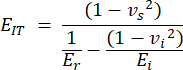
      With v_s, v_i, E_i, and E_r representing the Poisson's coefficient of the sample, assumed to be 0.3 for bone, the Poisson's coefficient of the diamond indenter, assumed to be 0.07, the elastic modulus of the diamond indenter, fixed at 1140 GPa and the reduced modulus, computed as:
      
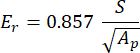
      ​With S representing the slope of the unloading segment and Ap being the projected area and computed as:
      
   2. Hardness (H_IT): corresponding to the bone resistance to initiation and propagation of cracks. In other words, it is an indicator of bone toughness. Compute H_IT as:
      
   3. Indentation creep rate (C_IT): This reflects the bone deformation over time at constant load, indicative of the visco-elastic properties of the specimen, calculate as:
      
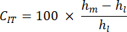
   4. Maximum load (L_m): This corresponds to the opposed loading necessary to penetrate the indicated depth into the mineralized bone matrix.
   5. Indentation work (W_plast): This corresponds to the area under the load/unload deformation curve. It is a direct reflection of the energy dissipated to induce plastic deformation.
      NOTE: The reproducibility of nanoindentation is more difficult to assess on bone samples due to the destructive nature of this methodology. Nevertheless, we estimated the reproducibility of the standard and uniform fused silica sample. For all of the above parameters, the variance was estimated below 0.26% (5 consecutive measures on 5 separate days), supporting very good reproducibility. On the other hand, due to the anisotropic nature of bone samples, it is more difficult to appreciate their reproducibility.

Results

A micro-CT image of the explant is shown in Figure 2. Using Manual segmentation cannot optimally separate bone from cement, present in the central canal, using global thresholding. To improve the recognition of trabecular bone and cement, we propose to use deep learning. Deep learning is powerful for recognizing biomaterial characteristics and helps to improve the separation between bone and cement, enabling a better assessment of cement-bone interactions. This is of the utmost importance in order to accurately quantify the amount of bone formed at the interface with cement and not to incorporate false pixels in this calculation.

However, simply quantifying bone at the interface is not enough to characterize newly formed bone. A more in-depth study of bone matrix quality and cellular composition is required to better understand the strength of the new bone and the cellular mechanisms that led to the formation of this new matrix. The bone matrix can be characterized using two complementary approaches: qBEI and Raman microspectroscopy. An example of a qBEI image is presented in Figure 3. With qBEI, each grayscale-encoded pixel is transformed into a calcium concentration. This is a prerequisite for assessing the distribution of calcium content in trabecular bone and for understanding (i) the degree of mineralization of newly-formed bone at the interface with cement and (ii) whether the presence of cement disrupts trabecular bone mineralization. The advantage of qBEI is its ability to acquire a high-resolution image in a very short time, unlike Raman microspectroscopy which requires a longer acquisition time. qBEI parameters such as Ca_mean, Ca_peak and Ca_width can then be derived from the calcium distribution and used to compare the response between two cements or biomaterials.

On the other hand, qBEI does not provide any information on the quality of the organic phase of the bone matrix at the interface with the biomaterial. Additional information regarding the material properties of the organic phase is derived from Raman microspectroscopy. Raman microspectroscopy is performed on the same specimen as used for qBEI after a quick surface grinding and polishing in order to remove the conductive carbon layer. In Raman microspectroscopy, spectra are acquired at each pixel location. Examples of raw unprocessed and processed Raman spectra are provided in Figure 4. Each spectrum contains information on the composition of the pixel analyzed and includes peaks related to the embedding resin, in this case, pMMA, the mineral phase, peaks v1PO4 and v1CO3, and the organic phase, peaks Pro, Hyp, CML, Amide III, PG, CH2, Pen. and Amide I. In the example in Figure 4, the untreated spectrum shows the contribution of the coating resin at ~812 cm^-1 and a non-zero curved baseline due to fluorescence, although a near-infrared red laser is used. Spectrum processing is a prerequisite for ensuring accurate calculation of the various Raman parameters, in particular the elimination of background fluorescence. When acquiring data, the user should ensure both accurate positioning and avoidance of detector saturation to confirm the presence of the v1PO4 peak located ~960 cm^-1. Following post-processing, peak intensity ratios are computed according to the location of the characteristic vibrational mode.

However, it is questionable whether changes in material composition led to changes in biomechanical response. To gather information on the biomechanics of newly formed bone, we systematically carry out nanoindentation investigations on the same sample used for Raman microspectroscopy. Tissue mechanical information is obtained from nanoindentation curves represented by load versus depth curves (Figure 5). It is worth noting that the depth does not go back to zero at the end of the test, representing the plastic deformation and the permanent damage created to the material. The indentation creep rate is derived from the depth versus time curve.

Finally, histological staining is used to assess the tissue response to the biomaterial at the cellular level (Figure 6). The histological stains proposed allow us to determine the presence of osteoid tissue, but also the identification of cells (macrophages, multinucleated giant cells, osteoclasts, osteoblasts) and the possible presence of a fibrous capsule at the interface with the biomaterial. This is very important for understanding the biocompatibility of a biomaterial, but also the persistence of new bone when the biomaterial is degraded.

Overall, the multi-method approach enables an in-depth study of bone formation, the quality of newly formed bone, and cellular composition. When carried out in the proposed sequential order, all investigations can be performed on the same sample, reducing cost and processing time.

Figure 1: Graphical abstract. A summary of the protocol steps is provided here. Please click here to view a larger version of this figure.

Figure 2: Micro-CT and deep learning analyses. (A) 3D reconstruction of micro-CT images. (B) Bone and cement segmentation: comparison between manual segmentation and deep learning. Scale bar = 5 cm. Please click here to view a larger version of this figure.

Figure 3: Quantitative backscattered electron imaging for determining calcium content. (A) The backscattered image composed of grey levels obtained in the scanning electron microscopy (SEM) is converted by the image analysis software into (B) a calcium map showing the hot spots of the bone sample. (C) The distribution of the calcium content versus bone area is plotted, and the three major qBEI parameters, Camean, Capeak, and Ca_width, are computed. Please click here to view a larger version of this figure.

Figure 4: Example of Raman spectra. (A) Raw unprocessed Raman spectrum obtained in the spectral range 800 - 1800 cm^-1. The fluorescence background is clearly visible as the spectra do not start from 0. The resin contribution (pMMA) is clearly visible at ~812 cm^-1. (B) Processed spectrum. The position of the different vibrational modes of interest is indicated on the spectrum. Please click here to view a larger version of this figure.

Figure 5: Investigation of tissue mechanical properties by nanoindentation. (A) The nanoindentation device is composed of an optical part used to define the location of the region of interest at the surface of the specimen block, and then the block is translated under the indentation part. (B) Load versus time and depth versus time are plotted during indentation test and are used to generate the (C) load versus depth curve. In this example the chosen depth was fixed at 400 nm. The maximum load (L_m), the depth at the end of loading (h_l), the depth after the pause period (h_m), the slope of the unloading segment (S) and the area under the loading-unloading phase of the test (W_plast) are derived from the load versus depth curve and are used to compute the different nanoindentation parameters. Please click here to view a larger version of this figure.

Figure 6: Histological analysis of osteochondral explants treated with cement after 28 days of culture. (A) Movat staining demonstrates the tissue structure, including bone and the cement filling the defect. (B) HES staining illustrates the tissue integration and cellular response around the cement. Scale bar: 2.5 mm. (C) Magnification of the highlighted area in (B), which details the interface between the cement and the surrounding tissue, where cells can be observed invading the cement. Scale bar: 500 µm. Please click here to view a larger version of this figure.

Discussion

Repair of bone defects is a major challenge in regenerative medicine to restore mobility, reduce pain, and improve the quality of life of affected individuals. The use of explant models offers a number of advantages compared to in vivo studies for the investigation of bone defect repair. In addition to ethical considerations, this model allows for the rigorous control of experimental conditions and the reduction of biological variability, thereby facilitating the generation of more accurate and reproducible results. Furthermore, the mechanical and biological properties of sheep bone are closely aligned with those of human bone in comparison to other animals^23,24. This makes the sheep explant model a particularly relevant choice for preclinical studies and a representative model of human clinical conditions.

Along with the development of imaging and material sciences methodology, the explant model described here represents a good model to investigate the effects of regenerative medicine on skeletal tissues in a controlled environment reducing experimental bias. The dimensions and morphology of the explant are optimal for detailed analysis of neo-osteogenesis and material properties, enabling comprehensive assessment and characterization²⁵. These findings emphasize the model's potential for clinical translation, offering a robust framework for evaluating bone graft substitutes and enhancing the likelihood of successful clinical outcomes in bone regeneration therapies. Furthermore, the model facilitates precise evaluation of osteointegration and biomaterial performance, which are critical factors in developing effective bone repair strategies.

To ensure the success of the study, it is critical to follow the protocol's key steps meticulously. One of the most important aspects is ensuring the sample is fully dehydrated during the embedding process. Any remaining moisture can hinder proper resin embedding, leading to a blurred and non-transparent resin, which could compromise the clarity and accuracy of the results and could also result in holes during histology sectioning. This careful attention to detail is essential for producing reliable and reproducible findings. In order to ensure accurate conversion of grey levels into a calcium content map, it is essential to employ calibration using a Faraday cup and C, Al, and Si standards for SEM analysis. It is crucial to ensure consistency in the use of the same SEM for all samples, as differences in backscattered electron detectors can lead to variability in the results. In Raman spectroscopy, calibration of the wavenumber and thorough baseline correction are essential to exclude fluorescence background and differentiate between peaks from the embedding resin and the sample. For nanoindentation, achieving a perfectly smooth surface is critical, given the displacement limits of indenters, and calibration with a known standard, such as fused silica, is necessary to ensure reliable measurements.

The modifications and troubleshooting of these techniques frequently address the anisotropic nature of bone material, which has the potential to influence measurement consistency. To illustrate, in Raman spectroscopy, the polarization of the incident laser can have a considerable impact on the recorded intensity. The use of a 20x objective with a low numerical aperture can assist in the mitigation of this issue. It is also of paramount importance to ensure consistent calibration and measurement conditions across all samples in order to maintain data integrity. The inherent anisotropy of bone represents a limitation of these methodologies, as it can affect the uniformity of measurements, particularly in techniques such as Raman spectroscopy. Furthermore, the necessity for precise calibration and environmental control may limit the general applicability if these aspects are not meticulously managed.

The potential applicability of these approaches extends significantly to the evaluation of novel biomaterials and therapeutic strategies for bone repair. The model's capacity to closely mimic human bone physiology provides a robust platform for preclinical testing, enabling a thorough assessment of the safety and efficacy of new treatments in a controlled setting. This model's utility is particularly relevant for accelerating the translational pathway from laboratory research to clinical practice, facilitating the early identification of promising candidates for bone regeneration therapies. By providing a reliable and reproducible method for evaluating bone repair materials, this technique supports the advancement of regenerative medicine and the development of clinically viable solutions.

Materials

List of materials used in this article

Name	Company	Catalog Number	Comments
0.20 filters	VWR	28145-501
18 G needle (1,2x40 mm)	Sterican	4665120
3 mL syringe	HENKE-JECT	8300005762
37% hydrochloric acid	VWR	1.00317.1000
Acetic acid (glacial)	Sigma	A6283
Acetone	VWR	20063-365
Alcian Blue 8GX	VWR	361186
Ammonium hydroxide	VWR	318612
Apatitic tricalcium phosphate	Centre for Biomedical and Healthcare Engineering (Mines Saint Etienne, France)	TV26U
Azophloxine	Sigma	210633
Benzoyl peroxide	Sigma	8.01641.0250
BMP2	Medtronic	InductOs 1.5 mg/mL
Brillant crocein	Aldrich	2107507
CTVox	Bruker	-
DataViewer	Skyscan	-
Diamond blade	Struers	MOD13
Diamond saw	Struers	Accutom-50
DiaPro Mol B3 diamond solution	Struers	40600379
DiaPro Nap B1 diamond solution	Struers	40600373
Dibasic sodium phosphate (Na2HPO4)	Sigma	102404598
Dibutyl Phtalate	Chimie-Plus Laboratoires	28656
DragonFly software	ORS	2022.1.0.1231.
Dulbecco's Modified Eagle Medium (DMEM) high glucose, GlutaMAX(TM), pyruvate	ThermoFisher Scientific	31966-021
Eosine Y- Surgipath	Sigma	1002830105
Erythrosin B	Sigma	102141057
Ethanol absolute	VWR	20820362
Eukitt	Dutscher	6.00.01.0003.06.01.01
Falcon 50 mL	Sarstedt	62.547.254
Ferric chloride hexahydrate (FeCl3, 6H2O)	Merck	1.03943.0250
Fetal Bovine Serum (FBS)	Eurobio	CVFSVF00
Fuchsine acid	Merck	1.05231.0025
Hank's Balanced Salt Solution (HBSS)	Biosera	MS01NG100J
Hematoxylin	Sigma	86.118.9
Isostatic press	Nova Suisse	Pmax 1500 bars
Laser diffraction granulometry	Malvern	Mastersizer 3000
Light green	Prolabo	28947135
Lithium carbonate	Sigma	A13149
MD-Mol polishing cloth	Struers	40500077
Methylcyclohexane	VWR	8.06147.1000
Methylcyclohexane	VWR	8.06147.1000
Methylcyclohexane	VWR	8.06147.1000
Methylmethacrylate	Sigma	8.00590.2500
Micro-CT, micro-scanner	Bruker	Skyscan 1272
Monobasic sodium phosphate (NAH2PO4)	Sigma	71496
Mortar	Fritsch	Pulverisette 6
N,N, Dimethylanilin	Sigma	803060
Nanoindentation station	Anton Paar	NHT2
ND-Nap polishing cloth	Struers	40500080
OATS Osteochondral Autograft Transfer System Set, 4,75 mm	Arthrex	AR-1981-04S
OATS Osteochondral Autograft Transfer System Set, 8 mm	Arthrex	AR-1981-08S
Orange G	Ral	M15
Paraformaldehyde (PFA)	Sigma	P6148
Peel-a-way disposable embbedding moulds	Polysciences, Inc	18646C-1
Penicillin/Streptomycin (P/S)	ThermoFisher Scientific	15140122
Phosphate Buffered Saline (PBS)	ThermoFisher Scientific	10010023
Phosphomolybdic acid	Sigma	221856-100 g
Phosphotungstic acid	Aldrich	12863-5
Polishing machine	Sturers	Dap V
Poupinel	MEMMERT	TV26U
Raman microspectrometer	Renishaw	InVia Qontor
Safran du Gâtinais	Labonord	11507737
Scanning electron microscope	Carl Zeiss	Evo LS 10
SEM	Zeiss	Carl Zeiss Evo LS10
SiC foils/Grinding papers	Struers	40400008 (#320), 40400011 (#1000), 40400122 (#2000), 40400182 (#4000)
Silver paint	Electron microscopy sciences	12686-15
Standard stub with Faraday cup, carbon, aluminium and silicon standards	Micro-Analysis Consultants Ltd	8602
T25 flask	Corning	430639
Xylene	VWR	28975.325
Xylidine Ponceau	Aldrich	19.976-1

References

- Feroz, S., Cathro, P., Ivanovski, S., Muhammad, N. Biomimetic bone grafts and substitutes: A review of recent advancements and applications. Biomed Eng Adv. 6, 100107(2023).
- Tsuji, K., et al. BMP2 activity, although dispensable for bone formation, is required for the initiation of fracture healing. Nat Genet. 38 (12), 1424-1429 (2006).
- Hadjidakis, D. J., Androulakis, I. I. Boneremodeling. Ann N Y Acad Sci. 1092, 385-396 (2006).
- Boivin, G., Meunier, P. J. The degree of mineralization of bone tissue measured by computerized quantitative contact microradiography. Calcified Tiss Int. 70 (6), 503-511 (2002).
- Boivin, G., et al. Influence of remodeling on the mineralization of bone tissue. Osteoporo Int. 20 (6), 1023-1026 (2009).
- Zanghellini, B., et al. Multimodal analysis and comparison of stoichiometric and structural characteristics of parosteal and conventional osteosarcoma with massive sclerosis in human bone. J Str Biol. 216 (3), 108106(2024).
- Trento, G., et al. formation around two titanium implant surfaces placed in bone defects with and without a bone substitute material: A histological, histomorphometric, and micro-computed tomography evaluation. Clin Implant Dent Relat Res. 22 (2), 177-185 (2020).
- Palmquist, A. A multiscale analytical approach to evaluate osseointegration. J Mater Sci Mater Med. 29 (5), 60(2018).
- Budán, F., et al. Novel radiomics evaluation of bone formation utilizing multimodal (SPECT/X-ray CT) in vivo imaging. PLoS ONE. 13 (9), e0204423(2018).
- Hulsart-Billström, G., et al. A surprisingly poor correlation between in vitro and in vivo testing of biomaterials for bone regeneration: results of a multicentre analysis. Eur Cells Mater. 31, 312-322 (2016).
- Cramer, E. E. A., Ito, K., Hofmann, S. Ex vivo bone models and their potential in preclinical evaluation. Curr Osteoporo Rep. 19 (1), 75-87 (2021).
- Chan, M. E., et al. A trabecular bone explant model of osteocyte-osteoblast co-culture for bone mechanobiology. Cell Mol Bioeng. 2 (3), 405-415 (2009).
- Doke, S. K., Dhawale, S. C. Alternatives to animal testing: A review. Saudi Pharma J. 23 (3), 223-229 (2015).
- Moussi, H., et al. New formulation of injectable and degradable calcium phosphate/silanized hyaluronic acid composite foam: Investigation in a rabbit model of long bone defect. SSRN. , (2024).
- Paré, A., et al. Standardized and axially vascularized calcium phosphate-based implants for segmental mandibular defects: A promising proof of concept. Acta Biomater. 154, 626-640 (2022).
- Roschger, P., Fratzl, P., Eschberger, J., Klaushofer, K. Validation of quantitative backscattered electron imaging for the measurement of mineral density distribution in human bone biopsies. Bone. 23 (4), 319-326 (1998).
- Roschger, P., Plenk, H., Klaushofer, K., Eschberger, J. A new scanning electron microscopy approach to the quantification of bone mineral distribution: backscattered electron image grey-levels correlated to calcium K alpha-line intensities. Scanning Micro. 9 (1), 75-86 (1995).
- Porter, A., et al. Quick and inexpensive paraffin-embedding method for dynamic bone formation analyses. Sci Rep. 7, 42505(2017).
- Goldschlager, T., Abdelkader, A., Kerr, J., Boundy, I., Jenkin, G. Undecalcified bone preparation for histology, histomorphometry and fluorochrome analysis. J Vis Exp. (35), e1707(2010).
- Kazanci, M., Roschger, P., Paschalis, E. P., Klaushofer, K., Fratzl, P. Bone osteonal tissues by Raman spectral mapping: Orientation-composition. J Str Biol. 156 (3), 489-496 (2006).
- Unal, M., Ahmed, R., Mahadevan-Jansen, A., Nyman, J. S. Compositional assessment of bone by Raman spectroscopy. Analyst. 146 (24), 7464-7490 (2021).
- Oliver, W. C., Pharr, G. M. An improved technique for determining hardness and elastic modulus using load and displacement sensing indentation experiments. J Mater Res. 7 (6), 1564-1583 (1992).
- Proffen, B. L., McElfresh, M., Fleming, B. C., Murray, M. M. A comparative anatomical study of the human knee and six animal species. Knee. 19 (4), 493-499 (2012).
- Allen, M. J., Houlton, J. E. F., Adams, S. B., Rushton, N. The surgical anatomy of the stifle joint in Sheep. Vet Surg. 27 (6), 596-605 (1998).
- Kleuskens, M. W. A., van Donkelaar, C. C., Kock, L. M., Janssen, R. P. A., Ito, K. An ex vivo human osteochondral culture model. J Ortho Res. 39 (4), 871-879 (2021).
Access restricted. Please log in or start a trial to view this content.
Reprints and Permissions