Introductory Analysis and Validation of CUT&RUN Sequencing Data

Summary

This protocol guides bioinformatics beginners through an introductory CUT&RUN analysis pipeline that enables users to complete an initial analysis and validation of CUT&RUN sequencing data. Completing the analysis steps described here, combined with downstream peak annotation, will allow users to draw mechanistic insights into chromatin regulation.

Abstract

The CUT&RUN technique facilitates detection of protein-DNA interactions across the genome. Typical applications of CUT&RUN include profiling changes in histone tail modifications or mapping transcription factor chromatin occupancy. Widespread adoption of CUT&RUN is driven, in part, by technical advantages over conventional ChIP-seq that include lower cell input requirements, lower sequencing depth requirements, and increased sensitivity with reduced background signal due to a lack of cross-linking agents that otherwise mask antibody epitopes. Widespread adoption of CUT&RUN has also been achieved through the generous sharing of reagents by the Henikoff lab and the development of commercial kits to accelerate adoption for beginners. As technical adoption of CUT&RUN increases, CUT&RUN sequencing analysis and validation become critical bottlenecks that must be surmounted to enable complete adoption by predominantly wet lab teams. CUT&RUN analysis typically begins with quality control checks on raw sequencing reads to assess sequencing depth, read quality, and potential biases. Reads are then aligned to a reference genome sequence assembly, and several bioinformatics tools are subsequently employed to annotate genomic regions of protein enrichment, confirm data interpretability, and draw biological conclusions. Although multiple in silico analysis pipelines have been developed to support CUT&RUN data analysis, their complex multi-module structure and usage of multiple programming languages render the platforms difficult for bioinformatics beginners who may lack familiarity with multiple programming languages but wish to understand the CUT&RUN analysis procedure and customize their analysis pipelines. Here, we provide a single-language step-by-step CUT&RUN analysis pipeline protocol designed for users with any level of bioinformatics experience. This protocol includes completing critical quality checks to validate that the sequencing data is suitable for biological interpretation. We expect that following the introductory protocol provided in this article combined with downstream peak annotation will allow users to draw biological insights from their own CUT&RUN datasets.

Introduction

The ability to measure interactions between proteins and genomic DNA is fundamental to understanding the biology of chromatin regulation. Effective assays that measure chromatin occupancy for a given protein provide at least two key pieces of information: i) genomic localization and ii) protein abundance at a given genomic region. Tracking the recruitment and localization changes of a protein of interest in chromatin can reveal direct target loci of the protein and reveal mechanistic roles of that protein in chromatin-based biological processes such as regulation of transcription, DNA repair, or DNA replication. The techniques available today to profile protein-DNA interactions are enabling researchers to explore regulation at unprecedented resolution. Such technical advances have been enabled through the introduction of new chromatin profiling techniques that include the development of Cleavage Under Targets and Release Using Nuclease (CUT&RUN) by the Henikoff laboratory. CUT&RUN offers several technical advantages over conventional chromatin immunoprecipitation (ChIP) that include lower cell input requirements, lower sequencing depth requirements, and increased sensitivity with reduced background signal due to a lack of cross-linking agents that otherwise mask antibody epitopes. Adopting this technique to study chromatin regulation requires a thorough understanding of the principle underlying the technique, and an understanding of how to analyze, validate, and interpret CUT&RUN data.

The CUT&RUN procedure begins with binding of cells to Concanavalin A conjugated to magnetic beads to enable manipulation of low cell numbers throughout the procedure. Isolated cells are permeabilized using a mild detergent to facilitate introduction of an antibody that targets the protein of interest. Micrococcal nuclease (MNase) is then recruited to the bound antibody using a Protein A or Protein A/G tag tethered to the enzyme. Calcium is introduced to initiate enzymatic activity. MNase digestion results in mono-nucleosomal DNA-protein complexes. Calcium is subsequently chelated to end the digestion reaction, and short DNA fragments from the MNase digestion are released from nuclei, then subjected to DNA purification, library preparation, and high-throughput sequencing¹ (Figure 1).

In silico approaches to map and quantify protein occupancy across the genome have developed in parallel with the wet lab approaches used to enrich those DNA-protein interactions. Identification of regions of enriched signals (peaks) is one of the most critical steps in the bioinformatics analysis. Initial ChIP-seq analysis methods used algorithms such as MACS² and SICER³, which employed statistical models to distinguish bona fide protein-DNA binding sites from background noise. However, the lower background noise and higher resolution of CUT&RUN data render some peak calling programs employed in ChIP-seq analysis unsuitable for CUT&RUN analysis⁴. This challenge highlights the need for new tools better suited for the analysis of CUT&RUN data. SEACR⁴ represents one such tool recently developed to enable peak calling from CUT&RUN data while overcoming limitations associated with tools typically employed toward ChIP-seq analysis.

Biological interpretations from CUT&RUN sequencing data are drawn from the outputs downstream of peak calling in the analysis pipeline. Several functional annotation programs can be implemented to predict the potential biological relevance of the called peaks from CUT&RUN data. For example, the Gene Ontology (GO) project provides well-established functional identification of genes of interest^5,6,7. Various software tools and resources facilitate GO analysis to reveal genes and gene sets enriched amongst CUT&RUN peaks^{8,9,10,11,12,13,14}. Furthermore, visualization software such as Deeptools¹⁵, Integrative genomics viewer (IGV)¹⁶, and UCSC Genome Browser¹⁷ enable visualization of signal distribution and patterns at regions of interest across the genome.

The ability to draw biological interpretations from CUT&RUN data depends critically upon validation of data quality. Critical components to validate include the assessment of: i) CUT&RUN library sequencing quality, ii) replicate similarity, and iii) signal distribution at peak centers. Completing the validation of all three components is crucial to ensure the reliability of CUT&RUN library samples and downstream analysis results. Therefore, it is essential to establish introductory CUT&RUN analysis guides to enable bioinformatics beginners and wet lab researchers to conduct such validation steps as part of their standard CUT&RUN analysis pipelines.

Alongside the development of wet lab CUT&RUN experiment, various in silico CUT&RUN analysis pipelines, such as CUT&RUNTools 2.0^18,19, nf-core/cutandrun²⁰, and CnRAP²¹, have been developed to support CUT&RUN data analysis. These tools provide powerful approaches to analyzing single-cell and bulk CUT&RUN and CUT&Tag datasets. However, the relatively complex modular program structure and required familiarity with multiple programming languages to conduct these analysis pipelines may hinder adoption by bioinformatics beginners who seek to thoroughly understand the CUT&RUN analysis steps and customize their own pipelines. Circumvention of this barrier requires a new introductory CUT&RUN analysis pipeline that is provided in simple step-by-step scripts encoded using a simple single programming language.

In this article, we describe a simple single-language CUT&RUN analysis pipeline protocol that provides step-by-step scripts supported with detailed descriptions to enable new and novice users to conduct CUT&RUN sequencing analysis. Programs used in this pipeline are publicly available by the original developer groups. Major steps described in this protocol include read alignment, peak calling, functional analysis and, most critically, validation steps to assess sample quality to determine data suitability and reliability for biological interpretation (Figure 2). Furthermore, this pipeline provides users the opportunity to cross-reference analysis results against publicly available CUT&RUN datasets. Ultimately, this CUT&RUN analysis pipeline protocol serves as an introductory guide and reference for bioinformatic analysis beginners and wet lab researchers.

Protocol

NOTE: Information for CUT&RUN fastq files in GSE126612 are available in Table 1. Information related to the software applications used in this study are listed in the Table of Materials.

1. Downloading Easy-Shells_CUTnRUN pipeline from its Github page

1. Open terminal from operating system.
   NOTE: If user is not sure how to open terminal in macOS and Windows, review this webpage (https://discovery.cs.illinois.edu/guides/System-Setup/terminal/). For Linux, review this webpage (https://www.geeksforgeeks.org/how-to-open-terminal-in-linux/).
2. Download the compressed analysis pipeline from Github by typing wget https://github.com/JunwooLee89/Easy-Shells_CUTnRUN/archive/refs/heads/main.zip -O ~/Desktop/Easy-Shells_CUTnRUN.zip in the terminal.
3. After downloading the zip file, decompress the downloaded zip file by typing unzip ~/Desktop/Easy-Shells_CUTnRUN.zip -d ~/Desktop/ in the terminal.
4. After the decompression, delete the zip file by typing rm ~/Desktop/Easy-Shells_CUTnRUN.zip in the terminal and change the folder name by typing mv ~/Desktop/Easy-Shells_CUTnRUN-master ~/Desktop/Easy-Shells_CUTnRUN.
5. After removing the zipped file, type chmod +x ~/Desktop/Easy-Shells_CUTnRUN/script/*.sh in the terminal to set the executable permission for all the shell scripts within the working directory. From now on, just type the path and the name of these shell scripts in terminal or drag the scripts into terminal and enter to run these shell scripts in terminal.
   NOTE: The Bash shell is typically pre-installed on most Linux distributions. However, recent macOS versions no longer provide pre-installed Bash shell. If the system does not have Bash, install Bash shell first. Visit links below for instructions describing how to install the Bash shell in Linux OS (https://ioflood.com/blog/install-bash-shell-linux/) and macOS (https://www.cs.cornell.edu/courses/cs2043/2024sp/styled-3/#:~:text=The first thing you will,you will see the following:). These step-by-step shell scripts are written to create one folder ~/Desktop/GSE126612 to perform most of this CUT&RUN analysis within this directory without any need for modification. If the user understands how to use these shell scripts, users may revise and customize these shell scripts to analyze other CUT&RUN datasets and modify options as per project-specific needs. To read and edit these shell scripts, consider using Visual studio Code (https://code.visualstudio.com/) as one option for an easy-to-use program available for major Operating Systems.

2. Installing the programs required for Easy Shells CUTnRUN

1. Among the shell scripts with the name of Script_01_installation_***.sh, find out the shell script of which name includes operating system type of user's system. Currently, Easy Shells CUTnRUN supports the installation script for macOS, Debian/Ubuntu, and CentOS/RPM-based systems.
2. Open the terminal and type echo $SHELL to check the default shell in the active terminal. If Bash shell is the default shell in current terminal, users may see the following: /path/to/bash (or a similar message such as /bin/bash) in the terminal.
3. If the default shell is not Bash, set Bash shell as default shell by typing chsh -s $(which bash) in the terminal. If the terminal uses Bash shell as default, skip this step.
4. In the terminal, operate the installation shell script by typing ~/Desktop/Easy-Shells_CUTnRUN/scripts/Script_01_installation_***.sh or drag the shell script file into the terminal and enter.
5. Read Test_README.md file in /path/to/SEACR-1.3/Testfiles folder. Follow the instruction within the README file to clarify whether the SEACR in user's system works properly.
   NOTE: It is crucial to validate the SEACR function with test files given by SEACR Github page to obtain proper peak calling results from CUT&RUN data. Therefore, follow the instruction of Test_README.md in /path/to/SEACR-1.3/Testfiles immediately after the SEACR installation. Although Easy Shells CUTnRUN provides installation shell scripts for some operating systems, these scripts may not work in some users' system to install all the programs required for Easy Shells CUTnRUN. If there is any problem in installation, review the original website of the uninstalled program, or request assistance using the Easy Shells CUTnRUN github issues webpage (https://github.com/JunwooLee89/Easy-Shells_CUTnRUN/issues).

3. Downloading the publicly available CUT&RUN dataset from Sequence Read Archive (SRA)

1. Open the terminal and type echo $SHELL to check the default shell in the active terminal. If Bash shell is the default shell in current terminal, users may see the following: /path/to/bash (or a similar message such as /bin/bash) in the terminal.
2. If the default shell is not Bash, set Bash shell as default shell by typing chsh -s $(which bash) in the terminal. If the terminal uses Bash shell as default, skip this step.
3. Type ~/Desktop/Easy-Shells_CUTnRUN/scripts/Script_02_download-fastq.sh in the terminal or drag the shell script file into the terminal and enter.
   NOTE:This script will: (i) Create one folder (~/Desktop/GSE126612/fastq) and download a list of SRA files written in a text file (~/Desktop/Easy-Shells_CUTnRUN/sample_info/SRR_list.txt) within the fastq folder. As an example, the SRR_list.txt includes the fastq files of subset of GSE126612 CUT&RUN samples. (ii) Download the raw fastq files within the fastq folder. (iii) Create one folder (~/Desktop/GSE126612/log/fastq) and write down a log file (download-fastq_log.txt) and downloaded sample information file (SRR_list_info.txt) within this log folder.
4. After running the script, check the log file. If there is any error message within the log file, fix the error and try step 3.3 again. If there is any problem to solve the issue, ask help in Easy Shells CUTnRUN github issues webpage (https://github.com/JunwooLee89/Easy-Shells_CUTnRUN/issues).
   NOTE: To facilitate practice of this CUT&RUN analysis pipeline, the following publicly-available samples are retrieved from SRA: one sample from mock control (IgG), three samples of a chromatin architecture and transcription factor protein (CTCF), four samples corresponding to an 'active' histone mark (H3K27Ac), and three samples corresponding to regions of transcriptional initiation marked by RNA polymerase II (RNAPII-S5P). Sequencing was performed as paired-end, therefore two files are paired per sample.

4. Initial quality check for the raw sequencing files

1. Open the terminal and type echo $SHELL to check the default shell in the active terminal. If Bash shell is the default shell in current terminal, users may see the following: /path/to/bash (or a similar message such as /bin/bash) in the terminal.
2. If the default shell is not Bash, set Bash shell as default shell by typing chsh -s $(which bash) in the terminal. If the terminal uses Bash shell as default, skip this step.
3. Type ~/Desktop/Easy-Shells_CUTnRUN/scripts/Script_03_fastQC.sh in the terminal or drag the shell script into the terminal and enter.
   NOTE: This shell script will: (i) Run FastQC program for all raw fastq files in ~/Desktop/GSE126612/fastq folder and save the quality check report files into the ~/Desktop/GSE126612/fastqc.1st folder. (ii) Write down a log file (fastqc.1st.log.SRR-number.txt) per a FastQC run into a log folder (~/Desktop/GSE126612/log/fastqc.1st).
4. After completion of running the shell script, review the log file to clarify the success of the run. If there is any error message within the log file, correct the error and repeat step 4.3. If there is any problem to solve the issue, request assistance using the Easy Shells CUTnRUN github issues webpage (https://github.com/JunwooLee89/Easy-Shells_CUTnRUN/issues).
   NOTE: Among the output files, fastqc.html files include user-friendly quality check results. If there is severe quality issue(s), discuss with bioinformatics colleagues to determine data suitability for downstream analysis. Similar quality control reports are used to confirm improved data quality after adapter trimming. To use this script for other datasets, edit the path of the working and output directories to meet user's needs. A notable difference when interpreting QC of CUT&RUN compared to ChIP-seq reads is that duplicate reads in CUT&RUN do not necessarily indicate PCR duplicates. This is because recruited MNase will digest in the same or similar locations within experimental groups.

5. Quality and adapter trimming for raw sequencing files

1. Open the terminal and type echo $SHELL to check the default shell in the active terminal. If Bash shell is the default shell in current terminal, users may see the following: /path/to/bash (or a similar message such as /bin/bash) in the terminal.
2. If the default shell is not Bash, set Bash shell as default shell by typing chsh -s $(which bash) in the terminal. If the terminal uses Bash shell as default, skip this step.
3. Type ~/Desktop/Easy-Shells_CUTnRUN/scripts/Script_04_trimming.sh in the terminal or drag the Script_04_trimming.sh script into the terminal and enter.
   NOTE: This shell script will: (i) Run the Trim-Galore program for all the raw fastq files in ~/Desktop/GSE126612/fastq to perform adapter and quality trimming. (ii) Create one folder (~/Desktop/GSE126612/trimmed) and save the Trim-Galore output files within the trimmed folder. (iii) Create one log folder (~/Desktop/GSE126612/log/trim_galore) and write down a log file trim_galore_log_RSS-number.txt per a Trim-Galore run.
4. After completion of the run, review the log file carefully. If there is any error message within the log file, correct the error and repeat step 5.3. If there is any problem to solve the issue, request assistance using the Easy Shells CUTnRUN github issues webpage (https://github.com/JunwooLee89/Easy-Shells_CUTnRUN/issues). 
5. After completion of this process, compare the .html output files with the fastqc.html files created in 4.3. Revise the path of input and output directories to perform the trimming step for any fastq files located elsewhere.

6. Downloading the bowtie2 index for the reference genomes for actual and spike-in control samples

1. Open the terminal and type echo $SHELL to check the default shell in the active terminal. If Bash shell is the default shell in current terminal, users may see the following: /path/to/bash (or a similar message such as /bin/bash) in the terminal.
2. If the default shell is not Bash, set Bash shell as default shell by typing chsh -s $(which bash) in the terminal. If the terminal uses Bash shell as default, skip this step.
3. Type ~/Desktop/Easy-Shells_CUTnRUN/scripts/Script_05_bowtie2-index.sh in the terminal or drag the shell script into the terminal and enter.
   NOTE: This script will: (i) Download Bowtie2 indexes for actual sample reference genomes (human; hg19; used in original publication²²) and Spike-in control reference genomes (budding yeast; R64-1-1) into bowtie2-index folder (~/Desktop/Easy-Shells_CUTnRUN/bowtie2-index). (iii) Write down a log file (bowtie2-index-log.txt) into a log directory (~/Desktop/GSE126612/log/bowtie2-index).
4. After completion of the run, check the log file. If there is any error message, correct the error and repeat step 6.3. If there is any problem to solve the issue, request assistance using the Easy Shells CUTnRUN github issues webpage (https://github.com/JunwooLee89/Easy-Shells_CUTnRUN/issues). 
   NOTE: Currently, Bowtie2 indexes for various reference genomes are provided in Bowtie2 website (https://bowtie-bio.sourceforge.net/bowtie2/manual.shtml). Users can edit Script_05_bowtie2-index.sh to download any Bowtie2 index to meet the user's requirement. If the user cannot locate the Bowtie2 index of reference genome of interest, locate the reference genome sequence fasta files from:
   1. Ensembl ftp (https://ftp.ensembl.org/pub/current_fasta/)
   2. UCSC webpage (https://hgdownload.soe.ucsc.edu/downloads.html) 
   3. or other species-specific databases.
      After locating the reference genome sequence fasta files, create a Bowtie2 index for the downloaded reference genome by following "The bowtie2-build indexer" section (https://bowtie-bio.sourceforge.net/bowtie2/manual.shtml#the-bowtie2-build-indexer) of the Bowtie2 website.

7. Mapping trimmed CUT&RUN sequencing reads to the reference genomes

1. Open the terminal and type echo $SHELL to check the default shell in the active terminal. If Bash shell is the default shell in current terminal, users may see the following: /path/to/bash (or a similar message such as /bin/bash) in the terminal.
2. If the default shell is not Bash, set Bash shell as default shell by typing chsh -s $(which bash) in the terminal. If the terminal uses Bash shell as default, skip this step.
3. Type ~/Desktop/Easy-Shells_CUTnRUN/scripts/Script_06_bowtie2-mapping.sh in the terminal or drag the shell script file into the terminal and enter.
   NOTE: This shell script will: (1) Run the bowtie2 program to map all the adapter and quality trimmed fastq files to both experimental (human; hg19) and spike-in control (budding yeast; R64-1-1) reference genomes independently. (ii) Run samtools view function to compress the mapped read pairs files as bam format. (iii) Create one folder (~/Desktop/GSE126612/bowtie2-mapped) and save the compressed mapped read pairs file within the bowtie2-mapped folder. (iv) Create one folder (~/Desktop/GSE126612/log/bowtie2-mapped) and write down the log of mapping process as text file bowtie2_log_hg19_SRR-number.txt for read pairs mapped on hg19 reference genome and bowtie2_log_R64-1-1_SRR-number.txt for read pairs mapped on R64-1-1) to indicate mapping efficiency within the bowtie2-mapping log folder.
4. After completion of the run, check the log file. If there is any error message within the log file, correct the error and run the shell script again. If there is any problem to solve the issue, request assistance using the Easy Shells CUTnRUN github issues webpage (https://github.com/JunwooLee89/Easy-Shells_CUTnRUN/issues).
   NOTE: This shell script runs bowtie2 with options to map paired-end sequencing files to find concordantly mapped read pairs with 10 bp-700 bp fragment lengths. Discover option descriptions by typing bowtie2 --help in terminal or by visiting the bowtie2 website (https://bowtie-bio.sourceforge.net/bowtie2/manual.shtml#the-bowtie2-aligner) to understand and change options as needed. Use this shell script to map any other fastq files by changing the path and name format of the fastq files and Bowtie2 indexes.

8. Sorting and filtering the mapped read pairs files

1. Open the terminal and type echo $SHELL to check the default shell in the active terminal. If Bash shell is the default shell in current terminal, users may see the following: /path/to/bash (or a similar message such as /bin/bash) in the terminal.
2. If the default shell is not Bash, set Bash shell as default shell by typing "chsh -s $(which bash)" in the terminal. If the terminal uses Bash shell as default, skip this step.
3. Type ~/Desktop/Easy-Shells_CUTnRUN/scripts/Script_07_filter-sort-bam.sh in the terminal or drag the shell script file into the terminal and enter.
   NOTE: This script will: (i) Run samtools view function for all the compressed mapped read pair files in ~/Desktop/GSE126612/bowtie2-mapped folder to filter out read pairs mapped at non-canonical chromosome regions, publicly annotated blacklist and TA repeat regions. (ii) Execute the samtools sort function to sort the filtered bam files by fragments' names or coordinate within the same directory. (iii) Write down a log file per an input bam file in ~/Desktop/GSE126612/log/filter-sort-bam directory.
4. After completion of the run, review the log files carefully. If there is any error message in the log files, correct the error and try to run the shell script again. If there is any problem to solve the issue, request assistance using the Easy Shells CUTnRUN github issues webpage (https://github.com/JunwooLee89/Easy-Shells_CUTnRUN/issues). 
   NOTE: The resulting bam files (output) sorted by fragments' names will serve as input files to create fragment BED and raw readcounts bedGraph files. The bam files sorted by coordinate will serve as input files to generate fragment BEDPE files. All the BED, bedGraph, and BEDPE will be used for peak calling and visualization in downstream analysis.All the annotation bed files for canonical chromosome regions (chr1~22, chrX, chrY and chrM), publicly annotated blacklist regions²³ and TA repeat regions¹⁸ are located in ~/Desktop/Easy-Shells_CUTnRUN/blacklist directory. If needed, use this directory to add additional blacklist files. Use this shell script to perform same functions for other mapped read pairs bam files by changing path and the name of the bam files. Type samtools view --help and samtools sort --help in terminal for more description about these functions.

9. Convert mapped read pairs to fragment BEDPE, BED and raw readcounts bedGraph files

1. Open the terminal and type echo $SHELL to check the default shell in the active terminal. If Bash shell is the default shell in current terminal, users may see the following: /path/to/bash (or a similar message such as /bin/bash) in the terminal.
2. If the default shell is not Bash, set Bash shell as default shell by typing chsh -s $(which bash) in the terminal. If the terminal uses Bash shell as default, skip this step.
3. Type ~/Desktop/Easy-Shells_CUTnRUN/scripts/Script_08_bam-to-BEDPE-BED-bedGraph.sh in the terminal or drag the shell script file into the terminal and enter.
   NOTE: This script will: (i) Run macs3 filterdup and awk function to convert bam files sorted by coordinate to fragment BEDPE files of which fragment lengths are shorter than 1kb, and save the BEDPE files in ~/Desktop/GSE126612/BEDPE. (ii) Create a log directory (~/Desktop/GSE126612/log/bam-to-BEDPE) and write down a log file per mapped reads fragments file. (iii) Run bedtools bamtobed and awk, cut, sort functions to convert bam files sorted by fragments' names to fragment BED files of which fragment lengths are shorter than 1 kb. (iv) Create one folder (~/Desktop/GSE126612/bam-to-bed) and save the fragment BED files within the bam-to-bed folder. (v) Write down a log file per mapped reads fragments BED file into a log directory (~/Desktop/GSE126612/log/bam-to-bed). (vi) Execute bedtools genomecov function to generate raw readcounts bedGraph files using the fragment BED files in one folder (~/Desktop/GSE126612/bedGraph).
4. After completion of the run, check the log files carefully. If there is any problem to solve the issue, request assistance using the Easy Shells CUTnRUN github issues webpage (https://github.com/JunwooLee89/Easy-Shells_CUTnRUN/issues). 
   NOTE: Output raw readcounts bedGraph files will be used as input files for the SEACR peak caller program with normalization option in section 12 and scaled fractional readcount (SFRC) normalization²² in section 10. The fragment BED files will serve as input files for Spike-in normalized Reads Per Million mapped reads in the negative Control (SRPMC) normalization^24,25 in section 10.To capture short fragments (>100 bp) only for CUT&RUN data of chromatin-associated factors, change the fragment filtration step in this script and proceed normalization step. To compare the CUT&RUN signals between short and regular size fragments within same sample, SFRC normalization may be helpful to reduce potential down-sampling effect caused by capturing short fragments only. Use this shell script to perform the same processes for other paired-end sequenced sorted bam files by changing the path and name format of bam and bed files.

10. Converting raw readcounts bedGraph files to normalized bedGraph and bigWig files

1. Open the terminal and type echo $SHELL to check the default shell in the active terminal. If Bash shell is the default shell in current terminal, users may see the following: /path/to/bash (or a similar message such as /bin/bash) in the terminal.
2. If the default shell is not Bash, set Bash shell as default shell by typing chsh -s $(which bash) in the terminal. If the terminal uses Bash shell as default, skip this step.
3. Type ~/Desktop/Easy-Shells_CUTnRUN/scripts/Script_09_normalization_SFRC.sh in the terminal or drag the shell script file into the terminal and enter.
   NOTE: This script is written to: (i) Run for-loop with awk function to create SFRC normalized bedGraph files using raw readcounts bedGraph files within ~/Desktop/GSE126612/bedGraph. (ii) Execute bedGraphToBigWig function to create compressed format (.bw) of the SFRC normalized bedGraph files in ~/Desktop/GSE126612/bigWig. (iii) Write down one log file to record the normalization factor used for the SFRC calculation per a run and save the log file within ~/Desktop/GSE126612/log/SFRC.
4. After completion of the run, check the log files. If there is any error message, correct the error and run the shell script again. If there is any problem to solve the issue, request assistance using the Easy Shells CUTnRUN github issues webpage (https://github.com/JunwooLee89/Easy-Shells_CUTnRUN/issues). 
   NOTE: The scaled fractional readcount normalization was used in original publication²² of GSE126612 CUT&RUN dataset. The formula of the normalization at bin i is same as below:
   
   Since this normalization method does not include normalization with negative control (for example, IgG sample) nor spike-in control, this approach may not be ideal to observe genome-wide signal difference between samples. However, since this method is theoretically similar with other total readcounts-based normalization (for example, Count Per Million), it would be good enough to observe local signal difference between samples.
5. Type ~/Desktop/Easy-Shells_CUTnRUN/scripts/Script_09_normalization_SRPMC.sh in the terminal or drag the shell script file into the terminal and enter.
   NOTE: This script will: (i) Run for-loop with bedtools genomecov function to create SRPMC normalized bedgraph files in ~/Desktop/GSE126612/bedGraph using fragment BED files in ~/Desktop/GSE126612/bam-to-bed. (ii) Write down a log file to record the normalization factors used for the SRPMC normalization per a run in ~/Desktop/GSE126612/log/SRPMC. (iii) Execute bedGraphToBigWig function to create compressed format (.bw) of the normalized bedGraph files and save the normalized bigWig files into ~/Desktop/GSE126612/bigWig folder.
6. After completion of the run, review the log files carefully. If there is any error message within the log files, correct the error and run the shell script again. If there is any problem to solve the issue, request assistance using the Easy Shells CUTnRUN github issues webpage (https://github.com/JunwooLee89/Easy-Shells_CUTnRUN/issues).
   NOTE: The formula of SRPMC normalization was developed to normalize actual sample readcounts with both negative control (IgG sample, for example) and spike-in control by combining RPM (Reads Per Million mapped reads) normalization factor, RPS (ratio Reads Per Spike-in read) and relative signal ratio to control^24,25. The definition of RPS is same as below:
   
   By applying RPS for both actual sample and negative control sample, the relative signal ratio (RS) to control for actual sample can be calculated as below:
   
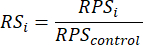
   And the definition of RPM normalization factor (RPM:NF) is same as below:
   
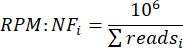
   From here, SRPMC normalization factor (SRPMC:NF) has come out by combining the RS and RPM:NF together:
   
   And this formula can be simplified as below:
   
   Therefore, SRPMC method normalizes reads by the (1) ratio of spike-in reads between control and sample, and (2) RPM normalized control reads. Since this normalization factor considers spike-in reads and makes control reads comparable between samples together, this method would be appropriate to observe genome-wide difference between samples and reduce batch effect in total reads of actual samples and controls in different batch experiments. These normalized bedGraph files will become input files to call peaks using SEACR in section 11. And these normalized bigWig files will be used in loci visualization through IGV and creating heatmap and average plot via Deeptools. It is strongly suggested using a genome browser to visualize the landscape pattern of the CUT&RUN dataset using the normalized bigWig files at representative genomic regions to evaluate data quality. CUT&RUN samples that display noisy background signal patterns that resemble the IgG control are likely appropriate to omit for downstream analyses. Use these shell scripts to normalize other reads bed files and raw readcounts bedGraph files by changing the path and file names for both input and output bed and bedgraph files. Edit these scripts to apply other normalization calculations by changing the factors and formula within this script.

11. Validating fragment size distribution

1. Open the terminal and type echo $SHELL to check the default shell in the active terminal. If Bash shell is the default shell in current terminal, users may see the following: /path/to/bash (or a similar message such as /bin/bash) in the terminal.
2. If the default shell is not Bash, set Bash shell as default shell by typing chsh -s $(which bash) in the terminal. If the terminal uses Bash shell as default, skip this step.
3. Type ~/Desktop/Easy-Shells_CUTnRUN/scripts/Script_10_insert-size-analysis.sh in the terminal or drag the shell script file into the terminal and enter.
   NOTE: This script is written to: (i) Run picard.jar CollectInsertSizeMetrics function using mapped read pairs bam files in ~/Desktop/GSE126612/filtered-bam folder to identify insert size distribution. (ii) Create one folder (~/Desktop/GSE126612/insert-size-distribution) and save the insert size distribution analysis results into the created folder. (iii) Write down a log file per an input bam file in ~/Desktop/GSE126612/log/insert-size-distribution folder.
4. After completion of the run, check the log files carefully. If there is any error message within the log files, correct the error and try to run the shell script again. If there is any problem to solve the issue, request assistance using the Easy Shells CUTnRUN github issues webpage (https://github.com/JunwooLee89/Easy-Shells_CUTnRUN/issues). 
   NOTE: In general, the insert size analysis (Output) for CUT&RUN samples shows major peaks at mono- (100-300 bp) and di- (300-500 bp) nucleosomal size ranges. Technical errors/limitations (such as over-/under-digestion of MNase during CUT&RUN sample preparation or improper size-selection during library preparation) can cause the enrichment of same or larger than tri-nucleosomal (500-700 bp) and same or shorter than sub-nucleosomal (<100 bp) fragments.Sometimes the absence of mono-nucleosomal size peaks with the enrichment of the long (>500 bp) and short fragments (<100 bp) may be due to library size selection ranges chosen at the wet lab stage, or low sequencing depth. Compare sequencing depth ('total sequenced bases' / 'total reference genome size'), genomic landscape overview using normalized readcounts bigWig files in section 10, and the insert size distribution pattern together to clarify the quality of processed CUT&RUN samples. The dashed lines in the histograms represent the 'cumulative fraction' of reads with an insert size greater than or equal to the value on the x-axis. This dashed line enables identification of the distribution of insert sizes in input mapped reads file. Progression along the x-axis is associated with increasing insert size. The dashed line identifies the proportion of mapped read pairs in the input bam file that have an insert size at least as large as indicated on the intersecting x-axis position. Therefore, interpretation begins at 1 on the left, indicating all reads have an insert size greater than or equal to the smallest size, and decreases towards 0 as the insert size increases.

12. Calling peaks using MACS2, MACS3 and SEACR

1. Open the terminal and type echo $SHELL to check the default shell in the active terminal. If Bash shell is the default shell in current terminal, users may see the following: /path/to/bash (or a similar message such as /bin/bash) in the terminal.
2. If the default shell is not Bash, set Bash shell as default shell by typing chsh -s $(which bash) in the terminal. If the terminal uses Bash shell as default, skip this step.
3. Type ~/Desktop/Easy-Shells_CUTnRUN/scripts/Script_11_peak-calling_MACS.sh in the terminal or drag the shell script file into the terminal and enter.
   NOTE: This script is written to: (i) Run macs2 callpeak and macs3 callpeak functions with and without IgG control using fragment BEDPE files to call peaks and save the peak calling results in output directories (~/Desktop/GSE126612/MACS2 and ~/Desktop/GSE126612/MACS3). (ii) Write down the log of these peak callings as text file in log directory (~/Desktop/GSE126612/log/MACS2 and ~/Desktop/GSE126612/log/MACS3)
4. Type ~/Desktop/Easy-Shells_CUTnRUN/scripts/Script_11_peak-calling_SEACR.sh in the terminal or drag the shell script file into the terminal and enter.
   NOTE: This script is written to: (i) Run SEACR_1.3.sh script with and without IgG control, with stringent and relaxed options using raw readcounts bedGraph and normalized bedGraph files to call peaks. (ii) Create output directory (~/Desktop/GSE126612/SEACR-peaks) and save the peak calling results by SEACR. (iii) Write down the log of these peak callings as text file in log directory (~/Desktop/GSE126612/log/SEACR).
5. After completion of running shell scripts, check the log files carefully. If there is any error message in the log files, correct the error first. Some programs may not call peaks for IgG control sample with IgG control option together, thus, omit the error message regarding IgG control sample with IgG control option. If there is any problem to solve the issue, request assistance using the Easy Shells CUTnRUN github issues webpage (https://github.com/JunwooLee89/Easy-Shells_CUTnRUN/issues). 
   NOTE: These two shell scripts perform peak calling for CUT&RUN samples using three peak callers (MACS2, MACS3 and SEACR) with various options: with/without IgG control option, using raw readcounts bedGraph files with normalization option of peak caller or normalized readcounts bedGraph files without normalization option of peak caller, and stringent and relaxed SEACR peak calling options. Since the peak calling output files are not sufficient to be used directly in downstream analyses, Easy Shells CUTnRUN includes one script to process these called peaks output files to create new peak files which includes chromosome, start, end and name of peaks.Through intensive peak calling approaches, Easy Shells CUTnRUN provides an opportunity to choose the peak calling program best suited for a user's CUT&RUN project by comparing the peaks called across three peak callers. In addition, this CUT&RUN analysis pipeline also provides an opportunity to select peak calling options best suited for a user's CUT&RUN project. These comparisons will be done by Venn diagram, and visualization as heatmap and average plot.

13. Creating called peak bed files

1. Open the terminal and type echo $SHELL to check the default shell in the active terminal. If Bash shell is the default shell in current terminal, users may see the following: /path/to/bash (or a similar message such as /bin/bash) in the terminal.
2. If the default shell is not Bash, set Bash shell as default shell by typing chsh -s $(which bash) in the terminal. If the terminal uses Bash shell as default, skip this step.
3. Type ~/Desktop/Easy-Shells_CUTnRUN/scripts/Script_12_make-peak-bed.sh in the terminal or drag the shell script file into the terminal and enter.
   NOTE: This script is written to: (i) Run awk function using bed files in ~/Desktop/GSE126612/SEACR folder to create two types of SEACR peak bed files ~/Desktop/GSE126612/peak-bed_SEACR folder. The whole peak bed files include the start and end of each peak, and the focused peak bed files include the start and bed of highest signal bin within each peak. (ii) Run awk function using ***_peaks.xls files in ~/Desktop/GSE126612/MACS2 and ~/Desktop/GSE126612/MACS3 folders to create whole peak bed files which includes start and end of the each peak called by MACS2 and MACS3 in ~/Desktop/GSE126612/peak-bed_MACS2 and ~/Desktop/GSE126612/peak-bed_MACS3 folders. (iii) Run awk function using ***_summits.bed files in ~/Desktop/GSE126612/MACS2 and ~/Desktop/GSE126612/MACS3 folders to create focused peak bed files which includes start and end of the most significant bin within each peak. (iv) Log files are written in text file format in ~/Desktop/GSE126612/log/peak-bed folder.
4. Type ~/Desktop/Easy-Shells_CUTnRUN/scripts/Script_13_filter-peaks.sh in the terminal or drag the shell script file into the terminal and enter.
   NOTE: This script is written to: (i) Run bedtools intersect function using peak bed files which are called without IgG control option to remove peaks overlapped with IgG control peaks. (ii) The filtered peak bed files are saved in ~/Desktop/GSE126612/peak-bed-filtered_MACS2, ~/Desktop/GSE126612/peak-bed-filtered_MACS3, and ~/Desktop/GSE126612/peak-bed-filtered_SEACR folders. (iii) A log file log_filter-peaks.txt is created in ~/Desktop/GSE126612/log/filter-peaks folder.
5. Type ~/Desktop/Easy-Shells_CUTnRUN/scripts/Script_14_cat-merge-peak-bed_MACS.sh in the terminal or drag the shell script file into the terminal and enter.
   NOTE: This script is written to: (i) Run cat and sort functions to concatenate the replicates' MACS2 and MACS3 whole peak bed files as one peak bed file and sort the concatenated peak bed file in ~/Desktop/GSE126612/bed-for-comparison folder. (ii) Run bedtools merge function using the concatenated whole peak bed files to merge peaks which overlap each other. (iii) A log file log_cat-merged-peak-bed_MACS.txt is written in log folder ~/Desktop/GSE126612/log/cat-merged-peak-bed.
6. Type ~/Desktop/Easy-Shells_CUTnRUN/scripts/Script_14_cat-merge-peak-bed_SEACR.sh in the terminal or drag the shell script file into the terminal and enter.
   NOTE: This script is written to: (i) Run cat and sort functions to concatenate the replicates' SEACR whole peak bed files as one peak bed file and sort the concatenated peak bed file in ~/Desktop/GSE126612/bed-for-comparison folder. (ii) Run bedtools merge function using the concatenated whole peak bed files to merge peaks which overlap each other. (iii) A log file log_cat-merged-peak-bed_SEACR.txt is written in log folder ~/Desktop/GSE126612/log/cat-merged-peak-bed.
7. After completion of the run the shell scripts, review the log files carefully. If there is any error message in the log files, correct the error and run the script(s) again. If there is any problem to solve the issue, request assistance using the Easy Shells CUTnRUN github issues webpage (https://github.com/JunwooLee89/Easy-Shells_CUTnRUN/issues).
   NOTE: The whole peak regions peak bed files will be used as input files of Venn diagram analysis to compare similarity between peak calling options, peak calling methods, replicates, and genomic landscape observations near peak regions. The merged whole peak regions peak bed files will be used for Principal component (PC) analysis and Pearson coefficient correlation analysis using deeptools. The focused peak bed files will be used for Heatmap and average plot analysis using Deeptools.

14. Validating similarity between replicates using Pearson correlation and Principal component (PC) analysis.

1. Open the terminal and type echo $SHELL to check the default shell in the active terminal. If Bash shell is the default shell in current terminal, users may see the following: /path/to/bash (or a similar message such as /bin/bash) in the terminal.
2. If the default shell is not Bash, set Bash shell as default shell by typing chsh -s $(which bash) in the terminal. If the terminal uses Bash shell as default, skip this step.
3. Type ~/Desktop/Easy-Shells_CUTnRUN/scripts/Script_15_correlation_plotCorrelation.sh in the terminal or drag the shell script file into the terminal and enter.
   NOTE: This script is written to: (i) Run multiBamSummary BED-file function using the bam files of replicates, which were sorted by coordinate, and merged whole peak bed files for CTCF, H3K27Ac and RNAPII-S5P to generate matrix files for Pearson correlation analysis in Desktop/GSE126612/deeptools_multiBamSummary folder. (ii) Run plotCorrelation function using the matrix files to perform Pearson correlation coefficient calculation and heatmap clustering and save the result in ~/Desktop/GSE126612/deeptools_plotCorrelation folder. (iii) Write down a log file log_plotCorrelation.txt in ~/Desktop/GSE126612/log/correlation folder.
4. Type ~/Desktop/Easy-Shells_CUTnRUN/scripts/Script_15_correlation_plotPCA.sh in the terminal or drag the shell script file into the terminal and enter.
   NOTE: This script is written to: (i) Run multiBamSummary BED-file function using the bam files, which were sorted by coordinate, and merged whole peak bed files, which includes all the CTCF, H3K27ac and RNAPII-S5P peaks, to generate matrix files for Principal component analysis (PCA) in Desktop/GSE126612/deeptools_multiBamSummary folder. (ii) Run plotPCA function using the matrix files to perform PCA and save the result in ~/Desktop/GSE126612/deeptools_plotPCA folder. (iii) Write down a log file log_plotPCA.txt in ~/Desktop/GSE126612/log/correlation folder.
5. After completion of running shell scripts, check the log files. If there is any error message, correct the error and run the shell scripts again. If there is any problem to solve the issue, request assistance using the Easy Shells CUTnRUN github issues webpage (https://github.com/JunwooLee89/Easy-Shells_CUTnRUN/issues). 
   NOTE: In principle, properly prepared and processed replicates show higher Pearson correlation coefficient values within same clustering group and close positioning in Principal component analysis. Any replicate, which shows a lower Pearson correlation coefficient, and long distance from other replicates in the Principal component plot, may represent a potential outlier among the replicates. This shell script is applicable for any bam format mapped reads data. Change the path and file name of bigwig files to meet project-specific requirements.

15. Validating similarity between replicates, peak calling methods and options using Venn diagram

1. Open the terminal and type echo $SHELL to check the default shell in the active terminal. If Bash shell is the default shell in current terminal, there may be something like /path/to/bash (for example, /bin/bash) in the terminal.
2. If the default shell is not Bash, set Bash shell as default shell by typing chsh -s $(which bash) in the terminal. If the terminal uses Bash shell as default one, consider skipping this step
3. Type ~/Desktop/Easy-Shells_CUTnRUN/scripts/Script_16_venn-diagram_methods.sh in the terminal or drag the shell script file into the terminal and enter.
   NOTE: This script is written to: (i) Run intervene venn function using whole peak region peak bed files to find overlaps between the peaks called by various options (with/without IgG control option, with/without normalization, and stringent/relaxed peak calling options for SEACR). (ii) Create one folder (~/Desktop/GSE126612/intervene_methods) and save the Venn diagram analysis results in this folder. (iii) Write down one log file log_intervene_methods.txt in ~/Desktop/GSE126612/log/intervene folder.
4. Type ~/Desktop/Easy-Shells_CUTnRUN/scripts/Script_16_venn-diagram_replicates.sh in the terminal or drag the shell script file into the terminal and enter.
   NOTE: This script is written to: (i) Run intervene venn function using whole peak region peak bed files to find overlaps between the replicates' peaks. (ii) Create one folder (~/Desktop/GSE126612/intervene_replicates) and save the Venn diagram analysis results in this folder. (iii) Write down one log file log_intervene_replicates.txt in ~/Desktop/GSE126612/log/intervene folder.
5. After the finish of running the shell scripts, review the log files. If there is any error message, correct the error and run the shell scripts again. If there is any issue in usage of Easy Shells CUTnRUN analysis pipeline, ask help in Easy Shells CUTnRUN github issues webpage (https://github.com/JunwooLee89/Easy-Shells_CUTnRUN/issues).
   NOTE: These Venn diagram analysis results give insight to choose the most appropriate peak calling options, methods, and replicates with high reproducibility for downstream analysis. It may be preferred to choose the peak calling options and methods which show the highest called peak numbers with good overlap with other peak calling methods and options.

16. Analyzing heatmaps and average plots to visualize called peaks.

1. Open the terminal and type echo $SHELL to check the default shell in the active terminal. If Bash shell is the default shell in current terminal, there may be something like /path/to/bash (for example, /bin/bash) in the terminal.
2. If the default shell is not Bash, set Bash shell as default shell by typing chsh -s $(which bash) in the terminal. If the terminal uses Bash shell as default one, consider skipping this step
3. Type ~/Desktop/Easy-Shells_CUTnRUN/scripts/Script_27_plotHeatmap_focused.sh in the terminal or drag the shell script file into the terminal and enter.
   NOTE: This script is written to: (i) Run computeMatrix reference-point function using normalized bigWig files and focused peak bed files to make normalized readcounts matrixes at the center of the focused peaks in ~/Desktop/GSE126612/deeptools_computeMatrix folder. (ii) Run plotHeatmap function using the normalized readcounts matrix to generate heatmaps and average plots which visualize normalized readcounts distribution pattern at the focused peak locations. (iii) Create one folder (~/Desktop/GSE126612/deeptools_plotHeatmap) and save the plotHeatmap output files within this folder. (iv) Write down one log file log_plotHeatmap_focused.txt in ~/Desktop/GSE126612/log/plotHeatmap folder.
4. Type ~/Desktop/Easy-Shells_CUTnRUN/scripts/Script_27_plotHeatmap_whole.sh in the terminal or drag the shell script file into the terminal and enter.
   This script is written to: (i) Run computeMatrix reference-point function using normalized bigWig files and whole peak bed files to make normalized readcounts matrixes at the center of the whole peaks in ~/Desktop/GSE126612/deeptools_computeMatrix folder. (ii) Run plotHeatmap function using the normalized readcounts matrix to generate heatmaps and average plots which visualize normalized readcounts distribution pattern at the whole peak locations. (iii) Create one folder (~/Desktop/GSE126612/deeptools_plotHeatmap) and save the plotHeatmap output files within this folder. (iv) Write down one log file log_plotHeatmap_whole.txt in ~/Desktop/GSE126612/log/plotHeatmap folder.
5. After the finish of running the shell scripts, review the log files. If there is any error message, correct the error and run the shell scripts again. If there is any issue in usage of Easy Shells CUTnRUN analysis pipeline, ask help in Easy Shells CUTnRUN github issues webpage (https://github.com/JunwooLee89/Easy-Shells_CUTnRUN/issues).
   NOTE: Ideally, the peak summit locations of MACS2/3 peaks and the focused peak locations of SEACR ones exhibit a sharp and focused signal distribution at the center of the plots. However, if the peak calling algorithm does not work properly for CUT&RUN data, less focused 'noisy' signal distribution may appear in the plots. Therefore, using the number of called peaks and the peak signal distribution patterns of the output plots will guide determination of peak validity for further CUT&RUN analysis that include downstream peak annotation.

Results

Quality and adapter trimming retains reads with high sequencing quality
High-throughput sequencing techniques are prone to generating sequencing errors such as sequence 'mutations' in reads. Furthermore, sequencing adapter dimers can be enriched in sequencing datasets due to poor adapter removal during library preparation. Excessive sequencing errors, such as read mutations, generation of reads shorter than required for proper mapping, and enrichment of adapter dimers, can increase read mapping time and can produce false-positive mapped reads that distort downstream bioinformatic analysis results. Therefore, quality filtering and adapter trimming are required to retain high quality reads for downstream analysis and interpretation.

To retain high quality reads for analysis, this CUT&RUN analysis pipeline (Figure 2) employs FastQC²⁶ and Trim Galore²⁷. The "Script_03_fastQC.sh" shell script runs FastQC for all fastq files within the working directory. Results (Figure 3) of this step using the publicly available CTCF CUT&RUN dataset from GSE126612 (SRR8581589) identify some reads with low-quality score bases (Figure 3A,C) and some degrees of per sequence GC contents distribution mismatch between theoretical estimation and actual reads (Figure 3E).

Execution of the "Script_04_trimming.sh" script to run Trim Galore successfully removes those reads with low-quality score bases (below 20 in Figure 3A) and low mean sequence qualities evident pre-trimming (Figure 3B-D). In addition, "Script_04_trimming.sh" also successfully removes 55~60% mean GC content enrichment displayed in the 'pre-trimming' GC distribution over sequence plot (Figure 3E,F). These results demonstrate that this CUT&RUN analysis pipeline filters for high quality reads to facilitate fast and accurate read mapping to the reference genome.

Insert size distribution can gives estimate for peak calling results
Due to use of MNase in CUT&RUN (Figure 1), mapped CUT&RUN reads are expected to exhibit mono- (~200 bp) and di-nucleosomal (~350 bp) DNA fragment size peaks within insert size distribution plots (Figure 4). Issues with detection for some targets may result in short inserts (< 100 bp) (Figure 4C). High level of short reads reduces the number of reads which can be used for high-confidence peak calling, thus reducing peak numbers and impacting downstream analysis. In this CUT&RUN analysis pipeline, "Script_10_insert-size-analysis.sh" operates "picard.jar CollectInsertSizeMetrics" function to perform the insert size distribution analysis and export histograms as a visualization output (Figure 2). In the output plots (Figure 4A-C), x-axis shows the insert size range, left side of y-axis and filled histogram represents the number of inserts with the value on the x-axis, and right side of y-axis shows and the dashed line the cumulative fraction of inserts with an insert size equal to or greater than the value on the x-axis. Therefore, both the location on the X-axis with the most dramatic change in slope of the dashed line that intersects with the highes level in histogram identifies the major insert size in the sample. Among the reads mapped on reference genome of interest (human, hg19), H3K27Ac (active histone mark) sample fragments exhibit the expected CUT&RUN insert size distribution with highest mono-nucleosomal size and detectable di-nucleosomal size peaks (Figure 4B). CTCF sample fragments showed additional groups at 100~200bp fragment length regions (Figure 4A). Altogether, the CUT&RUN analysis pipeline provides easy-to-use shell scripts to perform insert size distribution analysis after mapping reads on reference genomes. These analyses become important when estimating the efficiency of peak calling before downstream analysis.

Easy Shells CUTnRUN analysis pipeline provides filtrations and normalization options to create trustful readcounts
One of the critical points of CUT&RUN analysis is to obtain proper mapped read pairs by filtering problematic read pairs from the initial mapping outputs and normalizing the filtered mapped readcounts with specific normalization calculation method which can meet the objectives/needs of user's analysis. The CUT&RUN analysis pipeline discussed in this study includes "Script_07_filter-sort-bam.sh" script to remove read pairs which are mapped on either non-canonical chromosomes, publicly annotated blacklist regions²³, and TA repeats regions^18,22 from read pairs which were mapped by bowtie2 using "Script_06_bowtie2-mapping.sh". These filtrations are required to remove read pairs which can produce false-positive, outlier spike signals and called peaks in downstream analysis (Figure 5; yellow box regions).

In addition to the filtrations, applying the correct normalization method is an important factor to visualize the signal difference between samples accurately. Therefore, the CUT&RUN analysis pipeline includes "Script_09_normalization_SFRC.sh" and "Script_09_normalization_SRPMC.sh" scripts to provide two publicly verified normalization methods - the scaled fractional readcout (SFRC)²² and Spike-in normalized Reads Per Million mapped reads in the negative Control (SRPMC)^24,25 (Figure 5A-D). Since SFRC does not include control (for example, IgG) nor spike-in sample in formula, SFRC normalization can be used for samples which do not include any control sample or are expected to show signal differences at local regions only without genome-wide scale difference. The SFRC normalized samples processed by the CUT&RUN analysis pipeline (Figure 5A-D; red tracks) produces the same signal distribution patterns as publicly available mapped reads from GEO (Figure 5A-D; black tracks), suggesting that this pipeline can reproduce the publication results.

The SRPMC method is useful to normalize samples which include both control and Spike-in samples and are expected to show global signal difference between samples (Figure 5A-D; green tracks). Since one H3K27Ac sample (SRR8581599) exhibits much higher "(actual CUT&RUN reads)/(spike-in reads)" ratio (sample RPS; 997) than other replicates (237, 175, and 161), relative H3K27Ac signals appear different between replicates in SFRC and SRPMC normalized samples (Figure 5A-D; H3K27Ac compared across all tracks). RNAPII-S5P samples exhibit relatively lower sample RPS (1.7, 0.8, 2.1) than IgG control (259), thus RNAPII-S5P samples exhibit lower signal than IgG control after SRPMC normalization (Figure 5A-D; RNAPII-S5P compared across all tracks). Therefore, the CUT&RUN analysis pipeline discussed here recommends to use SRPMC method only for the samples which have enough reads in experimental samples relative to both IgG control and spike-in control reads.

Venn diagram comparison can give ideas to choose better peak calling method and options
Multiple peak calling programs enable identification of significantly enriched protein occupancy across genome. Such programs employed for CUT&RUN analysis include MACS family programs² and SEACR⁴ as major methods so far. However, it can be challenging, especially for bioinformatics beginners, to identify the most appropriate peak calling method and options for a given CUT&RUN project. Therefore, the CUT&RUN analysis pipeline includes Venn diagram analysis steps to give a chance for users to compare similarity and difference of the peak calling results between various peak calling options (Script_17_intervene-options), and peak calling programs (Script_19_intervene_methods.sh) (Figure 6A-H).

According to comparison the merged CTCF, H3K27ac, and RNAPII-S5P peaks which are called with and without IgG control option during peak calling step, MACS2 and MACS3 called more peaks with IgG control option (Figure 6A), but SEACR called more peaks without IgG control option in both stringent and relaxed options (Figure 6B-D). Therefore, the CUT&RUN analysis pipeline suggests (1) applying the IgG control option for MACS2 and MACS3, (2) calling peaks for experimental CUT&RUN samples and IgG control samples separately, then filtering out IgG peaks later for the SEACR peak caller. Between MACS2 and MACS3, MACS3 called slightly more peaks (Figure 6A).

Furthermore, comparison of peaks called by MACS2 and MACS3 with IgG control option and SEACR without IgG control option shows that SEACR peaks called with the stringent option overlap with MACS 2 and MACS3 peaks more so than SEACR peaks called with the relaxed option (Figure 6E,F). Thus, the CUT&RUN analysis pipeline outputs suggest that the stringent option maximizes SEACR consistency with MACS peak calling. Finally, the Venn diagram to compare the overlap of peaks called by SEACR with normalization for raw readcounts CUT&RUN bedGraph files and without normalization for normalized readcounts CUT&RUN bedGraph files reveals no difference between SFRC and SRPMC methods for SEACR with the stringent option. SFRC peaks exhibit much higher peak numbers and better overlap with normalized option peaks ('norm' in Figure 6) than SRPMC peaks for SEACR with relaxed options (Figure 6G,H).

Statistical comparisons between replicates and samples
Drawing accurate conclusions across multiple replicates requires an assessment of replicate similarity. The CUT&RUN analysis pipeline used here employs Deeptools2¹⁵ based statistical correlation coefficient calculation, heatmap clustering and principal component analysis (PCA) to facilitate identification of samples and replicates appropriate for valid downstream analysis. The Pearson correlation coefficient based heatmap clustering showed statistically significant correlation between replicates for CTCF, H3K27Ac and RNAPII-S5P at their called peak regions (Figure 7A-C). However, PCA showed that one sample of CTCF (SRR8581590) and H3K27Ac (SRR8581608) are located relatively far from other replicates (Figure 7D) at the all the CTCF, H3K27Ac and RNAPII-S5P called peak regions.

According to the Venn diagram to compare between peaks between replicates, the CTCF (SRR8581590) peaks showed least overlap with other replicates in all three peak caller results (Figure 7E-G), and H3K27Ac (SRR8581608) peaks showed least overlap with other replicates in SEACR peak calling results (Figure 7F). the H3K27Ac (SRR8581608) peaks did not exhibit minimum overlap with other replicates in MACS2 and MACS3 peak calling results (Figure 7F), which may suggest that the distance between replicates in PCA is not sufficient to define outlier sample. Therefore, the CUT&RUN analysis pipeline proposes to define outlier replicate as 'the sample which shows low Pearson correlation coefficient in heatmap clustering group, long distance in PCA plot with other replicates, and lowest peak overlap across replicates'.

Peak calling facilitates visualization and interpretation of CUT&RUN data
The CUT&RUN analysis pipeline detailed in this study employs two types of publicly available peak callers: MACS family and SEACR. To optimize the visualization of called peaks, this pipeline selects the highest signal bin as the peak center for heatmap and metaplot analyses. All the CTCF, H3K27Ac and RNAPII-S5P peaks called by MACS3 and SEACR peak callers showed more sharp peak distribution pattern at the center of highest signal bins (Figure 8A-F, 'focused' plots) than the center of whole peak regions (Figure 8A-F, 'whole' plots). CUT&RUN samples processed by Easy Shells CUTnRUN analysis pipeline with SFRC normalization (Figure 8 A-F, 'SFRC' plots) exhibit similar signal distribution patterns with that of the SFRC normalized samples of which raw mapped read pairs are publicly available in GEO (Figure 8A-F, 'public' plots) at the peaks called by the analysis pipeline. Thus, the CUT&RUN analysis pipeline can reproduce publication results successfully.

Figure 1: Schematic of CUT&RUN experimental procedure. CUT&RUN is an enzyme-based approach to detect protein-DNA interactions across the genome. The CUT&RUN procedure begins with binding of cells (or isolated nuclei) to Concanavalin A conjugated to magnetic beads to enable isolation and manipulation of low cell numbers throughout the procedure. Isolated cells are permeabilized using a mild detergent to facilitate introduction of an antibody that targets the protein of interest. Micrococcal nuclease (MNase) tethered to Protein A or Protein A/G tag is then introduced into the permeabilized cell. pA-MNase (or pAG-MNase) is recruited to the bound antibody using a Protein A or Protein A/G tag. Once MNase is localized to the target sites, the nuclease is briefly activated through introduction of calcium to digest the DNA around the target protein. MNase digestion results in mono-nucleosomal DNA-protein complexes. Calcium is subsequently chelated to end the digestion reaction, and short DNA fragments from the MNase digestion are released from nuclei by a short incubation at 37°C, then subjected to DNA purification, library preparation, and high-throughput sequencing¹. Please click here to view a larger version of this figure.

Figure 2: Schematic summary of Easy-Shell CUT&RUN analysis pipeline. The Easy-Shell CUT&RUN analysis pipeline is designed in three major sections - (1) quality control and mapping of raw read files (left; purple), (2) normalization of mapped reads and readcounts and peak calling (center; green), and (3) validation of mapped reads and called peaks (right; pink). In each step, the corresponding shell script number, a brief description, and the program tool used in that step (in brackets) are provided. Plaine arrows show direct flows between steps. This CUT&RUN analysis pipeline provides two read normalization methods which can meet the needs of users with and without control reads, multi-layer validation processes to identify proper replicates for downstream analysis, and focused peak identification for well-focused heatmap and metaplot output creation. This analysis pipeline is written in easy-to-use shells scripts in a step-by-step manner to provide bioinformatics beginners the opportunity to learn and practice basic CUT&RUN data analysis by reading and editing the scripts themselves. Please click here to view a larger version of this figure.

Figure 3: Comparison of quality check results pre- versus post quality trimming. Select quality check report outputs from FastQC display the effect of quality trimming using reads from SRR8581589 (GSM3609748, CTCF). Outputs shown include: (A) Quality score across bases pre-trimming. (B) Same readout as A) post-trimming. (C) Quality score distribution over all sequences pre-trimming. (D) Same readout as C) post-trimming. (E) GC distribution over all sequences pre-trimming. (F) Same readout as E) post-trimming. The minimum quality score at each position within sequencing reads (A, B) and minimum mean sequence quality (C, D) are increased after quality trimming. Furthermore, this step can reduce the difference between theoretical GC counts distribution and actual GC count per base in the reads (E, F) by removing reads pairs which have high base mismatch ratio. Please click here to view a larger version of this figure.

Figure 4: Insert size distribution analysis. Insert size histogram for (A) CTCF, (B) H3K27Ac, and (C) serine 5 phosphorylated RNA polymerase II (RNAPII-S5P). Histograms display relative differences in insert size distribution between samples. The dashed line in the histogram represents the cumulative fraction of reads with an insert size greater than or equal to the value on the x-axis. n: number of concordantly mapped unique reads per sample after filtration. FR: fragments. Please click here to view a larger version of this figure.

Figure 5: Landscape overview of the CUT&RUN samples. Publicly available CUT&RUN mapped reads normalized by the scaled fractional count (SFRC) without additional filtration (black tracks), the CUT&RUN samples processed by Easy Shells CUTnRUN analysis pipeline with SFRC normalization (red tracks) and 'Spike-in normalized Reads Per Million mapped reads in the negative Control (SRPMC; green tracks)' are shown at (A) histone genes cluster region, and (B-D) other three regions with CTCF, H3K27Ac and RNAPII-S5P peaks called by all of MACS2, MACS3 and SEACR peak callers. Yellow boxes highlight the location of spike signals filtered out during the filtration step in Easy Shells CUTnRUN analysis pipeline. Please click here to view a larger version of this figure.

Figure 6: Venn diagram to compare between peaks called by different peak callers and peak calling options. (A) Comparison between peaks called by MACS2 and MACS3 with and without IgG input option during peak calling. (B-D) Comparison between peaks called by SEACR with and without IgG input option, 'stringent' and 'relaxed' options, and with normalization option using raw read pairs files (B), without normalization option using SFRC normalized readcounts files (C) or SRPMC normalized readcounts files (D). (E,F) Comparison between peaks called by MACS2, MACS3 with IgG input option and SEACR with stringent (E) or relaxed (F) option. (G,H) Comparison between peaks called by SEACR without IgG input option and with stringent (G) or relaxed (H) options. w/ IgG: peaks called with IgG input option. w/o IgG: peaks called without IgG input option. norm: peaks called with normalization option. non: peaks called without normalization option. SFRC: peaks called by readcounts files normalized by the 'scaled fractional count (SFRC)' method. SRPMC: peaks called by readcounts files normalized by the 'Spike-in normalized Reads Per Million mapped reads in the negative Control (SRPMC) method'. Please click here to view a larger version of this figure.

Figure 7: Pearson correlation, Principal component analysis and Venn diagram to validate the similarity between replicates. (A-C) Heatmap clustering with Pearson correlation coefficient values display the degree of similarity between replicates at the peaks called by MACS2 (A), MACS3 (B) and SEACR (C). Pearson correlation coefficient is in a value between -1 and 1. A larger absolute Pearson correlation coefficient value indicates a stronger correlation between two variables, and a positive Pearson correlation coefficient value indicates a positive correlation, where the two variables move in the same direction. Therefore, samples with higher similarity exhibit closer pedigree in Heatmap clustering and higher Pearson coefficient value. (D) Principal component analysis (PCA) displays degree of similarity between replicates and samples at all the CTCF, H3K27Ac and RNAPII-S5P peak regions which are called by MACS2 (left), MACS3 (center) and SEACR (right). Samples with higher similarity are positioned closer together in the PCA plot. (E-G) Venn diagram analysis to compare the peaks found in each replicate by MACS2 (E), MACS3 (F), and SEACR (G). Easy-Shell CUT&RUN analysis pipeline proposed to apply all of three methods to identify replicates with high similarity that may be suitable to merge the called peaks for downstream analysis. Please click here to view a larger version of this figure.

Figure 8: Heatmap and metaplot visualization of signal distribution at peaks. Heatmap and metaplots display distribution of enrichment around peak centers called using different peak callers. (A,B) CTCF CUT&RUN peaks called from one replicate (SRR8581589) by MACS3 (A) and SEACR (B). (C,D) H3K27Ac CUT&RUN peaks called from one replicate (SRR8581607) using MACS3 (C) and SEACR (D). (E,F) RNAPII CUT&RUN peaks called from one replicate (SRR8581589) by MACS3 (E) and SEACR (F). Publicly available mapped read pairs ('Public' in Figure 8) and the fragments mapped by Easy Shells CUTnRUN analysis pipeline ('SFRC' in Figure 8) are compared after 'scaled fractional count (SFRC)' normalization. Peaks are called by MACS3 with IgG input option ('MACS3 w/ IgG' in Figure 8) and SEACR without IgG input and without normalization option using SFRC normalized readcounts files in stringent mode ('SEACR w/o IgG non SFRC stringent' in Figure 8). Two versions of coordinate files of the called peaks are prepared: from the start to the end of the called peaks ('whole' in Figure 8) and the location of bin with highest signal within the called peaks (summits in MACS3 called peaks; 'focused' in Figure 8). Please click here to view a larger version of this figure.

Table 1: Information for CUT&RUN fastq files in GSE126612. All the raw reads CUT&RUN fastq files which are included in GSE126612 and are selected as example dataset for Easy Shells CUTnRUN analysis pipeline are listed as a table. The 'File Name' column shows file names of raw CUT&RUN reads fastq files which will be shown in '~/Desktop/GSE126612/fastq' after running 'Script_02_download-fastq.sh'. 'md5sum' shares MD5 (Message-Digest Algorithm 5) for the example dataset which can be used to verify the integrity of files after downloading the dataset via running 'Script_02_download-fastq.sh'. The last column describes target of CUT&RUN per each sample. Please click here to download this Table.

Discussion

The ability to map protein occupancy on chromatin is fundamental to conducting mechanistic studies in the field of chromatin biology. As laboratories adopt new wet lab techniques to profile chromatin, the ability to analyze sequencing data from those wet lab experiments becomes a common bottleneck for wet lab scientists. Therefore, we describe an introductory step-by-step protocol to enable bioinformatics beginners to overcome the analysis bottleneck, and initiate analysis and quality control checks of their own CUT&RUN sequencing data.

This CUT&RUN analysis protocol describes the application of several steps to ensure bona fide signals are quantified. The removal of poor-quality reads and adapter sequences from raw read data is one of the first quality control steps, and one of the most critical steps to obtain accurate analysis outcomes. Therefore, this analysis pipeline includes easy-to-apply quality and adapter trimming steps using the Trim-galore program²⁷. Due to the importance of this process, this analysis pipeline includes steps to compare the quality of results before (step 4.3) and after (step 5.3) the trimming process (step 5.5). In addition to quality and adapter trimming, this analysis pipeline also removes non-canonical chromosome reads, TA repeat regions, and blacklist regions, which can introduce GC content bias and false-positive spikes/called peaks. These filtration steps provide an appropriate introductory pipeline for bioinformatics beginners to understand the critical quality control steps for CUT&RUN data analysis.

After the filtration step, this CUT&RUN analysis pipeline provides two normalization options: 'scaled fractional readcount (SFRC)²²' and 'Spike-in normalized Reads Per Million mapped reads in the negative Control (SRPMC)^24,25 to create input files for downstream peak calling and visualization. If CUT&RUN dataset is expected to reveal local differences only without genome-wide signal differences between samples, the scaled fractional readcount (the fraction of counts times the size of reference gnome) may suffice for downstream analysis. However, if there is possibility that global scale signal differences will be present between CUT&RUN samples, users can choose the SRPMC method that considers the ratio of reads between spike-in and sample (both experimental CUT&RUN and negative control samples) along with reads per million (RPM) normalization for negative control reads to make the negative control reads comparable between different samples. Since the SRPMC provides normalized reads relative to normalized negative control reads, this approach minimizes the negative control signal enables comparison between datasets created in different batches and groups.

An important factor in CUT&RUN sample peak calling is eliminating false positive CUT&RUN peaks during the in silico analysis, in part, through inclusion of IgG samples. Specifically, this analysis pipeline provides peak calling approaches for different peak callers to discard false positive CUT&RUN called peaks. For MACS2/3 peak callers, our analysis pipeline applies IgG mock reads as input sample during peak calling. For SEACR, this analysis pipeline recommends calling the peaks for experimental samples and negative control samples independently first, and then removing the peaks that overlap between experimental samples and negative control samples since SEACR may 'lose' a majority of peaks if provided with the negative control during the peak calling of the experimental samples. Curated peaks exhibit comparable similarity between different peak callers and replicates (Figure 5). Altogether, removal of poor quality, non-canonical chromosomes, blacklist region, and TA repeats reads, adapter sequences trimming, spike-in DNA normalization, and proper handling of negative control during peak calling steps provides users with proper readcounts files that are suitable for downstream analyses. With high-quality normalized read files and curated called peaks, users can proceed to compare similarity between replicates and create heatmaps and metaplots with ultra-clean background signal to validate the effective peak calling.

Peak calling with high-quality reads marks the initiation of drawing biological interpretations from CUT&RUN data. This protocol describes obtaining focused peak signals in heatmaps and metaplots by appointing the highest signal or most statistically significant signal locations as peak centers. Some peak calling approaches do not select the highest signals or most statistically significant signals at their center location. Therefore, re-defining the center of each peak as the highest signal or most statistically significant signal location serves as an important step to create visual data outputs with well-focused signals at the center of the plots. Bed files of original called peaks are retained to perform peak annotation and functional relevance analysis as next steps after completion of the steps described in this protocol.

Although this CUT&RUN analysis pipeline includes steps to describe installation of required programs, beginners in bioinformatics may encounter difficulties in installing the analysis tools. Therefore, an associated Github issue page has been established to provide more detailed step-by-step descriptions for program installation and to facilitate communications to support users during program installation in their own system. Next steps in the CUT&RUN analysis pipeline beyond the protocol described in this article include peak annotation, identifying overlaps between different types of called peaks, and functional annotation for called peaks. Completion of quality control steps and peak calling described in this protocol combined with downstream peak annotation will enable users to draw biological meaning from their CUT&RUN data.

This CUT&RUN analysis pipeline has been built to provide general introductory step-by-step guidelines for bulk CUT&RUN analysis. This pipeline possesses some limitations. First, although this analysis pipeline is trying to handle GC contents variation driven effect by filtering out reads on blacklist regions (which include "high signal artifact regions" and "artifact repeat regions", and TA repeat regions) this approach may not be sufficient for some organisms that may have distinctive GC content on their genome. Therefore, if users are concerned of any GC content-driven biases, consider adding another step to correct mapped reads. For bioinformatics beginners, 'computeGCBias' and 'correctGCBias' in Deeptools may be options for this objective. Second, this analysis pipeline is handling both regular insert size (100 bp-1 kb) and small insert size reads (< 100 bp), which may be the actual reads of some chromatin-associated proteins, within same file. Since this analysis pipeline is written in shell scripts, users can modify "Script_08_bam-to-BEDPE-BED-bedGraph.sh" to grab the short insert size reads separately from regular fragment size reads during the mapped reads bed file generation step. Subsequently, the short insert size reads bed file can be normalized independently from regular insert size mapped reads to minimize the downsizing effect. Third, to reduce the complexity of analysis pipeline, Easy Shells CUTnRUN does not include a down-sampling step to match the sequencing depth of CUT&RUN samples. However, users can apply a down-sample step after filtering bam files by using samtools view²⁸ or PositionBasedDownsampleSam (Picard)²⁹.

All the analysis steps in this protocol are written in shell scripts to enable bioinformatics beginners to learn the basics of CUT&RUN analysis by reviewing the scripts. We expect that users can practice bioinformatics analysis in a step-by-step manner by running each shell script sequentially in the terminal. Furthermore, the simplicity of the shell scripts provided in this CUT&RUN analysis pipeline allows users to revise and customize these scripts to apply this analysis pipeline to their own CUT&RUN data. Ultimately, we expect that this CUT&RUN analysis pipeline can reduce common bottlenecks in the CUT&RUN data analysis process to empower wet lab researchers and bioinformatics beginners to draw biological conclusions from their own CUT&RUN sequencing data.

Materials

List of materials used in this article

Name	Company	Catalog Number	Comments
bedGraphToBigWig	ENCODE	https://hgdownload.soe.ucsc.edu/admin/exe/	Software to compress and convert readcounts bedGraph to bigWig
bedtools-2.31.1	The Quinlan Lab @ the U. of Utah	https://bedtools.readthedocs.io/en/latest/index.html	Software to process bam/bed/bedGraph files
bowtie2 2.5.4	Johns Hopkins University	https://bowtie-bio.sourceforge.net/bowtie2/index.shtml	Software to build bowtie index and perform alignment
CollectInsertSizeMetrics (Picard)	Broad institute	https://github.com/broadinstitute/picard	Software to perform insert size distribution analysis
Cutadapt	NBIS	https://cutadapt.readthedocs.io/en/stable/index.html	Software to perform adapter trimming
Deeptoolsv3.5.1	Max Planck Institute	https://deeptools.readthedocs.io/en/develop/index.html	Software to perform Pearson coefficient correlation analysis, Principal component analysis, and Heatmap/average plot analysis
FastQC Version 0.12.0	Babraham Bioinformatics	https://github.com/s-andrews/FastQC	Software to check quality of fastq file
Intervenev0.6.1	Computational Biology & Gene regulation - Mathelier group	https://intervene.readthedocs.io/en/latest/index.html	Software to perform venn diagram analysis using peak files
MACSv2.2.9.1	Chan Zuckerberg initiative	https://github.com/macs3-project/MACS/tree/macs_v2	Software to call peaks
MACSv3.0.2	Chan Zuckerberg initiative	https://github.com/macs3-project/MACS/tree/master	Software to call peaks
Samtools-1.21	Wellcome Sanger Institute	https://github.com/samtools/samtools	Software to process sam/bam files
SEACRv1.3	Howard Hughes Medial institute	https://github.com/FredHutch/SEACR	Software to call peaks
SRA Toolkit Release 3.1.1	NCBI	https://github.com/ncbi/sra-tools	Software to download SRR from GEO
Trim_Galore v0.6.10	Babraham Bioinformatics	https://github.com/FelixKrueger/TrimGalore	Software to perform quality and atapter trimming

References

- Hainer, S. J., Fazzio, T. G. High-resolution chromatin profiling using CUT&RUN. Curr Protoc Mol Biol. 126 (1), e85(2019).
- Zhang, Y., et al. Model-based analysis of ChiP-Seq (MACS). Genome Biology. 9 (9), R137(2008).
- Xu, S., Grullon, S., Ge, K., Peng, W. Stem cell transcriptional networks: Methods and Protocols. , Springer. New York, NY. (2014).
- Meers, M. P., Tenenbaum, D., Henikoff, S. Peak calling by sparse enrichment analysis for cut&run chromatin profiling. Epigenetics Chromatin. 12 (1), 42(2019).
- Ashburner, M., et al. Gene ontology: Tool for the unification of biology. The gene ontology consortium. Nat Genet. 25 (1), 25-29 (2000).
- Harris, M. A., et al. The gene ontology (GO) database and informatics resource. Nucleic Acids Res. 32 (Database issue), D258-D261 (2004).
- The Gene Ontology Consortium. The gene ontology resource: 20 years and still going strong. Nucleic Acids Res. 47 (D1), D330-D338 (2019).
- Conesa, A., et al. Blast2go: A universal tool for annotation, visualization and analysis in functional genomics research. Bioinformatics. 21 (18), 3674-3676 (2005).
- Carbon, S., et al. AmiGO: Online access to ontology and annotation data. Bioinformatics. 25 (2), 288-289 (2009).
- Eden, E., Navon, R., Steinfeld, I., Lipson, D., Yakhini, Z. Gorilla: A tool for discovery and visualization of enriched go terms in ranked gene lists. BMC Bioinformatics. 10, 48(2009).
- Huang Da, W., Sherman, B. T., Lempicki, R. A. Bioinformatics enrichment tools: Paths toward the comprehensive functional analysis of large gene lists. Nucleic Acids Res. 37 (1), 1-13 (2009).
- Huang Da, W., Sherman, B. T., Lempicki, R. A. Systematic and integrative analysis of large gene lists using david bioinformatics resources. Nat Protoc. 4 (1), 44-57 (2009).
- Ge, S. X., Jung, D., Yao, R. ShinyGO: A graphical gene-set enrichment tool for animals and plants. Bioinformatics. 36 (8), 2628-2629 (2020).
- Tang, D., et al. SRplot: A free online platform for data visualization and graphing. PLoS One. 18 (11), e0294236(2023).
- Ramírez, F., et al. Deeptools2: A next generation web server for deep-sequencing data analysis. Nucleic Acids Res. 44 (W1), W160-W165 (2016).
- Robinson, J. T., et al. Integrative genomics viewer. Nat Biotechnol. 29 (1), 24-26 (2011).
- Kent, W. J., et al. The human genome browser at ucsc. Genome Res. 12 (6), 996-1006 (2002).
- Yu, F., Sankaran, V. G., Yuan, G. -C. CUT&RUNTools 2.0: A pipeline for single-cell and bulk-level CUT&RUN and CUT&Tag data analysis. Bioinformatics. 38 (1), 252-254 (2021).
- Zhu, Q., Liu, N., Orkin, S. H., Yuan, G. -C. CUT&RUNTools: A flexible pipeline for CUT&RUN processing and footprint analysis. Genome Biol. 20 (1), 192(2019).
- Chris Cheshire, C. -W., et al. Nf-core/cutandrun: Nf-core/cutandrun v3.2.2 iridium ibis. , At https://github.com/nf-core/cutandrun/tree/3.2.2 (2024).
- Kong, N. R., Chai, L., Tenen, D. G., Bassal, M. A. A modified CUT&RUN protocol and analysis pipeline to identify transcription factor binding sites in human cell lines. STAR Protoc. 2 (3), 100750(2021).
- Meers, M. P., Bryson, T. D., Henikoff, J. G., Henikoff, S. Improved CUT&RUN chromatin profiling tools. eLife. 8, e46314(2019).
- Amemiya, H. M., Kundaje, A., Boyle, A. P. The encode blacklist: Identification of problematic regions of the genome. Sci Rep. 9 (1), 9354(2019).
- Deberardine, M. BRgenomics for analyzing high-resolution genomics data in R. Bioinformatics. 39 (6), btad331(2023).
- Deberardine, M., Booth, G. T., Versluis, P. P., Lis, J. T. The nelf pausing checkpoint mediates the functional divergence of cdk9. Nat Commun. 14 (1), 2762(2023).
- Andrews, S. Fastqc: A quality control tool for high throughput sequence data. , At http://www.bioinformatics.babraham.ac.uk/projects/fastqc/ (2010).
- Krueger, F., James, F. O., Ewels, P. A., Afyounian, E., Schuster-Boeckler, B. FelixKrueger/TrimGalore: v0.6.7 - DOI via Zenodo. , (2021).
- Mcgaughey, D. Easy bam downsampling. , Available from: https://davemcg.github.io/post/easy-bam-downsampling/ (2018).
- Positionbaseddownsamplesam (picard). , GATK Team. At https://gatk.broadinstitute.org/hc/en-us/articles/360041850311-PositionBasedDownsampleSam-Picard (2020).
Access restricted. Please log in or start a trial to view this content.
Reprints and Permissions