We present development of a gaze-contingent display framework designed for perceptual and oculomotor research simulating central vision loss. This framework is particularly adaptable for studying compensatory behavioral and oculomotor strategies in individuals experiencing both simulated and pathological central vision loss.
A subscription to JoVE is required to view this content. Sign in or start your free trial.
Method Article
A Gaze-Contingent Display Framework for Perceptual Learning Research with Simulated Central Vision Loss
* These authors contributed equally
In This Article
Summary
Abstract
Macular degeneration (MD) is one of the leading causes of vision impairment in the Western world. Patients with MD tend to develop spontaneous eye movement strategies to compensate for their vision loss, including adopting a preferred retinal locus, or PRL, a spared peripheral region that they use more frequently to replace the damaged fovea. However, not all patients are successful in developing a PRL, and even when they do, it might take them months. Currently, no gold standard rehabilitative therapy exists, and MD research is further hindered by issues of recruitment, compliance, and comorbidity. To help address these issues, a growing body of research has used eye tracking-guided, gaze-contingent displays in a simulated central vision loss paradigm in individuals with intact vision. While simulated vision loss is qualitatively different than pathological central vision loss, our framework provides for a highly controlled model through which to study compensatory eye movements and test possible rehabilitation interventions in low vision. By developing a comprehensive framework, rather than relying on isolated and disconnected tasks, we create a cohesive environment where we can test larger-scale hypotheses, allowing us to examine interactions between tasks, assess training effects across multiple measures, and establish a consistent methodology for future research. Furthermore, participants in simulated central vision loss studies show similarities in their oculomotor compensatory behaviors compared to patients with MD. Here, we present a framework for conducting gaze-contingent studies related to simulated central vision loss. We emphasize the utilization of the framework to test behavioral and oculomotor performance of healthy individuals on a wide range of perceptual tasks encompassing different levels of visual processing. We also discuss how this framework can be adapted for training MD patients.
Introduction
Macular degeneration (MD) is the main cause of vision impairment globally, and it is projected to affect 248 million people worldwide by 20401. Late-stage MD is characterized by damage to the photoreceptors in the center of the visual field (fovea). Loss of central vision has severe effects on daily tasks that rely on central vision, such as navigation2, reading3, and recognizing faces4. Consequences of MD greatly impact the quality of life of these individuals5 and lead to negative psychological consequences6. Patients with MD, deprived of their central vision, may spontaneously develop compensatory oculomotor strategies involving the use of a peripheral retinal region to replace the fovea (Figure 1). This region, referred to as the preferred retinal locus (PRL)7, is often adopted by patients in tasks involving fixation, reading, and face recognition. There is evidence of the PRL, in patients with MD, taking over oculomotor referencing duties of the fovea8,9. Further, changes in attention and cognitive control are observed in patients with central vision loss, suggesting a relationship between vision loss and cognitive functions10.

Figure 1. Illustration of the perceptual experience of individuals with healthy vision and macular degeneration patients with foveal scotoma. Foveal scotoma leads to central vision loss in patients with macular degeneration. Some individuals can partially compensate for the loss of visual input to the fovea by using a peripheral retinal location, defined as preferred retinal locus (PRL). In patients that developed a PRL, this is often used for eccentric fixation and during daily tasks. Retinal location, shape and size of the PRL can vary from person to person. Please click here to view a larger version of this figure.
While no gold standard intervention exists to recover vision loss or to compensate for loss of central vision, experimental approaches from optometry, occupational therapy and vision science are being tested to improve compensation through peripheral vision11,12. Oculomotor approaches focus on teaching patients to improve eye movement control and coordination, including teaching them to use a more adequate PRL11,12,13,14,15 while perceptual interventions focus on improving the general peripheral visual abilities or vision within the PRL, partially overcoming the limitation of peripheral vision16,17,18,19,20. Recent studies have used an eye-tracking based gaze-contingent display as a paradigm for the study of eye movements in central vision loss21,22,23,24,25,26,27,28,29. This approach, which utilizes a simulated scotoma (i.e., an occluder to obstruct the central region of the visual field) in healthy individuals (Figure 1), mitigates issues of recruitment and compliance, while providing high control on several parameters, such as the size and shape of the scotoma, thereby offering a promising alternative to the direct involvement of patients with MD. While there exists several differences between central vision loss and simulated scotoma30,31, some of the oculomotor behavior observed in the former, such as the development of a PRL, can be seen in the latter27,30,32, suggesting that some aspects of compensatory oculomotor strategies can be elicited by this gaze-contingent paradigm. Importantly, simulated central vision loss provides a broad framework for studying plasticity in both the healthy visual system and following central vision loss.
Here, we present the design, development, and use of a gaze-contingent framework that can be used to test perceptual, oculomotor, and attentional performances in healthy individuals and, with some modifications, in MD patients (Figure 2). We also detail the technical and psychophysical considerations that accompany gaze-contingent, peripheral training. A key technical challenge involves creating the perception of a smooth, short latency movement of the scotoma33. This short latency is obtained by selecting appropriate display devices, eye trackers, and operating systems34,35,36. Previous work has documented how each piece of hardware adds latency37 and strategies to reduce overall latency, accommodate blinks, and slow eye movements33. A novel aspect of our paradigm is the diverse set of training and assessment tasks within a single framework for perceptual research in both healthy and patient populations. The framework characterizes multiple levels of visual processing affected by central vision loss, specifically low-level vision, higher-level vision, attention, oculomotor control, and cognitive control. Preliminary tests conducted using a modified version of this approach showed evidence of improvement in visual acuity in both healthy controls and the patient population32.
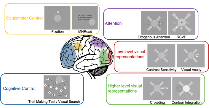
Figure 2. Multidimensional approach to the study of plasticity in the visual system, and vision rehabilitation in Macular Degeneration. Illustration of interconnected dimensions such as visual perception, oculomotor, and cognitive control that contribute to visual processing and are affected in central vision loss. Please click here to view a larger version of this figure.
Access restricted. Please log in or start a trial to view this content.
Protocol
All participants were healthy individuals with visual acuity of 20/40 or above and no known vision issues. Both the representative participants are females, and their ages are 27 and 24. All participants provided informed consent, and the study received approval from the Institutional Review Board (IRB) at the University of Alabama at Birmingham.
1. Identifying an ideal system for simulated central vision loss research
- Identify a system that efficiently transmits information from the eye tracker to the stimulus generation software in a continuous loop. Use methods described in37 to measure the latency of different combinations of systems to identify the one with the lowest latency.
NOTE: A comparison of the combined latency of four different combinations of systems comprising two eye trackers (EyeLink 1000 Plus Tower Mount and TRACKPixx3), two display devices (CRT Monitor (refresh rate = 100Hz) and Display++ (refresh rate = 120Hz)) along with two operating systems (Windows 10 and Mac iOS) is shown in Figure 3. Each combination was measured 20 times. Results showed that system latency was the lowest when Vpixx TrackPixx3 eye tracker was used in combination with the Windows 10 operating system.
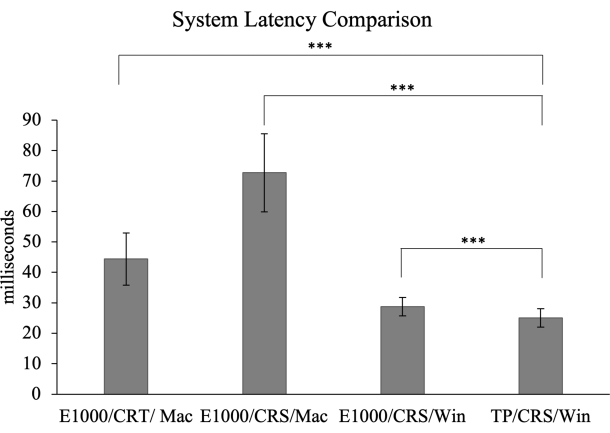
Figure 3: Latency comparison across different combinations of monitors, eye-tracking devices, and operating systems. Bars represent the ± 1 standard deviation across the 20 repetitions per combination. Measures were taken with a Mac operating system phone in slow motion mode, reaching a refresh rate of 240Hz. TP/CRS/Win is statistically different from E1000/CRT/Mac (t(38)=9.53, p<0.001), E1000/CRS/Mac (t(38)=16.24, p<0.001) and E1000/CRS/Win (t(38)=3.94, p<0.001). Please click here to view a larger version of this figure.
2. Participant familiarization with simulated central vision loss through gaze-contingent display
NOTE: A fundamental component in simulating central vision loss is to familiarize participants with the gaze-contingent display. Without proper familiarization, measures of abilities can be conflated by the participants' effort to navigate the gaze-contingent display. Several key steps in the protocol ensure sufficient familiarization with the gaze-contingent display to be able to measure visual performance reliably.
- Provide participants with audiovisual instructions about the task that they will be performing during a particular session. For each task, have dedicated video instructions with screen captures from the actual task. Then, explain the instructions verbally to ensure that the participant has a good understanding of what to expect in a given task.
- Provide participants with practice trials before beginning each of the main tasks. This provides an opportunity to clarify any questions related to the task.
- During the initial visit, before conducting gaze-contingent tasks, carry out fixation training on participants, where they learn to place their simulated scotoma within a white central box on the screen for varying durations with spatial tolerance increasing across trials, while they ignore distractors that may appear on the screen.
- Additionally, carry out a PRL induction task on participants, which is designed to promote the development of PRL-like behavior. In this task, make participants view an opaque disk randomly placed on the screen that covers a target (for example, a Landolt C) and move the scotoma close to the opaque disk to reveal the target.
NOTE: Oculomotor analysis of this task can indicate an early PRL-like location that can later be used as a training locus. In this experimental paradigm, the circular central scotoma subtended 10° visual angle. These steps allow participants to familiarize themselves with the gaze-contingent display and prepare them to perform a wide range of perceptual assessments and training tasks using their peripheral vision.
3. Development of effective instructions
NOTE: Instructions play a crucial role in guiding participants on how to respond to stimuli and manage their simulated scotoma during different tasks. Appropriate instructions must be thorough and clear to avoid any confusion. Instructions should be reiterated as needed to ensure understanding.
- Instructional videos
- Visual demonstration: Provide videos that visually demonstrate each step of the task. Videos should clearly illustrate how to manage the simulated scotoma appropriately during the task and how to respond to stimuli.
- Narration: Deliver a concise script developed to accompany the visual demonstration that explains the process in simple terms. Ensure that language is easy to understand and avoid technical terminology.
- Scripted verbal instructions
- Consistency: Use a standardized script for verbal instructions to ensure consistency across different sessions and participants. Example: Throughout the task, there will be multiple breaks to rest your eyes. During these breaks, make sure to keep your head on the chin rest. When you are ready to continue the task, press the spacebar, and the task will begin again.
- Clarity: Speak slowly and clearly - make sure to emphasize all important aspects of the task.
- Visual instructions
- On-screen instructions: Provide written guidance on the screen that participants can read before and during the completion of tasks. Use short sentences for clarity with visual aids to demonstrate stimuli that the participant may encounter during each task.
4. Assessment tasks' design and implementation
NOTE: Tasks designed within this framework are broadly divided into two main categories: (1) Free eye movement tasks and (2) Fixation-constrained tasks. In the free-eye movement tasks, let participants make eye movements across the screen to identify targets appearing at random locations on the screen (or to read text), whereas, in fixation-constrained tasks, ask participants to maintain fixation within a central white box throughout the task and use their peripheral vision to make judgments. Figure 4 shows example tasks and descriptions for each category. More detailed information about the tasks can be found in38.
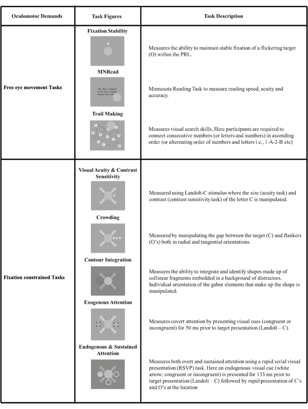
Figure 4: A visual representation of different assessment tasks designed using the framework. The tasks are broadly categorized into Free eye movement tasks, where the scotoma follows the eye movements of the participants to view targets freely (top panel), and Fixation-constrained tasks, where the scotoma needs to be placed within a central white box throughout the task (bottom panel). This figure has been modified from38. Please click here to view a larger version of this figure.
- Free eye movement tasks
NOTE: Free eye movement tasks measure participants' eye movement behavior while they perform tasks. These promote understanding of the eye's movements in the context of naturalistic tasks such as reading and visual search.- Instructional video/verbal instructions
- Present an instructional video and scripted verbal instructions to the participant prior to the calibration.
- Calibration
- Run validations of previous calibrations between tasks and additional calibrations when validations are poor, or when participants take breaks between tasks.
- Free-viewing task specific methods
- Perform free-viewing tasks that instruct participants to do a variety of actions using their gaze rather than fixating on one area. Choose to perform the task with one of the following variants.
- Bring the scotoma near a cue, causing a stimulus to appear. Maintain fixation on a specific screen location for a period of time. Perform a standard task, like reading or visual search, with central vision occluded by the scotoma.
- At the beginning of tasks, provide participants with on-screen instructions followed by a set of practice trials. Following the completion of the practice trials, give reminder instructions before moving on to the task. Ensure that the participants understand and have shown proficiency using the visual layouts, the required oculomotor actions, and the response characteristics of each task prior to measuring performance.
- Provide participants with auditory feedback indicating the accuracy of their responses as they complete each task, as visual feedback can be missed due to the use of a scotoma.
- Incorporate breaks of up to 1 min into each task to reduce the chance of testing fatigue. Incorporate breaks of 3 min or longer for days that include longer sessions of assessments to reduce the chances of testing fatigue.
- Instructional video/verbal instructions
- Fixation-constrained tasks
NOTE: Fixation-constrained tasks are useful to test or train peripheral vision at specific visual field locations. These tasks are suitable for testing both early- and mid-level visual processing, including visual acuity, contrast sensitivity, crowding, etc., as well as high-level visual processing, including exogenous and endogenous attention. For these tasks, it is important that participants learn to maintain steady fixation to avoid task performance being confounded by attentional resources dedicated to steady fixation. During these tasks, participants are asked to keep their central vision focused on the center of the screen with the help of fixation aids (Figure 5B) while responding to stimuli that appear in their peripheral vision.- Instructional video/verbal instructions
- Present an instructional video and scripted verbal instructions to the participant prior to the calibration.
- Calibration
- Run validations of previous calibrations between tasks and additional calibrations when validations are poor, or when participants take breaks between tasks.
- Fixation-constrained task-specific methods
- During fixation-constrained tasks, ask participants to maintain their head position in the chinrest for the duration of the task, ensuring that the calibration remains as accurate as possible to the original position throughout the process.
- Provide participants with on-screen instructions followed by a set of practice trials. Following the completion of the practice trials, give a reminder set of on-screen instructions before moving on to the task.
- During these tasks, ask participants to keep their central vision focused on the center of the screen with the help of fixation aids (white rectangular fixation box) while responding to stimuli that appear in their peripheral vision to either side of the fixation box.
- Ask participants to respond using their right index finger on a five-button response box located to their right during the assessment. If fixation is not maintained, the stimulus will not be presented and will time out unless fixation is resumed.
- Provide participants with auditory feedback indicating the accuracy of their responses as they complete each task, as, again, visual feedback can be missed due to the use of a scotoma.
- Incorporate breaks of up to 1 min into each task to reduce the chance of testing fatigue. Incorporate breaks of 3 min or longer for days that include longer sessions of assessments to reduce the chances of testing fatigue.
- Instructional video/verbal instructions
- Development of appropriate fixation displays
NOTE: Tasks involving peripherally presented targets and simulated scotoma obstructing central vision present challenges when trying to estimate performance in a retinotopically defined location. Indeed, even in foveal tasks, the eyes make small, involuntary movements in the form of drift and microsaccades). Thus, in order to optimize fixation stability, careful thought should go into designing fixation aids.- Develop a fixation aid design that incorporates both a large fixation cross and a fixation box (Figure 5). Instruct participants to maintain the opaque occluder within the fixation box and use the long arms of the fixation cross as a reference for the center of the screen.
NOTE: This design combines both bullseye- and crosshair- types of visual aids, which have been shown to lead to the best fixation stability39. Additionally, by having both a fixation box and a fixation cross, this design can be easily used in translational contexts to test patients with central vision loss, as is the case of patients with MD.
- Develop a fixation aid design that incorporates both a large fixation cross and a fixation box (Figure 5). Instruct participants to maintain the opaque occluder within the fixation box and use the long arms of the fixation cross as a reference for the center of the screen.
- Optimization of adaptive procedures to accurately measure performance
NOTE: A critical aspect of implementing different assessments is the ability to quickly and successfully estimate performance thresholds in a subset of these tasks (specifically visual acuity, contrast sensitivity, crowding, and contour integration). A challenge is that conventional staircases can be slow to converge and target performance close to the threshold, causing frustration and fatigue. To circumvent this, we implemented a three-stage procedure to estimate the performance of participants in these tasks.- In the first stage, ask participants to perform 12 practice trials before the actual experiment. During the second stage, utilize a 2-down 1-up staircase that terminates after 3 downward reversals (i.e., the direction of stimulus change, from down (hard) to up (easy), also refer to representative results section), followed by the third stage that consist of a conventional 3-down 1-up staircase that ends after 60 trials.
NOTE: Pilot studies indicated that this procedure achieves reliable thresholds for most tasks (visual acuity, crowding, and contrast sensitivity tasks). However, some tasks can require other methods, especially when performance can differ greatly across participants. For example, in the contour integration task, after the first stage of the procedure (practice), an additional procedure was implemented. The difficulty of the task was manipulated using a progressive staircase method where the orientation jitter (0°, 1°, 2°, 4°, 6°, 8°, 10°, 12°) increased every three trials for a total of 24 trials. Then, the second and third stages of the procedure (adaptive staircase) continued as normal. In general, different tasks may require slightly different adaptive procedures. However, the 3-stage approach allows participants to practice and quickly get within range of their threshold and provides detailed measurement within that range.
- In the first stage, ask participants to perform 12 practice trials before the actual experiment. During the second stage, utilize a 2-down 1-up staircase that terminates after 3 downward reversals (i.e., the direction of stimulus change, from down (hard) to up (easy), also refer to representative results section), followed by the third stage that consist of a conventional 3-down 1-up staircase that ends after 60 trials.
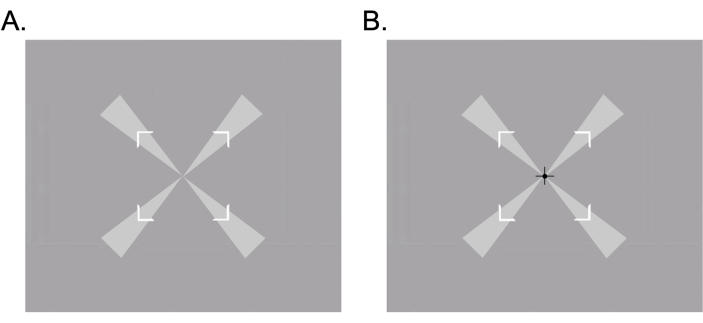
Figure 5: Fixation aids used to promote fixation stability in participants. (A) Fixation cross and fixation box were used for fixation stability tasks. (B) The fixation cross, fixation box, and black cross at the center were used in low-level vision tasks. Please click here to view a larger version of this figure.
Access restricted. Please log in or start a trial to view this content.
Results
In this section, we present illustrative data from both free eye movement and fixation-constrained tasks. The goal of this section is to illustrate data obtained using the framework and its ability to measure peripheral visual functions. The section is organized into four distinct categories, each highlighting critical elements necessary for accurate visual performance estimation under simulated central vision loss. These categories include performance on (1) low- and mid-level vision tasks, (2) attention measures in hig...
Access restricted. Please log in or start a trial to view this content.
Discussion
In this methodological paper, we present a gaze-contingent framework for conducting perceptual research in simulated central vision loss that emphasizes hardware, design, and methodological considerations that are required to (1) choose the shortest system latency for gaze-contingent display, (2) administer a wide range of visual perception tasks, and (3) measure the oculomotor and perceptual performance of participants within this paradigm. Concerning (1), we emphasize the need for testing hardware and software reliabil...
Access restricted. Please log in or start a trial to view this content.
Disclosures
The authors declare that there is no conflict of interest regarding the publication of this paper.
Acknowledgements
This work is supported by NIH NEI 1 U01 R01EY031589 and 1R21EY033623-01.
Access restricted. Please log in or start a trial to view this content.
Materials
| Name | Company | Catalog Number | Comments |
|---|---|---|---|
| CRT Monitor | ViewSonic PF817 Professional Series CRT, ViewSonic Corp. | https://www.viewsonic.com/us/monitors.html?srsltid= AfmBOorEmjc67A5U2v2V wywNRHWzdrxcYx7Q3Y0 9tiNrnbs6FC4TPlc9 | |
| Display++ LCD Monitor | Cambridge Research Systems | https://www.crsltd.com/tools-for-vision-science/calibrated-displays/displaypp-lcd-monitor/ | |
| Eye Tracker | EyeLink 1000 Plus Tower Mount, SR Research | https://www.sr-research.com/eyelink-1000-plus/ | |
| Eye Tracker | Vpixx Technologies Inc. | www.vpixx.com | |
| Macintosh IOS | Apple Inc. | https://www.apple.com/mac/ | |
| Windows 10 | Microsoft Inc. | https://www.microsoft.com/en-us/ |
References
- Wong, W. L., et al. Global prevalence of age-related macular degeneration and disease burden projection for 2020 and 2040: a systematic review and meta-analysis. Lancet Glob. Health. 2 (2), e106-e116 (2014).
- Bowers, A., Peli, E., Elgin, J., McGwin, G., Owsley, C. On-road driving with moderate visual field loss. Optom Vis Sci. 82 (8), 657-667 (2005).
- Bullimore, M. A., Bailey, I. L. Reading and eye movements in age-related maculopathy. Optom Vis Sci. 72 (2), 125-138 (1995).
- Bernard, J. B., Chung, S. T. L. The role of external features in face recognition with central vision loss. Optom Vis Sci. 93 (5), 510-520 (2016).
- Šiaudvytytė, L., Mitkutė, D., Balčiūnienė, J. Quality of life in patients with age-related macular degeneration. Medicina (Kaunas). 48, 109-111 (2012).
- Sabel, B. A., Wang, J., Cárdenas-Morales, L., Faiq, M., Heim, C. Mental stress as consequence and cause of vision loss: the dawn of psychosomatic ophthalmology for preventive and personalized medicine. EPMA J. 9 (2), 133-160 (2018).
- Fletcher, D. C., Schuchard, R. A. Preferred retinal loci relationship to macular scotomas in a low-vision population. Ophthalmology. 104 (4), 632-638 (1997).
- White, J. M., Bedell, H. E. The oculomotor reference in humans with bilateral macular disease. Invest Ophthalmol Vis Sci. 31 (6), 1149-1161 (1990).
- Whittaker, S. G., Cummings, R. W. Foveating saccades. Vision Res. 30 (9), 1363-1366 (1990).
- Sabbah, N., et al. Reorganization of early visual cortex functional connectivity following selective peripheral and central visual loss. Sci Rep. 7, 43223(2017).
- Verdina, T., et al. Efficacy of biofeedback rehabilitation based on visual evoked potentials analysis in patients with advanced age-related macular degeneration. Sci Rep. 10, 20886(2020).
- Verdina, T., et al. Biofeedback rehabilitation of eccentric fixation in patients with Stargardt disease. Eur J Ophthalmol. 23 (5), 723-731 (2013).
- Nilsson, U. L., Frennesson, C., Nilsson, S. E. Location and stability of a newly established eccentric retinal locus suitable for reading, achieved through training of patients with a dense central scotoma. Optom Vis Sci. 75 (12), 873-878 (1998).
- Morales, M. U., et al. Biofeedback fixation training method for improving eccentric vision in patients with loss of foveal function secondary to different maculopathies. Int Ophthalmol. 40 (2), 305-312 (2020).
- Nilsson, U. L., Frennesson, C., Nilsson, S. E. Patients with AMD and a large absolute central scotoma can be trained successfully to use eccentric viewing, as demonstrated in a scanning laser ophthalmoscope. Vision Res. 43 (16), 1777-1787 (2003).
- Tarita-Nistor, L., Brent, M. H., Steinbach, M. J., Markowitz, S. N., González, E. G. Reading training with threshold stimuli in people with central vision loss: a feasibility study. Optom Vis Sci. 91 (1), 86-96 (2014).
- Maniglia, M., et al. Perceptual learning leads to long lasting visual improvement in patients with central vision loss. Restor Neurol Neurosci. 34 (5), 697-720 (2016).
- Maniglia, M., Soler, V., Trotter, Y. Combining fixation and lateral masking training enhances perceptual learning effects in patients with macular degeneration. J Vis. 20 (10), 19(2020).
- Chung, S. T. L. Improving reading speed for people with central vision loss through perceptual learning. Invest. Ophthalmol Vis Sci. 52 (2), 1164-1170 (2011).
- Plank, T., et al. Perceptual learning in patients with macular degeneration. Front Psychol. 5, 1189(2014).
- Xie, X. Y., Liu, L., Yu, C. A new perceptual training strategy to improve vision impaired by central vision loss. Vision Res. 174, 69-76 (2020).
- Fine, E. M., Rubin, G. S. Reading with simulated scotomas: attending to the right is better than attending to the left. Vision Res. 39 (5), 1039-1048 (1999).
- Costela, F. M., Reeves, S. M., Woods, R. L. Orientation of the preferred retinal locus (PRL) is maintained following changes in simulated scotoma size. J Vis. 20 (7), 25(2020).
- Chen, N., et al. Cortical reorganization of peripheral vision induced by simulated central vision loss. J. Neurosci. 39 (18), 3529-3536 (2019).
- Bertera, J. H. The effect of simulated scotomas on visual search in normal subjects. Invest Ophthalmol Vis Sci. 29 (3), 470-475 (1988).
- Barraza-Bernal, M. J., et al. Can positions in the visual field with high attentional capabilities be good candidates for a new preferred retinal locus. Vision Res. 140, 1-12 (2017).
- Kwon, M., Nandy, A. S., Tjan, B. S. Rapid and persistent adaptability of human oculomotor control in response to simulated central vision loss. Curr Biol. 23 (17), 1663-1669 (2013).
- Liu, R., Kwon, M. Integrating oculomotor and perceptual training to induce a pseudofovea: A model system for studying central vision loss. J Vis. 16 (6), 10(2016).
- Maniglia, M., Jogin, R., Visscher, K. M., Seitz, A. R. We don't all look the same; detailed examination of peripheral looking strategies after simulated central vision loss. J Vis. 20 (13), 5(2020).
- Walsh, D. V., Liu, L. Adaptation to a simulated central scotoma during visual search training. Vision Res. 96, 75-86 (2014).
- Van der Stigchel, S., et al. Macular degeneration affects eye movement behavior during visual search. Front Psychol. 4, 579(2013).
- Maniglia, M., Visscher, K. M., Seitz, A. R. Perspective on vision science-informed interventions for central vision loss. Front Neurosci. 15, 734970(2021).
- Aguilar, C., Castet, E. Gaze-contingent simulation of retinopathy: some potential pitfalls and remedies. Vision Res. 51, 997-1012 (2011).
- Lin, Z., Yang, Z., Feng, C., Zhang, Y. PsyBuilder: An Open-Source, Cross-Platform Graphical Experiment Builder for Psychtoolbox With Built-In Performance Optimization. Adv Meth Pract Psychol Sci. 5, 251524592110705(2022).
- Bridges, D., Pitiot, A., MacAskill, M. R., Peirce, J. W. The timing mega-study: comparing a range of experiment generators, both lab-based and online. PeerJ. 8, e9414(2020).
- Rohr, M., Wagner, A. How monitor characteristics affect human perception in visual computer experiments: CRT vs. LCD monitors in millisecond precise timing research. Sci Rep. 10, 6962(2020).
- Saunders, D. R., Woods, R. L. Direct measurement of the system latency of gaze-contingent displays. Behav Res Methods. 46 (2), 439-447 (2014).
- Jayakumar, S. Developing robust methods and tools for advancing perceptual learning research. , UC Riverside. https://escholarship.org/uc/item/7gk9r0q3 (2024).
- Thaler, L., Schütz, A. C., Goodale, M. A., Gegenfurtner, K. R. What is the best fixation target? The effect of target shape on stability of fixational eye movements. Vision Res. 76, 31-42 (2013).
- Gaudino, E. A., Geisler, M. W., Squires, N. K. Construct validity in the Trail Making Test: What makes Part B harder. J Clin Exp Neuropsychol. 17 (4), 529-535 (1995).
- Crossland, M. D., Culham, L. E., Rubin, G. S. Fixation stability and reading speed in patients with newly developed macular disease. Ophthalmic Physiol Opt. 24 (4), 327-333 (2004).
- Maniglia, M., Visscher, K. M., Seitz, A. R. A method to characterize compensatory oculomotor strategies following simulated central vision loss. J Vis. 20 (9), 15(2020).
- Agaoglu, M. N., Fung, W., Chung, S. T. L. Oculomotor responses of the visual system to an artificial central scotoma may not represent genuine visuomotor adaptation. J Vis. 22 (10), 17(2022).
- Frennesson, C., Jakobsson, P., Nilsson, U. L. A computer and video display based system for training eccentric viewing in macular degeneration with an absolute central scotoma. Doc Ophthalmol. 91 (1), 9-16 (1995).
- Fletcher, D. C., Schuchard, R. A., Renninger, L. W. Patient awareness of binocular central scotoma in age-related macular degeneration. Optom Vis Sci. 89 (9), 1395-1398 (2012).
- Harrar, V., Le Trung, W., Malienko, A., Khan, A. Z. A nonvisual eye tracker calibration method for video-based tracking. J Vis. 18 (9), 13(2018).
- Ramírez Estudillo, J. A., et al. Visual rehabilitation via microperimetry in patients with geographic atrophy: a pilot study. Int J Retina Vitreous. 3, 21(2017).
Access restricted. Please log in or start a trial to view this content.
Reprints and Permissions
