Multimodal Analysis of Microplastics in Drinking Water using a Silicon Nanomembrane Analysis Pipeline

Summary

Here, we present a protocol showcasing an optically transparent and flat substrate for the streamlined capture and analysis of contaminating particles in drinking water. Presented here is the Silicon Nanomembrane Analysis Pipeline (SNAP): a flexible pipeline for the capture, quantification, and identification of particles in liquid media.

Abstract

The biological impact of microplastic pollution in human food and water sources is largely unknown, and drinking water sources are not exempt from this microplastic contamination. Here, we demonstrate a streamlined approach for capturing, quantifying, and identifying microplastics in drinking water. We present an analytical workflow termed the Silicon Nanomembrane Analysis Pipeline (SNAP) that takes advantage of novel Silicon nitride nanomembranes that enable a significant "concentration factor," which consolidates suspended particles into a planarized observation area for individuated, quantifiable, and multimodal particle analysis on the same substrate. SNAP's primary advantages derive from its use of ultrathin, Silicon nitride-based membranes housed in conventionally sized filter disks, enabling the direct capture and analysis of polymeric MPs on a non-polymeric background. Drinking water samples sourced in the Rochester, NY region, were collected from residential tap sources and analyzed using SNAP. Particles in each sample were characterized by optical and scanning electron microscopy (SEM), Raman spectroscopy, and energy-dispersive X-ray spectroscopy (EDX), and various identified constituents were quantified in proportion to the total captured particles.

Introduction

Microplastics are defined as synthetic polymers measuring smaller than five millimeters in size^1,2. Microplastic (MP) pollution is a growing human health, environmental, and ecological concern. MP contamination has been found in water sources of all types; freshwater, oceans, and even drinking water sources³. MPs are generated from the breakdown of primary plastic sources⁴, as well as synthetic textiles^5,6,7. MPs are ubiquitous and have been found in human tissues, such as human placenta, feces, and blood^8,9,10. There is an increasing interest in MP research, as evidenced by more than 4,100 and 4,600 publications in 2023 and 2024, respectively (PubMed data; keyword "microplastics"), as well as an increasing public concern regarding human exposure to MPs. Responding to a growing public concern, several government regulatory bodies such as the State of California¹¹ and several EU countries¹², have been (or will be) implementing regulations on MP levels in drinking water. Considering all of the above, the US Environmental Protection Agency has recently announced MPs as a new contaminant of concern. However, human risk evaluation is severely impeded by a lack of methods for the reliable and reproducible detection of MPs.

Characterization of MPs relies on analytical methods such as optical and electron microscopy¹³, and spectroscopic and spectrometric techniques^1,14,15 to understand the visual characteristics of MPs⁷ and their composition, respectively. Samples containing MPs should include multiple analyses to characterize, identify, and quantify MPs, and at least require spectroscopy/spectrometry (i.e., Raman spectroscopy, infrared spectroscopy, or pyrolysis gas chromatography-mass spectrometry, etc.) as per some journal minimal requirements for the measurement of plastics in environmental samples, such as Science of the Total Environment¹⁶. Raman spectroscopy is more versatile than infrared (IR) spectroscopy, especially with respect to material identification in biological samples. Raman spectroscopy is a light scattering technique, enabling it to analyze smaller particles more easily than IR, a light-absorbing technique that necessitates larger particles and has more constraints on sample placement¹⁷. It has been previously suggested that substrates for Raman spectroscopy comprising Silicon or Silicon oxide can yield reliable results with minimal background noise¹⁸.

Substrates for certain analytical techniques that are usually compatible with one type of analysis (i.e., Gold-coated substrates required for IR spectroscopy) are not often compatible with transmission and/or reflectance light microscopy. Subsequently, replicate subsampling is popular among investigators to produce samples appropriate for each separate analysis, but subsampling is time-consuming and could exclude low-abundance particulates^1,2,6. Typically, manual transfers of particulates from one substrate to the next is necessary to analyze the same particle for characterization and identification by different analytical modalities, but these slow, manual transfers increase the likelihood of bias, contamination, and loss, as well as limit analysis of MPs to only the largest sized particles that can be manually manipulated¹³. These suboptimal workflows introduce numerous challenges and reliability issues, contributing to the significant variability in MP quantification reported in the literature^3,7.

Here, we present an analytical workflow we call the Silicon Nanomembrane Analysis Pipeline (SNAP) to capture, characterize, identify, and quantify MPs, and demonstrate the utility of SNAP by analyzing drinking water samples sourced from the Rochester, NY region. SNAP is enabled by conventionally sized 25 mm diameter filter disks with integrated Silicon nanomembranes (See Supplemental Table S1 for membrane properties), which offer a uniform substrate for concentrating and analyzing MPs from drinking water using multiple techniques^15,19. After sequentially concentrating and capturing MPs onto nanomembranes with decreasing cut-off sizes (20 µm microporous Silicon nitride (MPSN) with cylindrical pores and 8.0 µm microslit Silicon nitride (MSSN) with rectangular prism pores), SNAP facilitates three consecutive analytical steps: 1) sample staining, optical microscopy, and MP quantification, 2) particle identification via Raman spectroscopy, followed by 3) particle characterization via scanning electron microscopy (SEM), enabling multiple analyses of the same particles captured onto one nanomembrane substrate.

We demonstrate multiple SNAP pipelines by utilizing both uncoated Silicon nanomembrane (SiN) filter disks and Gold coated Silicon nanomembrane (Au-SiN) filter disks: Pipeline A) SNAP performed on SiN and sequentially characterizing the same MPs through multiple analytical techniques; Pipeline B) SNAP performed on Au-SiN with Raman spectroscopy; and Pipeline C) SNAP performed on Au-SiN with SEM equipped with energy dispersive X-ray spectroscopy (EDX) (Figure 1). SNAP variations are thus flexible, streamlined analytical workflows that can be used for a number of sample types and analytical techniques. Unlike previously published methods that rely on polymeric membranes¹¹, SNAP's advantages derive from its use of Silicon nanomembranes, where synthetic polymer MPs are captured onto a non-polymeric, Silicon-based membrane, enabling the compositional identification of MPs on a non-polymeric background. Further, Silicon nanomembranes offer uniform focal planes unlike polymeric membranes, which tend to wrinkle, enabling multiple automated microscopy and spectroscopy techniques.

We previously characterized the use of Silicon nanomembranes for MP analyses by analytical modeling, model particle challenges, and drinking water and air samples^19,20, as well as by comparing their filtration and optical microscopy properties using model particles against four widely used membranes¹⁵. In this protocol, we heuristically demonstrate SNAP's utility for the analysis of MPs in four drinking water samples. Samples were collected from four distinct water sources around the greater Rochester, NY area. Each sample included in this study originated from a distinct surface water source, such as Lake Ontario, Hemlock Lake, a mix of Hemlock and Ontario, and Canandaigua Lake (Figure 2). Captured particles from these drinking water sources included widespread plastics like polystyrene (PS) and polyethylene (PE), heavy metals like iron, silica, and non-synthetic particles.

Protocol

1. Quality control procedures and Ultrapure solution preparations

1. Laminar flow hood and glove cleaning
   1. Don PPE (personal protective equipment): 100% cotton lab coat and nitrile gloves.
      NOTE: PPE is continuous throughout the protocol.
   2. Spray Nitrile gloves with 99% Isopropyl alcohol (IPA). Rub hands together, and then rinse with ~18 MΩ, 0.22 µm-filtered water. Do this 3x to remove the release agent from the gloves.
   3. Fold a natural fiber delicate task wipe into quarters, then spray with 70% IPA. Wipe the hood surface from back to front in long strokes, re-folding the delicate task wipe to an unused surface every two strokes. Continue cleaning the hood until all surfaces have been cleaned, replacing the wipe with a new one once it has been soiled.
   4. Uncover the silicone roller mat, and roll across the surface of the hood to pick up any remaining particles. To clean the silicone roller, spray with 99% IPA and scrub with a gloved hand, then rinse with 18 MΩ, 0.22 µm-filtered water. Repeat 3x, then allow to air-dry in the hood.
   5. Re-rinse gloves as in step 1.1.2.
2. Ultrapure water and IPA generation.
   1. Fill a 1 L beaker with 18 MΩ water and place it in the hood.
   2. Prime a 60 mL syringe and attached 0.22 µm cut-off syringe filter by filtering at least 200 mL of 18 MΩ water through the syringe and attached filter.
      NOTE: A syringe pump will save time but is not a requirement to carry out the described protocol.
   3. Rinse a glass screw-cap container 3x with 18 MΩ, 0.22 µm-filtered water. Fill with 0.22 µm syringe-filtered 18 MΩ filtered water.
   4. Repeat steps 1.2.1-1.2.3 with the desired % concentration of IPA instead of 18 MΩ, 0.22 µm-filtered water to generate ultrapure IPA.

2. Particle capture from liquid samples via filtration

NOTE: The protocol below may be utilized with liquid samples other than water. Validated sample collection methods should be left up to the discretion of the investigator based on the needs of their study and of the sample.

1. Don PPE.
   NOTE: Ensure gloves and hood surfaces are cleaned in accordance with steps 1.1.2-1.1.5.
2. Spray a silicone gasket with Ultrapure 99% IPA, scrub with gloved fingers, then rinse with Ultrapure water. Repeat this 3x for each gasket.
   NOTE: The number of gaskets to be used in filtration equals the number of filter disks to be used, plus 1. Refer to Figure 1B for the visual assembly graphic.
3. Utilizing the syringe primed in step 1.1.2, rinse the inside of the 60 mL syringe with the Ultrapure water by taking up 30 mL of Ultrapure water and 30 mL of air into the syringe. Screw on a syringe filter, then shake vigorously and dispense. Repeat this 3x.
   NOTE: Any sized syringe may be utilized as necessary based on the sample's volume.
4. Assemble the filtration apparatus as shown in the visual assembly graphic in Figure 1B.
   NOTE: Use clean tweezers to handle filter disks and gaskets during assembly and disassembly.
   1. For sequential filtrations, ensure that there is a gasket between the disk and the support frit, a gasket between each disk, and a gasket between the disk and the filtration funnel.
   2. Ensure that the disks are ordered with the largest cut-off filter at the top of the stack and the smallest cut-off filter on the bottom.
5. Turn on the vacuum to the apparatus so that there is negative flow through the filter disk stack.
6. Measuring background contamination
   NOTE: The following process enables an evaluation of the syringe cleaning and the Ultrapure media generation, and a determination of background particles contributed by the system's components.
   1. With the rinsed syringe, dispense 50 mL of Ultrapure water slowly over the nanomembrane in the center of the top disk to ensure that all the dispensed liquid is filtered.
      NOTE: If filtering larger sample volumes (i.e., >50 mL), a glass filtration funnel is suggested. Clean the glass filtration funnel as in step 2.3. Additional labware may incur additional particle contamination risk. Maintain diligence with cleaning procedures and always confirm cleanliness with blank filtrations prior to using the samples of interest.
   2. Allow the ultrapure water to filter. Keep the vacuum on for one additional minute post filtration. Once the sample is fully dry, turn off the vacuum.
   3. Carefully remove the filter disks from the gaskets using clean tweezers and place disks into the appropriate clean and labeled container for storage, such as a glass Petri dish or darkened box.
   4. Image the filter disks under microscopy for optical analysis, particle counting, etc.
7. For liquid samples, clean an additional gasket as in step 2.2. Obtain a new syringe for each unique liquid media sample and repeat step 2.3.
8. Uptake the desired amount of sample and dispense the sample slowly over the nanomembrane in the center of the top disk.
9. Once sample filtration is complete, conduct 3x rinses with 1 mL of Ultrapure water to ensure all particles in the sample have been sufficiently rinsed from all surfaces onto the membrane at the center of the filter disk.
10. Keep the vacuum on for one additional minute to fully dry the 3x-rinsed sample, then turn off the vacuum.
    1. Repeat steps 2.7-2.10. for each replicate to be performed of the sample of interest.

3. Fluorescent dye preparation and staining

NOTE: Fluorescent staining with Nile Red and/or Trypan Blue may interfere with Raman spectroscopy lasers of interest.

1. Staining with Nile Red (NR)
   1. Don PPE.
   2. Clean gloves and hood as in steps 1.1.2-1.1.5.
   3. Complete sample filtration as outlined in steps 2.7-2.10.
   4. Rinse two glass screw cap containers with Ultrapure water 3x.
   5. Prepare a 0.1 mg/mL solution of NR in Ultrapure 99% IPA in a clean glass container.
   6. Gently invert 10x to mix.
   7. Filter the NR solution with a 0.22 µm syringe filter into the second glass screw cap container.
      NOTE: The filter used to prefilter the NR should have a smaller cutoff than the filter used to filter the samples.
   8. Place the filter disk to be stained onto the support frit of the vacuum collection flask.
   9. Pipette 20 µL of the 0.1 mg/mL NR solution onto the nanomembrane at the center of the filter disk.
      NOTE: The stain should fully cover the porous surface of the nanomembrane. If 20 µL is not enough, add additional stain until all porous areas of the nanomembrane are suitably covered in stain.
   10. Incubate the stain for 5 min.
   11. Vacuum filter the stain once the incubation is complete.
   12. Rinse 3x with 1 mL of Ultrapure 99% IPA to remove any excess NR stain.
       NOTE: Proceed to the Trypan Blue staining section below after this step if counterstaining is to be performed.
   13. Allow the filter disk to sit on the support frit with the vacuum on for 2 min to filter and dry any residual liquid. If not dry after 2 min, transfer the filter disk using a clean glass Petri dish to a 70 °C oven for 2-5 min.
   14. Once dry, perform fluorescence microscopy as described in step 2.6.4  and proceed to section 4.
2. Staining with Trypan Blue (TB)
   1. Don PPE.
   2. Clean gloves and hood as outlined in steps 1.1.2-1.1.5.
   3. Complete sample filtration from steps 2.7-2.10 or begin with step 3.2.4.
   4. Rinse two glass screw cap containers with Ultrapure water 3x.
   5. Prepare 0.4% TB stain in one container.
      NOTE: The filter used to prefilter the TB should have a smaller cutoff than the filter used to filter the samples.
   6. Gently invert 10x to mix.
   7. Filter the TB stain solution with a 0.22 µm syringe filter into the second glass screw cap container.
      NOTE: The filter used to prefilter the TB should have a smaller cutoff than the filter used to filter the samples.
   8. Place the filter disk to be stained onto the support frit of the vacuum collection flask.
   9. Pipette 20 µL of the 0.4% TB stain onto the nanomembrane at the center of the filter disk.
      NOTE: The stain should fully cover the porous surface of the nanomembrane. If 20 µL is not enough, add additional stain dropwise until all porous areas of the nanomembrane are suitably covered in the stain.
   10. Incubate the stain for 5 min.
   11. Vacuum filter the stain after incubating for 5 min.
   12. Rinse with 1 mL volumes of Ultrapure water 3x.
   13. Allow the filter disk to sit on the support frit with the vacuum on for 2 min to filter and dry any residual liquid. If not dry after 2 min, transfer the filter disk using a clean glass Petri dish to a 70 °C oven for 2-5 min.
   14. Once dry, perform fluorescence microscopy as described in step 2.6.4 and proceed to section 4.

4. Particle quantification via fluorescence microscopy

1. Optical microscopy image capture
   1. Immobilize the filter disk on a microscope slide using a silicone gasket, or utilize an alignment slide specific to filter disk use with a microscope stage. Move the filter disk to be imaged to the microscope stage.
   2. Image the nanomembrane using brightfield illumination so that the maximum detected counts are ~ 90% of the detector camera's maximum range.
      NOTE: This 90% value is ~59,000 for a 16-bit detector with white levels at 65,535.
   3. Image the nanomembrane using fluorescent illumination so the maximum pixel intensities are around ~25% of the detector camera's maximum range.
   4. Save the image in a 16-bit composite TIFF format.
2. Particle quantification via fluorescence microscopy
   1. Using the image analysis platform, separate the fluorescent channel(s) of the composite TIFF generated in 4.1.4 from the brightfield channel using the Split-Channels function.
   2. Threshold the pixel intensities using the Threshold function to a value of 10,000.
      NOTE: If bloom is present on the particles, the threshold is too low and should be raised.
   3. Save a separate image in PNG format.
   4. Despeckle the image to remove noise pixels using the Despeckle function.
   5. Watershed the image using the Watershed function.
      NOTE: This function separates adjoining particles of a similar size, at the cost of breaking up large contiguous particles into smaller pieces. As there are often many more small particles than large particles present, this can be a good tradeoff but can have unintended effects, such as breaking up long fibers into strands of small particles. Inspect image results before accepting data.
   6. Set the scale of the thresholded fluorescent images by measuring the width of a pore in the brightfield image. Use the measured pore width to Set the Scale in pixels/µm.
      NOTE: For rectangular pores, the smallest width will match the product label. For circular pores, the diameter will match the product label specifying the pore size (i.e., cut-off) of the nanomembrane.
   7. Apply the image analysis platform's Count Particles function to the thresholded fluorescent image, evaluating the Area, min, and max.
   8. Process the fluorescent and brightfield images to create composites that visualize the fluorescent domains.
   9. Threshold the fluorescent image using the same value as in step 4.2.2.
   10. Merge channels using the image analysis platform. Assign the fluorescent channel to the Red channel and the brightfield image to the Grays channel.
   11. Save the composite as a PNG file.

5. Raman Spectroscopy

1. Turn on the Raman instrument and its associated computer, allowing each to start up.
2. Open the software on the computer connected to the Raman instrument.
3. When the software is initialized, ensure that the Current System Activity and Detector status on the bottom ribbon of the program screen read Ready and are the color green, respectively.
4. If the Autocalibration (AC) button at the bottom of the screen is red, run the desired autocalibration and allow it to finish before continuing.
5. If only utilizing one laser and one grating:
   1. Click Exit on the Autocalibration screen, then select the desired laser and grating from their respective dropdown lists under Instrument Setup in the Acquisition tab.
   2. Return to the red AC button on the bottom of the screen and click Current laser/Grating and allow the calibration routine to run.
6. If utilizing all lasers and gratings, simply select All Lasers and Gratings and allow the system to run.
7. If utilizing more than one laser and/or grating, select the Custom lasers/Gratings and select all the desired settings. Then, allow the calibration to run.
8. Select the 20x long working distance (LWD) objective on the instrument turret, and within the software under Instrument Settings in the Acquisition tab.
9. If this objective is not available, use an alternative low magnification objective (e.g., 5x or 10x) with a working distance that accommodates the height of the filter disk.
   NOTE: Begin with a lower magnification objective to make initial navigation across the filter disk's nanomembrane easier.
10. Place the filter disk onto the microscope stage so that it is within the optical path.
11. Click Video Acquisition in the top ribbon to turn on the visualization optics.
12. Utilize the coarse and fine focus wheels on the instrument to bring the filter disk's nanomembrane into focus.
13. Roughly square the pores with the point cursor lines on the computer screen.
14. Either gently rotate the filter disk on the stage to achieve this squared alignment, or utilize an alignment slide specific for filter disk use in a microscope stage.
15. Under the Acquisition tab at the top right, ensure that the illuminator mode selected is Dark field for best results.
16. To acquire a stitched image, navigate to the Video tab in the Data Tabs ribbon.
17. Navigate to the first desired field of view, then click the Mosaic button at the top right of the video window and add to the map. Navigate to the outer opposite corner of the desired area with the instrument joystick and add to the map.
18. Run the mosaic acquisition with ViewSharp to ensure that all areas are properly in-focus in the final image.
    NOTE: Lower magnification objectives will take less time for the image mosaic acquisition, while higher magnification objectives will take longer.
19. Once the image mosaic has been created, right-click the image and hit Send to ParticleFinder.
20. Navigate to the ParticleFinder tab in the top right ribbon to interact with the thresholding settings.
21. To ensure that the proper particles are selected, left-click Image under the ParticleFinder data tab to check the Center, Particle and Transparency boxes. Set the transparency slider to 50%, and the pixel size of Center to 2px.
    NOTE: The Center selection will place a dot on the center of each particle, and the Particle selection will place an overlay over each area determined to be a particle, at 50% transparency. These settings will locate each particle and define each particle's edges.
22. If needed, edit the particle thresholding and morphology/size selection parameters under the ParticleFinder tab on the right side of the program to ensure all particles and their size/shape parameters are properly identified. Refer to Supplemental Table S2 for an example of how the morphological parameters can be applied.
    1. If automatic particle detection is not sufficient, switch to manual and incrementally adjust the thresholding values until a majority of the correct objects are identified as particles.
    2. If the morphology of the detected particles needs further refinement, check the box next to Apply morphological filters. Select suitable parameters and their intensities in the resultant dropdown menus.
       NOTE: The order in which the parameters are selected in can impact the output.
23. If the size, shape, or other morphological qualities of the particles are critical factors, check the box next to Apply particles pre-filter, then select and edit parameters as needed.
24. Once the particles have been identified and their selected shapes/edges are acceptable, navigate the scrollable preview list of particle images under the Results section. Select particle(s) of interest by clicking the associated particle image.
25. Turn on the live view with the video camera button on the top of the screen.
26. Switch to the 50x LWD objective by clicking the magnification number and selecting the corresponding objective in the dropdown menu, within the application at the bottom ribbon.
27. Bring the particle(s) back into focus with the fine adjustment knob, if necessary.
28. Capture images of individual particles o be analyzed with Raman spectroscopy, and save the images as separate files with appropriate names.
29. Ensure that the desired area of the particle to be analyzed with Raman spectroscopy is positioned correctly under the laser beam location.
30. Once the proper area of the particle is selected for analysis, hit the STOP ALL button at the top of the window to turn off the visualization optics.
31. Set the laser to 532 nm, at 1% power for unstained particles, and at 785 nm or 830 nm for fluorescently stained particles.
32. Set acquisition time to 10 s and the accumulations to 5.
33. Select the Spectra tab from the data tabs menu, then press the play button to launch the Real Time Display (RTD).
    NOTE: Utilize the information obtained during RTD to optimize the settings.
34. Once satisfied with the settings and the results, hit STOP ALL to stop the RTD.
35. The final acquisition can now be collected by pressing the circle Spectrum Aquisition button beside the RTD button.
36. Save the collected spectra as separate files with appropriate names.
37. Repeat steps 5.28-5.36. for each particle of interest.
38. When finished with the sample, remove the filter disk and return the objective to the 20X LWD both manually on the scope and within the software.
39. Repeat step 5.10-5.37 for new sample(s).

6. Spectral identification

1. If a purchased or self-built Raman spectral database is not available, navigate to the open-source spectroscopy library at: https://www.openanalysis.org/openspecy/
   NOTE: OpenSpecy is an open-source Raman and IR spectroscopy database that includes 636 spectra from three different libraries of 276 polymers and materials applicable to identifying environmental MPs and fibers²¹. Pre- and post-processed spectral data are equally viable for use with this resource.
2. Save Raman spectra as individual .csv files.
   1. Label Column A as wavenumber followed by the wavenumbers of the spectra, and column B should be labeled Intensity followed by the peak intensity values per wavenumber.
3. Open the spectra by dragging and dropping the .csv file to the Browse bar at the top left.
4. Turn on Preprocessing and Identification.
5. Under Preprocessing, turn on Threshold Signal Noise, Min-Max Normalize, Smoothing/Derivative, Conform Wavenumbers, and Baseline Correction.
   NOTE: The specific settings therein can be adjusted depending on the individual characteristics of the spectra being analyzed.
6. Under Identification, select Raman as the spectrum type, and Derivative as the Library Transformation.
   NOTE: This library can be used for IR spectroscopy as well. The analysis window will show a white spectrum, the uploaded spectrum for analysis, and a red spectrum, the suspected identification match.
7. With any spectra that does not return a match r > 0.70, or reasonable peak shape correlations, utilize the top 5 suggested results as a place to begin researching potential matches as preferred.
8. Ensure that the measured peak values are within ±10 wavenumbers of a corresponding peak in the selected reference spectra before confirming a match for that peak.
9. Record spectral correlations, their correlation values, and the database from which the suspected match originates.
10. Download files according to individual needs.

7. Scanning electron microscopy

NOTE: If not metal coating the filter disk before SEM analysis, skip to section 7.2.

1. Metal coating of samples for SEM
   1. Mount the filter disk on a steel SEM stub using carbon tape.
   2. Insert into a sputterer and pump down the chamber to 50 mTorr.
   3. Open the sputtering Ar (Argon) isolation valve.
   4. Purge the system by introducing Ar into the chamber via needle valve to a 300 mTorr pressure, then evacuate the chamber down to 50 mTorr. Repeat 3x.
   5. Adjust final pressure to 100 mTorr via needle valve.
   6. Using an Au target, deposit Au on the filter disk via sputtering.
      NOTE: Other target sources (e.g., Pt, Ir, Si, etc.) may alternatively be used instead of Au; 20 mA current produces 0.1 Angstroms/s of deposition at 100 mTorr.
   7. Vent the system and remove the filter disk. Keep the filter disk adhered to the stainless steel stub.
2. SEM image capture
   1. Fasten the stub to multi-stage Zeiss Auriga holder with a set screw.
   2. Turn on the SEM and the computers that run it, and allow each to start up.
   3. Open the software attached to the SEM.
   4. Verify that the system is under vacuum (5e-6 Torr).
   5. Vent the loadlock by pressing Vent on the main body of the loadlock chamber, and open the loadlock.
   6. Mount the multi-stage holder to the teflon coated insertion jig and fasten the transfer arm using the attached screw plate.
   7. Close the loadlock, and pump down the loadlock by pressing Store on the loadlock chamber main body.
      NOTE: Completion occurs when the green lights stop flashing on the Store button.
   8. Load the multistage holder onto the stage in the main observation chamber by opening the transfer gate.
   9. Press Transfer on the main body of the load lock. The gate will drop and expose the inner chamber.
   10. Insert the loadlock arm (screwed into the multistage holder) and fix the multistage holder to the stage.
   11. Unscrew the loadlock transfer arm and retract the arm fully so that it resides in the loadlock.
   12. Close the transfer gate by pressing Transfer.
   13. Open the isolation valve by pressing EHT on in the bottom right corner of the software.
   14. Adjust the working distance to be 5 mm in the data zone of the software, and the accelerating voltage to be 20 kV.
   15. Localize the filter disk membrane using the XY and Z joysticks.
   16. Raise the stage using the Z joystick until the image comes into focus.
   17. Correct for astigmatism by adjusting the XY stigmator knobs and focus wheel on the central console.
   18. Image sample particles at desired magnification by adjusting the magnification wheel on the central console, capturing 2,048 x 1,536 resolution images in 8 or 16-bit tiff format.
3. EDX particle analysis
   1. Turn off the ChamberScope CCD on the desktop of the SEM computer.
      NOTE: If this step is not complete, the EDX detector will be overwhelmed with signal and no data will be recorded.
   2. Cool the EDX detector by opening the APEX EDX software on the EDX computer, by powering on the detector in the top right corner menu.
   3. Capture a low-resolution SEM image that can be used for mapping, by clicking Capture Image.
   4. Open the Mapping Tab menu at the top of the software screen.
   5. Under Settings, adjust the resolution (256 x 256) and pixel dwell time (0.16 µs), and frame number (32-64) to provide an estimated time of capture that should be ~5 min long.
   6. Click Create Map in the top left corner of the menu.
   7. Select Confirm Element Preview to manually adjust the element search, or rely on the Auto Identified peaks from the software.
   8. Generate a report using the AutoReport function in the top right section of the mapping software upon completion.

Results

Process blanks and background contamination
An acceptable blank result is one that contains either no particles or so few particles that the background (i.e., process) contamination (if any) does not run a high likelihood of confusing or disrupting the results of the experiment. A suboptimal blank result is one that contains many particles that the particles of interest will be difficult to distinguish from the background contamination.

The acceptable level of process contamination should be at or as close to zero as possible, but if zero cannot be achieved, then consistency in the number of observed background particles is key. Run several blank samples to determine the consistency of results. Diligence in quality control protocols (refer to Section 1), contamination mitigation, and proper environmental conditions during processing are paramount to maintaining low background contamination levels. Background contamination results and acceptability may also depend heavily upon the cut-off of the nanomembranes being used, and the overall cleanliness of laboratory conditions. Take into account that when analyzing for smaller particles with lower cut-off membranes (e.g., < 8 µm), the relative abundance of the particles of interest and similarly sized background contaminants will both increase exponentially, necessitating higher levels of stringency in quality control be applied²². While any level of contamination is not acceptable, as long as conditions are tightly controlled and a high degree of consistency is achieved, good analyses of environmental microplastics or analytics of interest may still be performed.

Sample filtration
An ideal sample filtration is needed to generate a faithful multimodal analysis, as shown with the example data cascade in Figure 3. Such sample filtration will result in well-dispersed particles across the nanomembrane surface (e.g., with approximately one-third of membrane surface area coverage). Poorly dispersed particles, such as the case with particle aggregation (large clumps of overlapping particles), will confuse both manual and automated particle counting methods, as overlapping particles are not easily differentiated with confidence. Such data is usually excluded from analysis, which may lead to the loss of valuable information of interest. Well-dispersed particles, as shown in Figure 4A,B, ensure that any spectroscopic or quantification analyses are not complicated by stacked or overlapping particles of varying compositions, which could return results that are more difficult to accurately interpret, identify, and quantify.

Nile Red and Trypan Blue staining
Representative images of optimal fluorescent particle staining instances are shown in Figure 3B on a 20 µm cut-off SiN filter disk. Under-rinsing of the NR or TB stain from the nanomembrane surface may create false positive results. Residual particulates that are comprised of either stain retained on the membrane's surface due to insufficient rinsing may be falsely interpreted as stained particles. A sign that insufficient rinsing occurred is if areas of the nanomembrane without particles or detectable residual films/residues from the filtered sample are fluorescing during observation, as shown in Figure 5A. After imaging, as long as the filter disk was maintained in clean conditions, a re-rinse may be conducted by placing the individual nanomembrane filter disk back onto the vacuum filtration apparatus (minus the gaskets), turning on the vacuum, and filtering another volume of Ultrapure 99% IPA (for NR) or Ultrapure water (for TB) onto the filter disk's nanomembrane. Record the total volume of additional rinsing media used. For best results, take microscopy images of the entire nanomembrane surface before conducting a re-rinse to account for any contamination potentially incurred by the re-rinse step.

Raman spectroscopy
Raman spectroscopy performed on non-coated SiN may produce a prominent peak depending on the laser wavelength, and this peak may mask low abundance signals approximately within the 520 cm^-1 wavenumber region²³. If Raman spectra of interest are sufficiently separated from the Silicon or Silicon Nitride background peak, using non-coated SiN filter disks should yield adequate Raman spectroscopy results. In this report, Pipelines B and C both used Au-SiN filter disks. The Gold coating of Au-SiN masks the inherent Si peak, allowing low abundance spectra to be collected more reliably near or at 520 cm^-1 wavenumbers. Additionally, Au-SiN can be used with IR spectroscopy if Raman is not available. Always start with the lowest power settings (i.e., laser intensity) on the instrument and then gradually increase, as some particles of interest can be fragile, such as oxidized particles, and may be damaged or destroyed by the laser.

When analyzing chosen particles with Raman spectroscopy, determining the reliability of a returned spectrum is crucial. Some particles may auto-fluoresce, and this fluorescence will add noise into the spectral measurement that may mask or complicate particle signal interpretation. This noise will take the form of a high-intensity band that spans a wide range of wavenumbers, conflating the underlying data. Proper spectra, demonstrated in Figure 3C and Figure 4C,D, even before baseline correction, will have clearly defined peaks across shorter spans of wavenumbers. If no peaks arise that are at least three times larger than any of the surrounding signals, then it is likely that the collected spectra are either background noise, or that different instrument settings are required to analyze the particle in question. Ensure the proper laser wavelength is selected for each sample. Lower wavelength lasers, such as a 532 nm laser, cannot sufficiently handle the signal generated by fluorescence. A higher wavelength laser, such as a 782 nm or 830 nm laser, can sufficiently ignore enough of the fluorescence to return a spectrum. Depending on the type of sample, different lasers will be suitable for different particle types, and if possible, may be interchanged during data collection on a single filter disk.

To determine the composition of particles, their collected spectra are compared to those in a reference spectra database. Reliable identification of a given particle spectra will yield a Pearson's coefficient (r) greater than 70% (r > 0.70). Suboptimal Raman data is shown in Figure 5B, where r < 0.70. MP identification results are useful in determining potential sources of MP pollution. To display particle identification results, an image and spectra of the analyzed particle can be shown as in Figure 3C and Figure 4C.

Scanning electron microscopy
Both SiN and Au-SiN filter disks are compatible with SEM immediately after particle capture by filtration. If the SiN filter disks are not coated with Au or Pt prior to SEM and after particle capture, some particles may be more readily "charged-up" by the ionization beam of the SEM, which may cause the particle to either glow or appear very bright in images. This brightness/glowing can cause issues with visualization due to poor contrast, such as masking the morphology of the particle. To mitigate, perform optical/fluorescence microscopy and Raman spectroscopy before SEM to mark any hard-to-analyze or small particles of interest for later SEM/EDX analysis, then coat the nanomembrane with Au or Pt as outlined in protocol section 7, and perform SEM/EDX.

Coating SiN or Au-SiN with Au or Pt after particle capture and prior to SEM analysis aids in the prevention of this charge-up effect during imaging, as particles are now no longer susceptible to ionization under the disposed metal layer. This coating improves contrast and resolution, so a greater morphological understanding of a given particle can be obtained, as seen in Figure 3D (fiber vs fragment) or surface morphologies, such as pits and fissures on oxidized particles. Metal coating particles prior to SEM analysis will permanently prevent them from being further analyzed with spectroscopy or fluorescence imaging, rendering only SEM/EDX analyses still possible. Coating the particles and performing SEM/EDX thus should be the final steps in any process if intended.

EDX measurements may be performed on captured particles both before and after metal coating. EDX can reveal the specific elemental composition of a given particle or area, which pairs well with any particles that are smaller than the size limit of detection for Raman analysis, or elemental compositions that can be difficult to analyze with certain Raman laser wavelengths such as metal, alloys, water-saturated particulates, and particles that fluoresce strongly when exposed to the Raman laser beam(s) available for use. In this study, particles were coated with a 6 nm-thick layer of Au. SEM imaging was done between 200x-3,000x magnification with a 20 kV beam power and focal length of 5 mm. Respective SEM images of selected particles are shown in Figure 3D.

Representative EDX results are shown in Figure 3F. Elements detected with a percent weight less than 1% can be considered trace or unreliable depending on the sensitivity of the instrument; therefore, we set a threshold at 1%. If selected particles for EDX analysis were coated, a detectable amount of the coating will be present in the elemental data report. If using uncoated SiN filter disks, Si and N signals will be observed, as shown in Figure 3F. Most synthetic polymer particles will also contain the elements C, H, and O, unfortunately, as most non-synthetic particles from biological sources are also made of the same elements, but non-synthetic particles could also include elements such as S, as in the case of proteins. This similarity in composition is why the counterstaining method with Nile Red and Trypan Blue is useful for differentiating between synthetic vs. non-synthetic particles, but is not an exhaustive identification tool, as Nile Red is also capable of staining non-synthetic particles in certain cases as well. Additional analysis parameters as the ones suggested above should be utilized in conjunction with any staining procedures to confirm results. Additionally, EDX can be a useful tool for potentially identifying particles that are outside of the size limit of detection for Raman spectroscopy (i.e., nanoplastics measuring < 1 µm).

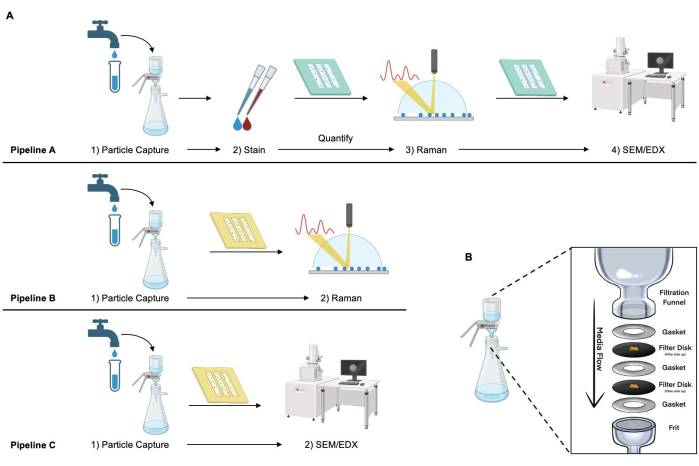
Figure 1: SNAP pipelines. (A) Schematics of SNAP pipelines, characterizing the same particles on the same nanomembrane via a series of different analytical techniques. Pipeline A) demonstrates 1) Captured particles of interest from drinking water samples via vacuum filtration are 2) stained with Nile Red and Trypan Blue for differentiation of synthetic versus non-synthetic polymeric particles, respectively, followed by 3) particle identification via Raman spectroscopy, and 4) SEM/EDX to characterize particle morphology and elemental identification. Pipeline B) demonstrates 1) Particle capture onto Au-SiN followed by 2) Raman spectroscopy. Pipeline C) demonstrates 1) Particle capture onto Au-SiN followed by SEM/EDX. (B) Schematic of the filter disk and silicone gasket in the filtration setup in the vacuum apparatus, depicting the sequential filtration through a 20 µm MPSN, then 8.0 µm MSSN nanomembrane, separated by silicone gaskets. Abbreviations: SNAP = Silicon Nanomembrane Analysis Pipeline; SEM = scanning electron microscopy; EDX = energy-dispersive X-ray spectroscopy; MPSN = microporous Silicon nitride. Please click here to view a larger version of this figure.

Figure 2: Drinking water sample collection sources. A regional map published by the Monroe County Water Authority depicting the locations from which each of the four drinking water samples were collected in the Greater Rochester, NY, region. Samples originated from different surface water sources: Lake Ontario (blue), Hemlock Lake (green), both Hemlock Lake and Lake Ontario (yellow), and Canandaigua Lake (purple). Please click here to view a larger version of this figure.

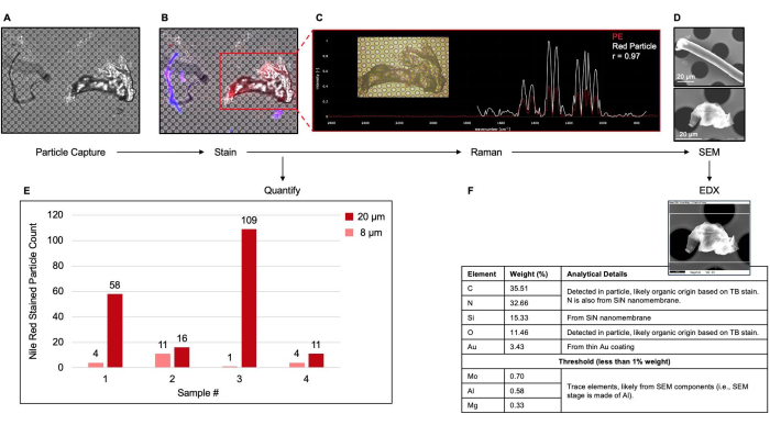
Figure 3: Summary of analyses from SNAP Pipeline A performed on particles captured from drinking water samples. (A) Greyscale image of captured particles from one representative drinking water sample on a 20 µm cut-off SiN. (B) False colored overlay image of counterstained particles to represent Nile Red (false-colored red particles) and Trypan Blue (false-colored blue particles). (C) Reference (red) and collected (white) Raman spectra identifying a Nile Red-stained particle as polyethylene with Pearson's r value of 0.97, with representative image of the particle analyzed. (D) Electron micrograph of two different particle types demonstrating particle morphology analysis of a fiber (top panel) and fragment (bottom panel), both taking up the Trypan Blue stain. (E) Quantification of Nile Red-stained particles sequentially captured onto both 20 µm and 8 µm cut-off nanomembranes. (F) Summarized EDX elemental analysis of a randomly selected fragment and analytical details of the results with representative SEM image of the particle analyzed. Abbreviations: SNAP = Silicon Nanomembrane Analysis Pipeline; SEM = scanning electron microscopy; EDX = energy-dispersive X-ray spectroscopy. Please click here to view a larger version of this figure.

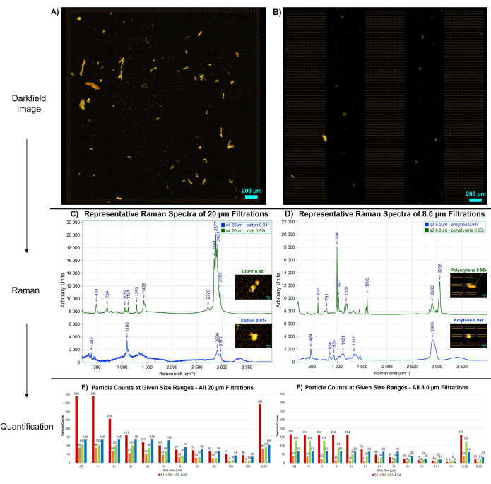
Figure 4: Summary of analyses from SNAP Pipeline B performed on particles captured from drinking water samples. Raman spectral analysis of three randomized particles from four household drinking water samples captured on 20 µm MPSN and 8.0 µm MSSN Au-SiN filter disks. Representative darkfield images of the total active membrane area for the 20 µm and 8 µm Au-SiN are respectively shown in A and B. Particles appear yellow in this imaging mode while the background remains dark, allowing for ease of automated particle counting. Representative Raman spectra of synthetic and non-synthetic particles on (C) 20 µm and (D) 8.0 µm Au-SiN. Total particle counts for (E) 20 µm and (F) 8.0 µm Au-SiN are binned by size ranges determined by the automated particle finding software. Abbreviations: SNAP = Silicon Nanomembrane Analysis Pipeline; SEM = scanning electron microscopy; EDX = energy-dispersive X-ray spectroscopy; MPSN = microporous Silicon nitride; MSSN = microslit Silicon nitride. Please click here to view a larger version of this figure.

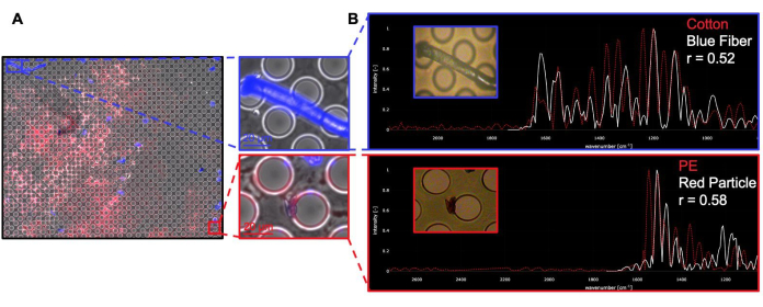
Figure 5: Suboptimal fluorescence Imaging and Raman spectroscopy results. (A) A suboptimal fluorescence image of stained particles (left panel), where the membrane retained the Nile Red stain, likely from under-rinsing. Two particles, a Trypan Blue-stained fiber and a Nile Red-stained fragment (right panel), were selected for Raman spectroscopy. (B) Suboptimal Raman spectroscopy results where the Pearson's coefficient (r) is less than 70 % (r < 0.70). Please click here to view a larger version of this figure.

Supplemental Table S1: Properties of silicon nanomembranes within filter disks. Depicted in this table are the properties of the membranes within the SiN filter disks, including the minimum pore size, the percent porosity, the thickness of the membranes with and without Au coating, the active area of the membrane, and the gas permeance through the membrane with positive pressure applied at a set constant pressure. Cut-off (i.e., pore size), porosity, thickness, and membrane area determined by measuring features on SEM images. Gas permeance data are reported as mean ± standard deviation (n = 10) for N 2 positive pressure applied at 103.42 kPa. Abbreviations: Au = Gold; Si_x N_y = Non-stoichiometric Silicon Nitride. Please click here to download this File.

Supplemental Table S2: ParticleFinder particle counts and parameters. Whole membrane area image mosaics were taken of each sample, and each image mosaic was analyzed to collect total particle counts. Depicted in this table are the parameters used and in what order to determine total particle counts for each sample image, and particle counts at given size fractions. Parameters vary from sample to sample given the type, quantity, and shape of particles, as well as the specific reflectivity of each membrane during imaging. The data from this table is visualized in Figure 4. Please click here to download this File.

Discussion

Microplastic pollution mitigation is a growing subject of concern; and the first step of mitigation is to identify the presence of contamination. A streamlined method of capture and immediate analysis is crucial to saving investigators time and preserving sensitive sample metrics. This report describes flexible workflows based on variations of our developed SNAP methods for the analysis of such MPs in liquid samples, utilizing a single substrate for all analyses conducted. The sample must be vacuum filtered such that the particles are captured and isolated onto a Silicon nanomembrane housed inside a filter disk. Sufficient mitigation of background contamination is critical for meaningful results. Any contaminating particles on the dispensing syringe or glass vacuum funnel during filtration may contaminate the sample and be concurrently captured, so following the Section 1 quality control protocols diligently is crucial for accurate outcomes. Media-only controls are recommended to inform investigators of background contamination specific to individual processes and laboratory conditions. The protocol described herein relies on vacuum filtration of a liquid sample, as well as capturing and isolating particles from the sample on two different cut-off SiN filter disks. For all pipelines, particle capture and isolation must precede other methods, but all other identification methods can be done in the order most suitable for the investigator.

Two fluorescent microscopes were utilized for this study to demonstrate repeatability of results across instruments. Instructional steps specifically detail the use of an Olympus BX61 for fluorescent microscopy due to the predominance of its use and was operated per instrument instructions utilizing brightfield for grayscale imaging, TRITC channel (Ex. ~543 nm; Em. ~593 nm) for NR-stained particle imaging, and Cy5 channel (Ex. ~649 nm; Em. ~667 nm) for TB-stained particle imaging, as applicable. To display the results of the staining, we recommend constructing an overlay of the channel images (we use FIJI/ImageJ for image processing, subsequently referred to as the image analysis platform), at a resolution of 2,048 x 2,040 pixels and a 16-bit depth. Whole nanomembrane images can be displayed as in Figure 4A,B or as selected regions of interest as shown in Figure 3A,B.

Nile Red is commonly used to stain synthetic polymer MPs but can stain non-synthetic polymers from biological sources due to its lipophilic and hydrophobic nature, potentially introducing false positives that distort MP quantification results^24,25,26. A Trypan Blue counterstaining step, as outlined in protocol section 3, is recommended to aid in the differentiation of false-positive events but is not an exhaustive solution and should be paired with additional analysis metrics to confirm results. Nile Red fluorescence of particles is a concern with Raman spectroscopy analysis as it may significantly increase the background signal. In this study, however, we counterstained polymers with Nile Red and Trypan Blue prior to Raman spectroscopy with an 830 nm laser, and little noise was observed, as shown in Figure 3.

Some wavelengths of lasers suitable for Raman spectroscopy are not able to ignore fluorescence from stained particles, such as a 532 nm laser, and therefore may introduce significant difficulty in correctly estimating the composition of the particle of interest. Metal coating the particles after capture is useful for enhancing the contrast during SEM imaging but is incompatible with any subsequent spectroscopic or fluorescent analysis. Make a note of all desired measurements prior to experimental setup to ensure that the process flow and coating types are taken properly into account. The Au-SiN filter disks can be utilized for all the mentioned analyses where transmission microscopy is not crucial to the workflow, or when Raman or IR spectroscopy is used.

The methods shown here, as well as the nanomembranes used to capture and isolate particles of interest, can be modified to suit individual investigators' needs. The nanomembranes are suitable for a number of spectroscopic analyses, and the investigator may swap the media being filtered for another sample media of interest, including but not limited to digested animal tissues²⁷, injectable pharmaceuticals, and oil samples. Two Raman spectroscopy instruments were utilized for this study, and instructional steps specifically detail the use of a Horiba XploRA Plus Raman instrument, which collected and processed all the data shown in Figure 4. It is also important to acknowledge the size limit of detection for each Raman microscope, to ensure the particles of interest can be suitably analyzed with the spot size of the instrument's lasers. To display particle identification results with Raman, the reference and sample spectra, plus an image of the analyzed particle, can be shown as in Figure 3C and Figure 4C.

Protocol section 6 details instructions for particle identification using an open-source spectral library. The planarized capture of particles onto a uniformly flat membrane, as well as the membrane's regular array of pores, enables predictable, automated imaging. Both the 400 nm or 1,000 nm thicknesses of the SiN and their Silicon nitride composition endow them with excellent optical transparency but may also return an intense Silicon peak in some spectroscopic instrument parameters. Care should be taken when utilizing bare, non-metal-coated SiN with Raman analysis. The Si peak may function as a calibration signal, but the intensity of the peak may also mask the signals of lower-intensity spectra in the same wavenumber region as the Si's signal. Such Si peaks were not observed when using the 830 nm laser in this study.

The ultrathin nature of the SiN (400 nm- or 1,000 nm-thick) and Au-SiN (520 nm- or 1,120-nm thick) used here endowed them with their excellent filtration, optical, and spectroscopic properties. However, these membranes must be protected from physical damage, such as by excessive differential pressure (i.e., ≥-206 kPa), direct touching by tweezers or fingers, or by improper gasket placement. The filter disk housing the membranes protects them and enables ease of handling under normal usage. When manipulating the filter disks, touch only the black outer ring, and never the active membrane area. Although not quantitatively reported here, the collection of captured particles onto a small amount of membrane surface area (3 x 3 mm for 20 µm and 3 x 0.7 x 3 mm for 8.0 µm cut-off membranes, respectively) potentially lowers total sample analysis time, by reducing the time needed to find and analyze particles of interest. This "concentration factor" is worthy of future exploration and may offer a unique benefit of SiN filter disks for investigators. In combination with their higher surface area-normalized flow rates versus other widely used membranes for MP characterization¹⁵, automated particle imaging routines that need only image a relatively smaller area of uniformly flat and in-focus SiN may further reduce total analysis times. However, any benefits related to the hypothesized concentration factor still need to be empirically demonstrated by comparing total processing times (from filtration to image analysis) on conventional and SiN filter disks.

We heuristically demonstrated the utility of the SNAP variations on local tap water samples. The protocol described here focuses on MP capture from drinking water sources around Rochester, NY. Sample collection proceeded as follows: for each sample collection, at least one liter of water was run through the faucet before collection started. New, sealed polypropylene bottles were taken to the running faucet and opened directly before collection. Bottles were not rinsed with drinking water before collection proceeded. Each sample consisted of two 500 mL bottles collected, one directly after the other. Each water sample came from a distinct household's pipe system, and the pipe material was not consistent throughout the sampling. Variables like the amount of recent water usage, time of collection, age of pipes, and the age of the home from which the sample came could not be controlled in this study. This was not a validated sample collection protocol. Each investigator should develop and validate their own collection procedures. However, for the sake of complete disclosure of methods, the above description is included. The filter disks allow repeated analysis on the same substrate for a number of analytical methods. No subsampling or multiple samples are needed outside of standard trial replicates. Eliminating the need for subsampling and multiple samples increases confidence in capturing information on low abundance targets. In addition to the enabling of multi-modal analysis methods, the SiN filter disks provide a distinct advantage over other analogous filtration medias due to the time-saving quality of a faster filtration rate per unit area¹⁵.

Materials

List of materials used in this article

Name	Company	Catalog Number	Comments
1 L Glass beaker	Pyrex	1000-1L
1 L Glass vacuum collection flask	Millipore Sigma	Z290459-1EA
100% cotton lab coat	Landau	LA-3172
100 mL glass filtration funnel	Advantec	311000	https://www.sterlitech.com/glass-filter-holder-311000.html
99% isopropyl alcohol	Fisher Scientific	A416-20
APEX EDS	EDAX		EDX software used to perform EDX analysis on captured particles.
Denton Prep Sputtering System	Denton Vacuum	DESK II : 293618089	Gold coating system
FIJI, image analysis platform	ImageJ	V 1.54F	FIJI (FIJI is just ImageJ) - a distribution of ImageJ
Glass screw-cap bottle	Corning	1395-250
Kimwipes	Kimtech	06-666-11C
LabSpec6	Horiba Scientific		Horiba Raman software containing ParticleFinder and ViewSharp
Laminar flow hood	Air Science	VLF-72A
Microscope	Olympus  / Nikon	BX61 / Ti2e	Any microscope with suitable fluorescence can be utilized for optical microscopy.
MPSN SiN filters	SiMPore Inc.	FD25-8.0-Au; FD25-8.0-NC FD25-20.0-Au, FD25-20.0-NC
Monoject 60 mL syringes	Coviden	8881560265
Nile Red powder	TCI	N0659
Nitrile Gloves	Ansell Microflex	19-167-17
OpenSpecy	openanalysis.org		Open source, spectral library
Oven	VWR	1310	Gravity Convection Utility Oven
P20 Pipette	Brandtech	705872
Pipette tip	Premium Vials	GS 151140R
Pourous support frit	Advantec	311000	Part of bundle
Raman instrument	Horiba	Xplora PLUS
Rubber stopper	Advantec	311000	Part of bundle
SEM instrument	Ziess	Auriga	Auriga Series, Modular Crossbeam workstation
Silicone gaskets	SiMPore	GASKET-25-R	Clear-cast PDMS gaskets, 0.8 mm thick
Silicone Roller	Sanyue	(ASIN: B07XDTNPS3)	Silicone roller -  8 x 5 x 2 inches
SmartSEM	Zeiss	V8	SEM software used to operate the Zeiss Auriga
Spray bottle	Uline	S-7273
Syringe filters	Thermo Scientific	CH2225-PES	0.22 µm luer lock syringe filters, 25 mm
Syringe pump	New Era Pump Systems, Inc.	NE-1000	Optional, but reccomended
Trypan Blue - 0.4%	Millipore Sigma	T8154-20ML
Tweezers	SiMPore	K6TWZR
Vacuum pump	Welch	847-676-8800
Vacuum tubing	Grainger	ZUSA-HT-4037

References

- Simon, M., Van Alst, N., Vollertsen, J. Quantification of microplastic mass and removal rates at wastewater treatment plants applying focal plane array (fpa)-based fourier transform infrared (ft-ir) imaging. Water Res. 142, 1-9 (2018).
- Da Costa Filho, P. A., et al. Detection and characterization of small-sized microplastics (≥ 5 µm) in milk products. Sci Rep. 11 (1), 24046(2021).
- Koelmans, A. A., et al. Microplastics in freshwaters and drinking water: Critical review and assessment of data quality. Water Res. 155, 410-422 (2019).
- Fendall, L. S., Sewell, M. A. Contributing to marine pollution by washing your face: Microplastics in facial cleansers. Mar Pollut Bull. 58 (8), 1225-1228 (2009).
- Kwon, J. -H., et al. Microplastics in food: A review on analytical methods and challenges. Int J Env Res Public Health. 17 (18), 6710(2020).
- Mahon, A. M., et al. Microplastics in sewage sludge: Effects of treatment. Environ Sci Technol. 51 (2), 810-818 (2017).
- Hidalgo-Ruz, V., Gutow, L., Thompson, R. C., Thiel, M. Microplastics in the marine environment: A review of the methods used for identification and quantification. Environ Sci Technol. 46 (6), 3060-3075 (2012).
- Ragusa, A., et al. Plasticenta: First evidence of microplastics in human placenta. Environ Int. 146, 106274(2021).
- Schwabl, P., et al. Detection of various microplastics in human stool. Ann Intern Med. 171 (7), 453-457 (2019).
- Leslie, H. A., et al. Discovery and quantification of plastic particle pollution in human blood. Environ Int. 163, 107199(2022).
- De Frond, H., et al. Monitoring microplastics in drinking water: An interlaboratory study to inform effective methods for quantifying and characterizing microplastics. Chemosphere. 298, 134282(2022).
- Nutrition and Food Safety (NFS), Standards & Scientific Advice on Food Nutrition (SSA). Dietary and inhalation exposure to nano-and microplastic particles and potential implications for human health. , https://www.who.int/publications/i/item/9789240054608 (2022).
- Fries, E., et al. Identification of polymer types and additives in marine microplastic particles using pyrolysis-GC/MC and scanning electron microscopy. Environ Sci: Processes Impacts. 15 (10), 1949-1956 (2013).
- Primpke, S., et al. Critical assessment of analytical methods for the harmonized and cost-efficient analysis of microplastics. Appl Spectrosc. 74 (9), 1012-1047 (2020).
- Carter, J., et al. Comparative evaluation of filtration and imaging properties of analytical filters for microplastic capture and analysis. Chemosphere. 332, 138811(2023).
- Van Mourik, L., et al. STOTEN's minimum requirements for measurement of plastics in environmental samples. Sci Total Environ. 912, 168465(2024).
- Käppler, A., et al. Analysis of environmental microplastics by vibrational microspectroscopy: FTIR, Raman or both. Anal Bioanal Chem. 408, 8377-8391 (2016).
- Mikoliunaite, L., et al. The substrate matters in the Raman spectroscopy analysis of cells. Sci Rep. 5 (1), 13150(2015).
- Madejski, G. R., et al. Silicon nanomembrane filtration and imaging for the evaluation of microplastic entrainment along a municipal water delivery route. Sustainability. 12 (24), 10655(2020).
- Romanick, S. S., et al. Assessment of household settled dust via silicon nanomembrane analysis pipeline (SNAP). Environ Technol Innov. 38, 104106(2024).
- Cowger, W., et al. Microplastic spectral classification needs an open source community: Open specy to the rescue. Anal Chem. 93 (21), 7543-7548 (2021).
- Kooi, M., Koelmans, A. A. Simplifying microplastic via continuous probability distributions for size, shape, and density. Env Sci Technol Lett. 6 (9), 511-564 (2019).
- SpectraBase. , John Wiley & Sons, Inc. SpectraBase. https://spectrabase.com/spectrum/1uoQJ4M5hxj (2025).
- Erni-Cassola, G., Gibson, M. I., Thompson, R. C., Christie-Oleza, J. A. Lost but found with nile red: A novel method for detecting and quantifying small microplastics (1 mm to 20 µm) in environmental samples. Environ Sci Technol. 51 (23), 13641-13648 (2017).
- Shim, W. J., Song, Y. K., Hong, S. H., Jang, M. Identification and quantification of microplastics using Nile Red staining. Mar Pollut Bull. 113 (1-2), 469-476 (2016).
- Greenspan, P., Mayer, E. P., Fowler, S. D. Nile red: A selective fluorescent stain for intracellular lipid droplets. J Cell Biol. 100 (3), 965-973 (1985).
- Cai, B., Andino, F. D. J., Mcgrath, J. L., Romanick, S. S., Robert, J. Ingestion of polyethylene terephthalate microplastic water contaminants by Xenopus laevis tadpoles negatively affects their resistance to ranavirus infection and antiviral immunity. Environ Pollut. 356, 124340(2024).
Reprints and Permissions