Transient Optical Clearing Using Absorbing Molecules for Ex Vivo and In Vivo Imaging

Summary

Optical clearing techniques, such as absorbing molecules solutions, reduce light scattering temporarily to enhance biological imaging and offer biocompatible, reversible in vivo imaging strategies for deeply embedded organs. This protocol presents detailed experimental procedures as well as advanced image processing to achieve high-quality, dynamic imaging for real-time dynamics in living animals.

Abstract

Dynamic imaging is a foundational tool in biology and medicine, but it is limited by light scattering in live tissues caused by refractive index mismatches, which reduces penetration depth and resolution in biological tissues. Previous work introduced a novel approach to achieve optical transparency in live animals by utilizing strongly absorbing molecules. When these absorbing molecules, such as Tartrazine, an FDA-approved dye commonly used in foods, dissolve in water, they modify the refractive index of the aqueous medium through Kramers-Kronig relations. This modulation allows reduction of the refractive index mismatch between separate components in tissue with distinct refractive indices, thus mitigating scattering. This article reports the detailed methodology of the tissue clearing technique using a Tartrazine-based aqueous solution, applied to both ex vivo and in vivo samples. This approach reversibly renders live mouse bodies transparent in the visible spectrum, enabling clearer and deeper imaging of internal processes and structures. An advanced image processing algorithm was then used to improve the contrast and segmentation of organs of interest. Additionally, high transparency in ex vivo samples, such as chicken breast, treated with Tartrazine-based solution, is shown. This method offers a versatile and accessible approach to enhance imaging capabilities across various modalities and paves the way for advancement in the understanding of complex biological systems.

Introduction

Biological imaging has long been challenged by the scattering of light, which obscures structures of interest¹. Optical clearing techniques aim to reduce light scattering and enhance visual clarity, enabling the visualization of previously hidden structures². The development of these techniques has led to a diverse array of methods designed to improve optical imaging of ex vivo biological tissues, even whole animals, without physical dissection of the samples³. However, the development of similar techniques for in vivo applications has been challenging. Techniques such as CLARITY Clear Lipid-exchanged Acrylamide-hybridized Rigid Imaging / Immunostaining / in situ-hybridization-compatible Tissue hYdrogel), offer high-resolution imaging but lack reversibility, making them unsuitable for live animal studies⁴. Constantini et al. have shown slower progress in in vivo imaging compared to ex vivo imaging clarity, which is due to the complexity of maintaining tissue viability while avoiding toxic levels of agents needed for tissue transparency⁵. Genina emphasizes the future of optical tissue clearing as reliant on non-invasive and reversible methods⁶. Recent studies have demonstrated the effectiveness of water-soluble absorbing dyes for in vivo optical clearing. For example, Miller et al. showed that topically applying Tartrazine significantly enhanced imaging depth in both OCT and photoacoustic microscopy (PAM) of live mouse skin, by reducing scattering and increasing the refractive index of interstitial tissue components⁷. Jia et al. used a 15% w/w Tartrazine solution to enhance in vivo PAM imaging of mouse ear and abdominal tissue, revealing fine microvascular structures with subcellular resolution that were otherwise obscured⁸. Zuo et al. further demonstrated brain imaging through intact scalp and skull in live mice using 0.6 M Tartrazine, achieving four times higher signal intensity and 3.5 times improved resolution compared to untreated tissue⁹. In another application, Narawane et al. enabled deep transscleral OCT imaging in porcine eyes by applying Tartrazine, achieving clear visualization of the suprachoroidal space, which was previously inaccessible due to strong scleral scattering¹⁰. Although ex vivo tissue clearing methods like CLARITY and iDISCO (Immunolabeling-enabled three-dimensional imaging of solvent-cleared organs) achieve high optical transparency and subcellular resolution through lipid removal or solvent-based clearing, they are often unsuitable for in vivo imaging with live animals^4,11,12. This limitation affects dynamic imaging, which is crucial for biomedical imaging of dynamic processes inside living animals, such as disease development and therapeutics.

Absorbing molecules with high aqueous solubility and distinct absorption band shapes, such as Tartrazine, a food-grade dye, offer promising advantages for achieving optical transparency in living animals¹³. By specifically introducing Tartrazine, the tissue selectively absorbs ultraviolet and blue wavelengths due to the dye's unique spectral characteristics, resulting in a modified refractive index profile that reduces scattering at longer wavelengths. This counterintuitive optical tissue clearing technique is optimized for in vivo imaging, and the Kramers-Kronig relations provide a scientific foundation for the observed transparency when using strongly absorbing molecules like Tartrazine^14,15. For in vivo imaging, Tartrazine is combined with heated agarose particles and water to create a cohesive solution that adheres to skin better. The water-soluble nature of Tartrazine also facilitates easy removal of the dye-based solution from live animals, reducing potential effects of extended exposure to dye solutions. Additionally, the method has been adapted for various biomedical applications to improve the imaging depth, resolution, as well as sensitivity, including optical coherence tomography^7,16 and photoacoustic imaging^7,9, demonstrating its potential for the broader biomedical imaging community.

With the growing interest in the application of absorbing molecules in biomedical imaging^17,18, the protocol presents a detailed procedure of utilizing food dye for ex vivo and in vivo applications, along with image processing and reversible in vivo imaging. This protocol is applied to chicken breast tissue to demonstrate ex vivo transparency and is then modified for in vivo head and abdominal imaging of mice, showing reversibility. A solution applied to mouse skin in vivo creates temporary, reversible transparency without harming the skin or tissue integrity. This technique can be integrated with an image processing pipeline, including denoising, to create an optimized imaging protocol for in vivo optical imaging of internal organs. When combined, these techniques enable better non-invasive, longitudinal imaging for real-time observations of biological processes. The use of safer agents that demonstrate reversibility overcomes previous limitations and provides a more suitable method for dynamic biological imaging.

Protocol

All animal experiments conducted were approved by The University of Texas at Dallas' Institutional Animal Care and Use Committee (IACUC) in accordance with the NIH Guide for the Care and Use of Laboratory Animals. The reagents and the equipment used are listed in the Table of Materials. Image processing code is available at Github: https://github.com/ou-group-utd/JoVE-2025-Image-Processing

1. Tartrazine solution preparation

1. For ex vivo samples
   1. To prepare dye solutions, calculate the required mass of dye powder (Tartrazine) to prepare the desired volume of the solution. Use the formula:
      Mass (g) = Molarity (M) × Molecular Weight (g/mol) × Volume (L)
      NOTE: To calibrate actual molarity, measure the absorbance of prepared solutions using a UV-VIS spectrometer and apply the Beer-Lambert Law¹⁹.
      ​CAUTION: Use an analytical balance to weigh the precise amount of the powder. Wear appropriate PPE (personal protective equipment), including a lab coat, gloves, and safety goggles, when working with dye powders. Avoid inhalation or skin contact.
   2. Transfer the dye powder to a clean glass vial and add the required volume of deionized (DI) water using a volumetric pipette to ensure volumetric precision.
   3. If the powder does not fully dissolve at room temperature, place the glass vial in a laboratory oven or furnace preheated to 40 °C and heat for 10 min or until powder is completely dissolved (Figure 1A).
      NOTE: Low molarity solutions are completely soluble at room temperature and remain in liquid form, while high concentration (>0.37 M) solutions require heating.
      CAUTION: Excessive heating will evaporate water and alter the actual concentration of the solution.
   4. Stir on vortex mixer for 30 s to 1 min to ensure complete dissolution.
   5. To prepare a 0.65 M solution, dissolve 427.5 mg of Tartrazine powder in 1 mL of DI water¹⁹. For other concentrations, refer to Table 1.
      NOTE: Dispose of unused dye solutions and contaminated materials according to standard chemical waste disposal procedures.
2. For in vivo samples
   1. Calculate the required mass of low-melting temperature agarose microparticles and Tartrazine to prepare a 0.65 M concentration with 0.4% (4 mg/mL) agarose hydrogel solution.
      NOTE: Follow standard safety precautions as described in step 1.1.1 when handling all reagents.
   2. Transfer the weighted powders into a clean glass vial. Add DI water using a volumetric pipette.
   3. Place the vial in a laboratory oven or furnace preheated to 75 °C for approximately 10-15 min or until the agarose particles are completely dissolved.
   4. Occasionally mix using a vortex mixer during the heating process for uniform dissolution.
   5. Allow the solution to cool to room temperature before use. If it solidifies into gel form, use the vortex mixer for 30 s to re-liquefy it.
   6. To prepare a 0.65 M hydrogel solution, dissolve 427.5 mg of Tartrazine powder and 4 mg of agarose in 1 mL of DI water. To prepare solutions of other concentrations, maintain the agarose concentration at 0.4% (4 mg/mL) and refer to Table 1 for the corresponding Tartrazine mass¹⁷.

2. Optical clearing of ex vivo tissues

1. Sample preparation
   1. To prepare ex vivo tissue, slice chicken breast tissue to the desired thickness parallel to the collagen fibers.
   2. Clean the sliced tissue gently with water.
   3. Measure thickness by placing the tissue between two clean microscope slides. Gently press the slides together and use a Vernier caliper to measure the distance between the slides at the center of the tissue.
   4. Soak the tissue in the dye solution.
      CAUTION: Make sure that the volume of the solution is more than the sample volume and that the tissue is completely submerged.
   5. Place the container on an orbital shaker and shake at 100 revolutions per minute for 10 min.
   6. Let the tissue stay in the solution for 60 min at room temperature for low concentrations ≤0.4 M and at 40 °C for higher concentrations >0.4 M.
2. Imaging
   1. Remove the tissue from the dye solution using clean forceps.
   2. Place the sample between two transparent glass slides and capture the images using a digital or scientific camera with appropriate resolution and magnification settings.
   3. Conduct the imaging process in a controlled light environment to minimize external light interference.
   4. Repeat the imaging process for tissue samples with different thicknesses and dye solution concentrations (Figure 2B).
      NOTE: Use an LED light source for back illumination. However, it works in the exact same way for a top illumination light source as well.
3. Optical transmission measurements
   1. To measure the optical transmission, sandwich the chicken tissue between two transparent glass slides and measure the transmission using a UV-Visible-NIR Spectrometer (Figure 2C).
   2. Ensure that the system is baselined properly, and the light beam passes through the same region of the tissue before and after treating it with dye solutions to maintain consistency.
      NOTE: Record the transmission spectra across a 400 nm to 2000 nm wavelength range, using a medium scan speed and a data interval of 1.0 nm. The full spectral scan takes approximately 5 min per sample.

3. Optical transparency in live animals

1. Animal preparation
   1. Before the experiment, measure the animal's weight and note down the general activity level to establish a physiological baseline.
   2. Use a heating pad with the temperature set to 37 °C to maintain the animal's body temperature during the experiment.
      CAUTION: Continuously monitor the animal to prevent overheating.
   3. Administer anesthesia in accordance with institutionally approved protocols appropriate for abdominal and brain imaging.
   4. For inhalation anesthesia, induce with isoflurane at 1.5%-3% and flow rate 0.8 L/min for approximately 5 min before the imaging experiment and maintain it at 1%-2% throughout the experiment.
      CAUTION: Monitor the animal's breathing pattern and depth continuously. Use a well-ventilated area to minimize anesthetic exposure to personnel.
   5. For injectable anesthesia, prepare a cocktail containing Ketamine HCL (16 mg/mL) and Dexmedetomidine HCL 0.2 mg/mL. Dose according to animal weight and approved institutional protocols.
   6. Trim the fur using small animal clippers from the desired imaging area.
   7. Apply depilatory cream to the trimmed skin area for less than 60 s to remove residual hair. Immediately remove the cream and clean the skin using alcohol wipes to avoid skin irritation.
   8. If injectable anesthesia with alpha-2 agonists (e.g., dexmedetomidine or xylazine) is used, administer atipamezole as the reversal agent following the experiment. Monitor the animal during recovery and ensure it returns to normal breathing and mobility before returning to its home cage.
2. Procedure for making tissue transparent
   1. Prepare the imaging setup by placing a heating pad set to 37 °C beneath the animal to prevent hypothermia. Align the light source and camera to capture the images.
   2. Use a 0.65 M Tartrazine hydrogel solution mixed with 0.3%-0.4% agarose gel for application (step 1.2).
   3. Apply the solution to the skin (belly or head, depending on the nature of the experiment) using a dropper and allow it to sit for a few seconds to initiate absorption (Figure 3A).
   4. Gently scrub the area using a cotton swab for even distribution of the dye solution and facilitate dermal absorption.
   5. Massage the area gently with a clean cotton swab and apply more solution till the skin starts showing transparency and internal organs are visible. During absorption, the skin will first show the appearance of orange-red dots, which gradually merge into a uniform color. This color change is a key visual indicator of adequate dye penetration and onset of optical clearing.
      CAUTION: Ensure that the solution does not crystallize over the application area - crystallization can block skin passages, hindering the dye molecules' absorption in the skin, which is highly crucial to achieve transparency. Sufficient absorption of dye molecules turns skin's color to orange-red.
   6. Continue massaging the area gently until the skin starts showing transparency and internal organs become visible. This process typically takes approximately 3-5 min of massaging for a small area, but duration may vary depending on animal size and skin thickness.
   7. Capture images using the aligned camera. Adjust focus, exposure, and white balance to optimize image quality.
   8. Gently place a glass slide or cover slip on the skin to minimize shine and reduce reflection for better quality images.
      CAUTION: Handle all chemical solutions with proper personal protective equipment (lab coat, gloves, and eye protection), and dispose of used materials in accordance with the institution's chemical waste disposal protocols.

4. Increasing organ visibility with image processing

1. Image processing steps
   1. Python with OpenCV is used for image processing. Import OpenCV, numpy, matplotlib, and PyWavelets.
   2. Load and Normalize the original Image. Load the original high-bit-depth .tif image. If any pixel value exceeds 255, normalize all pixels to the range [0, 255].
   3. Crop the Region of Interest (ROI). Invoke OpenCV's ROI selector to draw a bounding box around the organ area. Proceed only using the cropped version for all subsequent steps.
      NOTE: Ensure that the bounding box tightly encloses the target area without cutting off any relevant structures.
   4. Split into LAB Channels. Convert the cropped color image to LAB color space and split into L(lightness), A, and B channels.
      NOTE: Images are being processed in color, so the lab color space was used with image processing techniques being applied only to the L channel, where pixel intensities are located.
   5. Analyze Pixel Intensity Distribution. Plot a histogram of the L channel to assess contrast and intensity spread.
      NOTE: Use the histogram to verify whether contrast enhancement is necessary and to guide parameter selection for contrast enhancement. You want your histogram to be spread across [0, 255].
   6. Apply CLAHE (Contrast Limited Adaptive Histogram Equalization) for local contrast enhancement. Create a CLAHE object with clipLimit = 5.0 and tileGridSize = (16,16). Execute CLAHE on the L channel and merge the CLAHE-enhanced L channel with the original A and B channels. Convert CLAHE from LAB to RGB for visualization if needed.
      NOTE: If the histogram shows over-amplified noise (spikes), adjust 'clipLimit' or 'tileGridSize' and reapply to achieve balanced local contrast.
   7. Denoise the contrast-enhanced image. Perform a 2-level discrete wavelet decomposition on the normalized CLAHE L channel (scaled [0, 1]) with a soft threshold of 0.1. Reconstruct the denoised L channel, scale back to [0, 255], and merge the denoised L channel with the original A and B channels. Display the original cropped color image versus the wavelet-denoised result.
      NOTE: Wavelet denoising reduces small fluctuations that might be misinterpreted as foreground in uniform regions.
   8. Segment organs of interests via Otsu's Adaptive Thresholding. Compute Otsu's threshold on the denoised L channel. Subtract a bias of 15 from the threshold to include low-intensity organ regions.
      1. Apply a binary threshold with the bias value to obtain a mask of the organ pixels. Merge the mask with the original A and B channels and convert to RGB for viewing.
         NOTE: The bias adjustment forces inclusion of organ regions beneath vessels. Re-tune bias if needed for a different dataset.
   9. Proceed to analysis as desired.

Results

Demonstration of optical transparency in ex vivo chicken breast tissue
To investigate light propagation through ex vivo tissue, we used sliced pieces of raw boneless chicken breast with thicknesses of 1.5 mm, 2.5 mm, and 3.5 mm (Figure 2B). The tissues were cut parallel to collagen fibers, ensuring consistent muscle fiber orientation. Images were taken using both a mesh grid pattern and "UT Dallas" logo underneath the tissue before and after treating with different solution concentrations (Figure 2B). To capture the images, a CMOS camera paired with a lens featuring a 3.5 mm focal length and f/1.4 aperture was used, and an LED light source was used for back illumination of the sample. The corresponding transmission data for each tissue was then measured using a UV-VIS-NIR spectrometer (Figure 2C).

The optical transparency of the tissue can be visualized by the naked eye and quantified with spectrometer measurements. For the untreated chicken tissues, the underlying patterns are completely invisible, and the transmission values in the visible region are approximately 2.4%, 1.7% and 1% for tissue thicknesses of 1.5 mm, 2.5 mm, and 3.5 mm, respectively. At 1064 nm wavelength, the transmission values are 8%, 5% and 1.8% for the same thicknesses. The solutions were prepared by dissolving the Tartrazine powder in deionized water. After the tissues were soaked in Tartrazine solutions of increasing concentrations, the dye molecules diffused throughout the extracellular matrix and cellular compartments, altering the refractive index of the interstitial medium¹³. This refractive index matching substantially reduces the light scattering within tissue, resulting in enhanced dynamic imaging and higher transmission in spectroscopic measurements. As the Tartrazine concentration increased from 0-0.65 M, the refractive index of dye solutions increased, and the transparency of the tissue substantially improved. For 0.65 M dye solution, the grid pattern and UT Dallas logo underneath the tissues become clearly visible, and transmission increased to 38.7%, 25%, and 21.7% in the visible spectrum for thicknesses of 1.5 mm, 2.5 mm, and 3.5 mm, respectively. At 1064 nm wavelength, the transmission values were 50%, 36.8% and 37.5% for the same samples.

Demonstration of optical transparency in living animals
For dynamic imaging in live animals, a dye solution with 0.65 M concentration was prepared, and 0.4% low-melting agarose was added to adjust the solution's viscosity and improve adherence to the skin. During the gut imaging, the animal was anesthetized using inhalation anesthesia, and the body temperature was maintained at 37 °C using a digitally controlled heating pad. Abdominal fur was removed by shaving and applying hair removal cream on the skin, following the process shown in Figure 3B, and then the topical application of 0.65 M dye solution. The Tartrazine solution was applied to the skin for 2 min and then gently massaged. Immediately, within a few minutes, the dye molecules diffuse into the extracellular matrix and superficial dermal layers. The diffusion of the dye molecules reduces the refractive index mismatch between low-index aqueous interstitial fluid and high-index lipid-rich structures, resulting in reduced scattering of incident light at tissue interfaces and cellular boundaries. As a result, the skin becomes visibly transparent in the visible spectrum for wavelengths longer than 550 nm, making it possible to visualize the deep-seated organs without surgically removing the skin (Figure 3B-E). For optical imaging of the brain vessels, the mouse was anesthetized using injectable anesthesia, and fur was removed before the application of the dye solution. The results demonstrate transparency of the scalp and visualization of cerebral blood vessels, validating the effectiveness of this technique for brain imaging (Figure 3F,G).

To demonstrate the reproducibility of the protocol, the transparency results obtained for three different mice are presented in Figure 3. Young adult female mice (3-4 weeks old, approximately 10-12 g) are used for abdominal imaging, including two different mouse lines, C57BL/6J (Figure 3C,F) and Chat-Cre x tdTomato (Figure 3E). The results obtained for all three mice show enhanced transparency of the skin and visualization of the internal organs after treatment with dye solution, validating this tissue-clearing approach. Results from mouse-1 are displayed in detail over multiple time points and reveal gradual transparency over the time of gel solution application while highlighting temporal progression and effectiveness of the method (Figure 3B,C). It is worth noting that even for mice of the same sex and similar ages, the arrangements and visual appearance of internal organs can vary between individuals, highlighting the unique advantage of chronic imaging of the same animal for developmental studies.

Reversibility
The optical tissue clearing approach used in this protocol is reversible, which gives this approach a significant advantage for in vivo applications. The optical transparency of the tissue can be reversed by simply rinsing and gently massaging the skin with water. In this case, the transparency effect disappears immediately, and the yellow coloration from the dye fades within a few minutes. If the tissue is not rinsed, the color gradually disappears over the course of a few hours due to passive diffusion. The image shown in Figure 3B, captured after 2 h of the abdominal experiment, indicates that transparency is temporary, and it can be fully reversed. Following reversal, the skin maintains a normal appearance, and the mice exhibit typical activity, and the hair on the treated skin regrows within several days (Figure 3C). This further confirms the safety and effectiveness of this approach for dynamic imaging in live animals, especially for potential chronic imaging applications of the same animals (Figure 4 and Table 2).

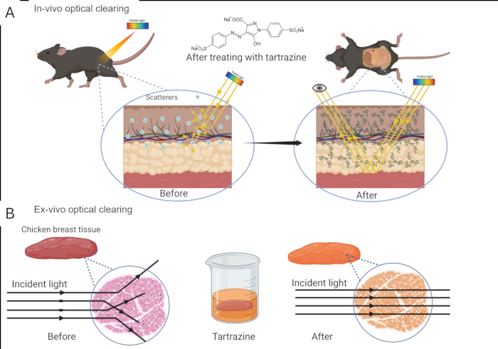
Figure 1: Schematic illustration of the in vivo (A) and ex vivo (B) optical clearing of tissue using absorbing molecule solutions. Please click here to view a larger version of this figure.

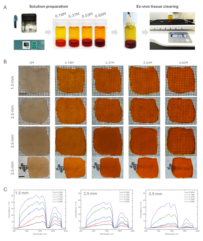
Figure 2: Procedure for optical clearing of ex vivo tissue. (A) Photographs of the solutions preparation and clearing processes of the ex vivo tissue. (B) Optical images of the chicken breast tissue with different thicknesses placed on top of a pattern. (C) Optical transmittance spectra of the chicken breast tissue with different thicknesses. Scale bars: 5 mm. Please click here to view a larger version of this figure.

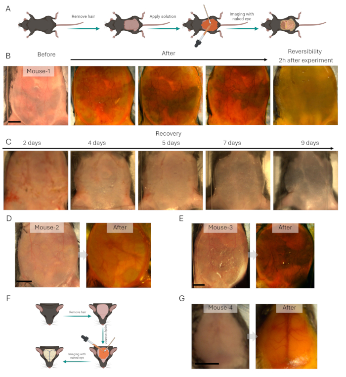
Figure 3: Procedure for optical clearing and imaging of animals. (A) Schematics illustrating the application of absorbing molecules on the mouse belly. (B) Temporal image series illustrates that the tissue becomes transparent and returns to opacity after the experiment. (C) Long-term monitoring of the tissue of the mice illustrating the recovery of the mice's belly. (D,E) Optical imaging results from two different animals. (F) Schematics illustrating the application of absorbing molecules on the mouse head. (G) Images showing the change of transparency of tissue for visualizing the vessels on the surface of the brain. Scale bars: 5 mm. Please click here to view a larger version of this figure.

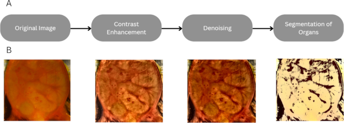
Figure 4: Image processing for improved visualization of organs. (A) Workflow showing the image processing steps from a raw image to segmented organ images. (B) Representative images showing each step after image processing. Please click here to view a larger version of this figure.

Tartrazine mass (mg) dissolved in 1 mL water	Relative percentage of Tartrazine in solution	Calibrated molecular concentration (M)
106.9	9.70%	0.18
213.7	17.60%	0.37
320.8	24.30%	0.53
426.6	29.90%	0.65

Table 1: Preparation recipe of Tartrazine solutions of different concentrations.

Image Processing Step	Library	Function (Code)
Import Libraries	OpenCV, numpy, matplotlib, PyWavelets	import cv2 import numpy as np import matplotlib.pyplot as plt import pywt import os
Loading the original .TIF image	cv2	color_image = cv2.imread(image_path, cv2.IMREAD_UNCHANGED)
Normalization if pixel values exceed 255	numpy & cv2	if color_image.max() > 255:     color_image = (color_image / color_image.max()) * 255 color_image = color_image.astype(np.uint8)
Display color image	matplotlib.pyplot & cv2	plt.imshow(cv2.cvtColor(color_image, cv2.COLOR_BGR2RGB)) plt.axis("off") plt.show()
Cropping (selecting ROI interactively)	cv2	roi = cv2.selectROI("Select Region", color_image, fromCenter=False, showCrosshair=True) x, y, w, h = roi cropped_color = color_image[y:y+h, x:x+w] cv2.destroyAllWindows()
Split LAB channels	cv2	lab_color = cv2.cvtColor(cropped_color, cv2.COLOR_BGR2LAB) l_channel, a_channel, b_channel = cv2.split(lab_color)
Analyzing pixel distribution (histogram of intensities)	matplotlib.pyplot	plt.figure(figsize=(8,6)) plt.hist(l_channel.ravel(), bins=256, range=[0,255], color='black', alpha=0.7) plt.title("Pixel Intensity Distribution") plt.xlabel("Intensity Value") plt.ylabel("Pixel Count") plt.grid() plt.show()
Applying CLAHE to spread pixel intensities	cv2	clahe = cv2.createCLAHE(clipLimit=5.0, tileGridSize=(16,16)) l_channel_clahe = clahe.apply(l_channel) lab_clahe = cv2.merge((l_channel_clahe, a_channel, b_channel)) cropped_color_clahe = cv2.cvtColor(lab_clahe, cv2.COLOR_LAB2RGB)
Plot CLAHE-enhanced image and histogram	matplotlib.pyplot	plt.figure(figsize=(15,5)) plt.subplot(1,2,1) plt.title("CLAHE Enhanced Image") plt.imshow(cropped_color_clahe) plt.axis("off") plt.subplot(1,2,2) plt.hist(l_channel_clahe.ravel(), bins=256, range=[0,255], color='black', alpha=0.7) plt.title("Pixel Distribution after CLAHE") plt.xlabel("Intensity Value") plt.ylabel("Pixel Count") plt.grid() plt.show()
Applying wavelet denoising to image	pywt, numpy & cv2	coeffs = pywt.wavedec2(np.float32(l_channel_clahe)/255.0, 'db1', level=2) coeffs_thresh = list(coeffs) for i in range(1, len(coeffs_thresh)):     coeffs_thresh[i] = tuple(pywt.threshold(subband, 0.1, mode='soft') for subband in coeffs_thresh[i]) l_wavelet = np.uint8(pywt.waverec2(coeffs_thresh, 'db1') * 255) lab_wavelet_denoised = cv2.merge((l_wavelet, a_channel, b_channel)) color_wavelet_denoised = cv2.cvtColor(lab_wavelet_denoised, cv2.COLOR_LAB2RGB)
Display original vs. wavelet-denoised image	matplotlib.pyplot & cv2	plt.figure(figsize=(12,6)) plt.subplot(1,2,1) plt.imshow(cv2.cvtColor(cropped_color, cv2.COLOR_BGR2RGB)) plt.title("Original Color Image") plt.axis("off") plt.subplot(1,2,2) plt.imshow(color_wavelet_denoised) plt.title("Wavelet Denoised Image") plt.axis("off") plt.show()
Thresholding for segmenting organs (Otsu’s method)	cv2	otsu_val, _ = cv2.threshold(l_wavelet, 0, 255, cv2.THRESH_BINARY_INV + cv2.THRESH_OTSU) bias_val = otsu_val - 15 _, otsu_adjusted = cv2.threshold(l_wavelet, bias_val, 255, cv2.THRESH_BINARY) otsu_segmented = cv2.cvtColor(cv2.merge((otsu_adjusted, a_channel, b_channel)), cv2.COLOR_LAB2RGB) plt.imshow(otsu_segmented) plt.axis("off") plt.show()

Table 2: Image processing steps, libraries, and scripts.

Discussion

This work presents a comprehensive and reproducible protocol method to achieve optical transparency in biological tissues utilizing absorbing molecules, specifically FDA-approved food dye Tartrazine (approved for use in food products, not in medical applications). This method effectively minimizes intrinsic scattering in tissue by altering the refractive index within the tissue's microenvironment, which enhances optical transparency. This study demonstrated the effectiveness of this method through both ex vivo and in vivo imaging. For ex vivo imaging, the effect of different concentrations of Tartrazine on chicken breast tissue was investigated with different thicknesses of the biological samples. The results indicate that an optimal concentration of Tartrazine can make chicken breast tissues transparent to the naked eye. The spectroscopic measurements of transmission further reveal that although incident light is almost completely absorbed below 550 nm, transmission of light through the tissue significantly increases for longer wavelengths of the visible spectrum and into the near infrared region. These wavelengths are commonly used in deep-tissue imaging, making this approach highly compatible with various imaging modalities. One critical parameter for successful ex vivo clearing is the dye concentration, which must balance maximizing optical transparency while avoiding saturation or crystallization. The current protocol relies on the passive diffusion of dye molecules into the tissue, which limits the applications to larger samples, since the diffusion time required is proportional to the square of the thickness of the samples².

For in vivo imaging, we have demonstrated this approach for abdominal and brain imaging in live animals. The application timing and massage duration are crucial steps, gentle massaging for 3-5 min ensures even distribution and adequate penetration. A visual cue, such as the skin turning orange-red, serves as an intermediate checkpoint indicating sufficient absorption. This innovative transient optical clearing technique has led to a new strategy for integrative biology research by enabling high-resolution, real-time imaging of dynamic anatomical and functional processes, such as organ regeneration and internal movement, within intact live tissues. Reversibility is another key advantage of the protocol. Once the dye solution is removed, the transparency effect reverses immediately upon washing, and the skin returns to normal appearance within hours. If left unwashed, the dye diffuses out passively over a few hours. No damage or irritation was observed post-application, and hair regrew normally on treated areas within days. This method is compatible with existing optical imaging modalities and contrast agents, non-invasive, and allows imaging at any location within the animal body without restricting animal behavior. Combined with other optical imaging techniques such as multiphoton-microscopy²⁰ and near-infrared imaging²¹, it can provide detailed insights into structural characterization, microenvironment, and cell phenotypes, facilitating studies on dynamic physiological processes and disease prevention. This protocol provides a time-efficient, accessible, and easily adoptable alternative to existing invasive or terminal optical clearing techniques. Its simplicity, reversibility, and compatibility with existing imaging tools make it a powerful method for high-resolution in vivo studies across various research domains, including developmental biology, neuroscience, oncology, and regenerative medicine.

Materials

List of materials used in this article

Name	Company	Catalog Number	Comments
Analytical Balance	HZK	FA220S
Animal anesthesia Machine	RWD life science co	TAIJI-IE	Inhalation Anesthetics
Atipamezole HCL injection 5 mg/mL	Covertus	82124	Injectable anesthesia
CMOS camera	Thor labs	CS165CU/M, Zelux
Dexmedetomidine HCL injection 5 mg/10 mL	Covertus	72960	Injectable anesthesia
Fiber Light Illuminator	RWD life science co	76301	Light source for top illumination
Glass slides	CravitySci	0303-2122	Super grade microscope slides
Homeothermic Blanket	RWD life science co	69027	Animal temperature controller
Image Processing	OpenCV	Python	Software
Insulin Syringe 0.5 mL 29 G	Comfort point	26028	Injectable anesthesia
Isoflurane	Covertus	SKU 029405	Inhalation Anesthetics
Ketmine HCL injection 100 mg/mL	Dechra	20042240	Injectable anesthesia
LED light source	GGE corp	TLB-01	Light source for top illumination
Lens	Thor labs	MVL4WA	3.5 mm focal length and f/1.4 aperture
Nair	Church & Dwight	L 1224	Hair removal Cream
PBS ph 7.4 (1x)	Gibco	2902869	Injectable anesthesia
Q-Tip	Puritan medical products company	806-wc hospital
SeaPlaque Agarose	Lonza	50101	Chemical
Tartrazine	MilliporeSigma	CAS number: 1934-21-0	Chemical
Transfer pipette	Fisherbrand	13-711-9AMMD
UV-VIS-NIR Spectrophotometer	Shimadzu	SolidSpec-3700i	Instrument
Vials	Qorpak	242633
Volumetric pipettes	Eppendorf research plus	3123000063	100-1000µL
Water Purification System	Avidity science	SOLO S	Instrument

References

- Yun, S. H., Kwok, S. J. J. Light in diagnosis, therapy and surgery. Nat Biomed Eng. 1 (1), 0008(2017).
- Tuchin, V. V. Optical clearing of tissues and blood. , SPIE Publications. (2005).
- Ertürk, A. Deep 3D histology powered by tissue clearing, omics and AI. Nat Methods. 21 (7), 1153-1165 (2024).
- Chung, K., et al. Structural and molecular interrogation of intact biological systems. Nature. 497 (7449), 332-337 (2013).
- Costantini, I., Cicchi, R., Silvestri, L., Vanzi, F., Pavone, F. S. In vivo and ex vivo optical clearing methods for biological tissues: Review. Biomed Opt Express. 10 (10), 5251-5267 (2019).
- Genina, E. A. Tissue optical clearing: State of the art and prospects. Diagnostics. 12 (7), 1534(2022).
- Miller, D. A., et al. Enhanced penetration depth in optical coherence tomography and photoacoustic microscopy in vivo enabled by absorbing dye molecules. Optica. 12 (1), 24-30 (2025).
- Jia, C., et al. Tartrazine-enabled optical clearing for in vivo optical resolution photoacoustic microscopy. Biomed Opt Express. 16 (6), 2504-2515 (2025).
- Zuo, T., Tao, C., Liu, X. Absorbing molecules as optical clearing agents improve the resolution and sensitivity of photoacoustic microscopy. Opt Lett. 50 (7), 2282-2285 (2025).
- Narawane, A., et al. Optical clearing with Tartrazine enables deep transscleral imaging with optical coherence tomography. J Biomed Photonics Eng. 29 (12), 120501(2024).
- Ueda, H. R., et al. Tissue clearing and its applications in neuroscience. Nat Rev Neurosci. 21 (2), 61-79 (2020).
- Mai, H., et al. Whole-body cellular mapping in mouse using standard IgG antibodies. Nat Biotechnol. 42, 617-627 (2024).
- Ou, Z., et al. Achieving optical transparency in live animals with absorbing molecules. Science. 385 (6713), eadm6869(2024).
- Sai, T., Saba, M., Dufresne, E. R., Steiner, U., Wilts, B. D. Designing refractive index fluids using the Kramers-Kronig relations. Faraday Discuss. 223, 136-144 (2020).
- Yu, T., Zhu, D. Strongly absorbing molecules make tissue transparent: A new insight for understanding tissue optical clearing. Light Sci Appl. 14 (1), 10(2025).
- Drexler, W., et al. Optical coherence tomography: Technology and applications. Drexler, W., Fujimoto, J. G. , Springer International Publishing. Cham. 277-318 (2015).
- Wang, F., Zhou, C. Transparent mice': Deep-tissue live imaging using food dyes. Commun Biol. 7 (1), 1307(2024).
- Yu, H., Liu, J. -B., Ma, Y. -S., Fu, D. Transparent live mice offer more possibilities for biomedical research. Innov Med. 2 (4), 100098(2024).
- Shabbir, M. W., Biswas, S., Kajla, R., Nadella, S., Ou, Z. Designing refractive index fluids of food dye for light propagation through scattering media. MRS Commun. , (2025).
- Scheele, C. L. G. J., et al. Multiphoton intravital microscopy of rodents. Nat Rev Methods Primers. 2 (1), 89(2022).
- Schmidt, E. L., et al. Near-infrared II fluorescence imaging. Nat Rev Methods Primers. 4 (1), 23(2024).
Reprints and Permissions