Dynamic clamp electrophysiology can establish causal links between neuronal firing deficits and ion channel dysfunction. We describe dynamic clamp methods and protocols in mouse cerebellar Purkinje neurons, noting useful resources and technical considerations. In a representative study, we add modeled sodium conductance to Tsc1-/- Purkinje neurons to rescue repetitive firing.
Method Article
Dynamic Clamp Methods to Investigate Impaired Neuronal Excitability Associated with Autism
In This Article
Summary
Abstract
Autism spectrum disorder (ASD) arises from a wide range of genetic and environmental factors. While numerous ASD-linked mutations disrupt synapse development or plasticity, an increasing number have been shown to alter the expression and functioning of voltage-gated ion channels, resulting in deficits in neuronal intrinsic excitability. Whole-cell voltage-clamp recordings can be used to characterize how ASD-related mutations affect ion channel function. However, these experiments fail to directly assess how an altered ionic conductance affects neuronal action potential firing. Dynamic clamp electrophysiology bridges this gap by enabling real-time injection of user-defined ionic conductances into living neurons. This allows causal testing of how changes in ion channel properties affect the electrical activity of a given cell type. In this methods article, we describe how to implement dynamic clamp electrophysiology in adult mouse Purkinje neurons recorded under physiological conditions in acutely prepared cerebellar brain slices. Purkinje neurons are a particularly relevant model for this work because they have an intrinsic capacity to fire repetitive, high-frequency (20-100 Hz) action potentials and are consistently implicated in ASD-related cerebellar circuit dysfunction. We focus on Tsc1, a gene whose loss-of-function mutations are among the most common monogenic causes of ASD. In mouse Purkinje neurons, Tsc1 deletion has also been linked to reduced voltage-gated sodium (Nav) channel expression. We utilize Markov kinetic state models to simulate and reproduce Purkinje neuron Nav conductance properties and go on to use dynamic clamp to directly assess how changes in the Nav conductance impact the intrinsic firing of intact cerebellar Purkinje neurons. We provide instructions and resources for modifying and tuning ionic conductance models. By integrating ionic conductance modeling, dynamic clamp, and conventional patch-clamp techniques, this approach provides a powerful and flexible framework for linking genetic perturbations to physiological outcomes in ASD-relevant neurons.
Introduction
Previous investigations into the molecular and cellular drivers of autism spectrum disorder (ASD) often emphasized synaptic dysfunction as central to the disorder's pathophysiology1,2. Numerous studies have demonstrated increased excitatory synapse density2,3,4, impaired synaptic pruning5, and alterations in postsynaptic density proteins6,7 in ASD models. However, recent work has shown that changes in intrinsic neuronal excitability are also drivers of ASD pathology. For instance, ASD transgenic mouse models and patient-derived cell lines have revealed impaired action potential generation in cerebellar Purkinje8,9,10 and cortical pyramidal neurons11, as well as attenuated dendritic excitability and synaptic integration in subclasses of cortical pyramidal neurons12. Channelopathies involving loss-of-function mutations in SCN2A, encoding the voltage-gated sodium (Nav) channel Nav1.2 pore-forming α subunit, is now a well-known monogenic cause of ASD13, and has been shown to cause deficits in the intrinsic excitability of various classes of central neurons14,15,16,17. As these types of investigations progress, it is important to establish causal links between pathogenic changes in ionic conductances and the effects of these changes on neuron and circuit function. Dynamic clamp electrophysiology provides an effective approach for this task. Sharp et al. (1992 and 1993)18,19, along with Robinson and Kawai (1993)20 initially described dynamic clamp methods in which a simulated non-linear ionic conductance, with or without voltage-dependent properties, is injected/added into living neurons, allowing investigators to assess in real-time how the properties or putative changes in a voltage-gated ionic conductance affect neuronal firing21,22.
The implementation of dynamic clamp experiments has been facilitated by several freely available software systems such as RTXI23, QuB24,25, and StdpC26; however, recent advancements have simplified dynamic clamp implementation with commercial plug-and-play systems that enable model conductances to be developed, modified, and applied on a single computer and within a single software package. Here, we provide protocols to perform dynamic clamp using a Sutter dPatch system27 and provide a sample investigation in which we test how the targeted deletion of tuberous sclerosis 1 (Tsc1)9, which is a prevalent locus of mutations for ASD28, affects the intrinsic firing of cerebellar Purkinje neurons as a result of changes in the expression of the voltage-gated sodium conductance8.
Protocol
All animal experiments were performed in accordance with protocols approved by the Miami University Institutional Animal Care and Use Committee guidelines (Protocol #1044). Experiments utilized male and female wild-type C57BL/6J mice and transgenic lines with a C57BL/6J strain background. For electrophysiological experiments, animals were aged 6-7 weeks. All recordings were taken from Purkinje neurons in lobules 5, 6, or 7 in the cerebellar vermis.
1. Setup and tissue preparation for Purkinje neuron patch-clamp experiments
- Prepare 1 L of artificial cerebral spinal fluid (ACSF) containing: 125 mM NaCl, 2.5 mM KCl, 1.25 mM NaH2PO4, 25 mM NaHCO3, 2 mM CaCl2, 1 mM MgCl2, and 25 mM dextrose at pH 7.4 (~300 mOsM/L). Also prepare 250 mL of 'cutting solution' containing: 240 mM sucrose, 2.5 mM KCl, 1.25 mM NaH2PO4, 0.5 mM CaCl2, and 7 mM MgCl2. Sparge (bubble) ACSF and cutting solutions with carbogen (95 % O2/ 5% CO2) gas for at least 20 minutes prior to use and continuously throughout all experiments.
- Prepare a brain slice holding chamber filled with ACSF for later use. Ensure that cerebellar slices (once added to the slice chamber) are submerged with both sides of the cerebellar slices exposed to ACSF. Accomplish this by placing submerged slices on a tightly stretched nylon mesh that is also submerged.
- Prepare the surgery station. Ready four pieces of tape that will be used to pin the anesthetized animal. In an ice-filled bucket or ice pan, place the bottom half of a Petri dish into the ice with the walls facing down and the Petri dish bottom facing up. Place a filter paper (≥ 3 cm2) on the Petri dish bottom and saturate with 2-3 mL of cutting solution.
NOTE: For the described experiments, a compresstome vibratome is used to slice 350 µM parasagittal cerebellar slices. With the compresstome, tissue for slicing is glued to a plastic specimen tube that fits through a surrounding thin metal tube. During slicing, the specimen tube is pushed through the metal tube, which remains fixed. After the tissue is glued to the specimen tube, the tissue is embedded in warmed 2% agarose. The blade of the compresstome is glued onto a fixed holder, which is attached to the arm of the vibratome. Other types of vibratomes do not require embedding tissue in warmed agarose, but should work similarly well for the described experiments. - Also, in the ice, place a single-edged razor blade and a small (10 mL) beaker filled with cutting solution. Keep a chilling block, which is used to rapidly cool the warmed agarose once it is added to the specimen tube, as well as a 30 mL syringe filled with cutting solution chilled on the ice. Ensure that the 30 mL syringe is connected to a 30-60 cm section of intravenous (IV) tubing (via Luer lock male taper) that is connected (at the terminating end) to a needle (≥ 26 G) with a Luer lock female base.
- Place the remaining cutting solution into a -80 °C freezer. Once this cutting solution becomes a slushed ice consistency (20-25 min), remove from the -80 °C freezer and place on ice.
- Anaesthetize a 5-8 week-old adult mouse with an intraperitoneal injection of 1 mL/kg animal weight of ketamine (10 mg/mL)/xylazine (0.25 mg/mL) cocktail.
- Make a 2% agarose solution by dissolving 0.5 g of agarose in 25 mL of cutting solution. After the animal is anesthetized (does not respond to toe pinch), heat the 2% agarose solution (~30 s in microwave) and transfer the warmed agarose solution to a 40 °C water bath.
NOTE: Steps numbered 1.8-1.18 must be completed with urgency and before the warmed agarose solidifies. - Pin the limbs of the animal to the surgery table with tape. Using scissors, open the thoracic cavity of the animal, ensuring that the lungs and abdominal organs are not cut. Use locking forceps or hemostats to hold the rib cage open, exposing the heart. To accomplish this, lock the forceps on the sternum and lay it carefully toward the animal's anterior (with the tool finger holes next to the animal's head).
- Insert the needle connected to the 30 mL syringe into the left ventricle and use forceps to compress the tissue around the needle, holding the needle within the left intraventricular chamber. Using surgical scissors, make a small cut in the right atrium and rapidly perfuse the animal with the 25 mL of chilled cutting solution.
NOTE: Ensure that perfusate enters the left ventricle and exits the right atrium, clearing blood from the animal's circulatory system. - When perfusion is complete, quickly decapitate the animal and cut the scalp along the midline of the head towards the bregma to expose the surface of the skull.
- Using scissors, remove connective tissue from the posterior aspect of the skull, and remove excess spinal cord tissue, ensuring that the spinal cord is not protruding from the foramen magnum.
- Place one scissor blade in the foramen magnum and cut along the circumference of the skull on both temporal aspects towards bregma, leaving some skull tissue in place at bregma.
- Place a scissor blade or one half of fine forceps into the foramen magnum and lift superiorly, separating the skull from the brain. Be careful not to push the scissor blade or forcep into the brain while lifting the skull.
- Use a spatula surgical tool to scoop under the brain (from the anterior) and carefully remove the brain into the 10 mL beaker containing chilled cutting solution, being careful to protect the cerebellum as the brain is transferred. Change into clean gloves at this stage.
- Carefully remove the brain from the beaker (using the spatula tool) and place it on the filter paper (on a Petri dish). Use the single-edged blade to cut along the parasagittal axis a few millimeters from the midline. Discard the smaller parasagittal sectioned tissue. Make a second coronal cut midway through the forebrain (anterior to the cerebellum). Discard the coronally cut tissue that is anterior to the cerebellum.
- Slip the single-edge blade under the anterior portion of the forebrain and lift in order to rotate the remaining tissue so that the side of the initial parasagittal cut is faced down (on the filter paper) and the uncut cerebellar hemisphere is faced up.
- Place the specimen tube upright in the ice and add a thin layer of superglue (cyanoacrylate adhesive) on the tube surface. Using a spatula tool with a 90° bend, carefully transfer the brain tissue from the filter paper to the surface of the specimen tube, maintaining tissue orientation. Ensure that the uncut cerebellar hemisphere continues to be faced up. Once the tissue is placed/glued on the specimen tube, slide the metal tube upward so that it surrounds the brain tissue.
- Using a motorized 10 mL pipette, fill the specimen tube with the warmed agarose (embedding the brain tissue). Rapidly cool the tissue (now embedded in warmed agarose) by clamping the chilling block around the metal tube for ~30 s.
- Place the specimen tube into the vibratome bath chamber and fill the bath with the slushed cutting solution. Continuously sparge the cutting solution during brain tissue slicing, but do not directly expose the cerebellar slices to gas bubbles.
- Cut 300-350 µm parasagittal slices, immediately transferring each slice to the slice holding chamber, filled with sparged room temperature ACSF. Once all slices are in the slice chamber, incubate the slice chamber in a 33 °C water bath for 25 minutes.
- After 25 minutes in the water bath, place the slice chamber (again) at room temperature, waiting at least 35 additional minutes before attempting patch recordings from any of the cerebellar slices.
2. Configuring a Markov-based conductance model in dynamic clamp
NOTE: Dynamic clamp is the real-time application of a modeled conductance to a living cell. Membrane voltage is recorded/sampled via a sharp or patch electrode, and the digitized signal is sent to dynamic clamp software, which calculates, using the ionic conductance model(s) being applied, the appropriate dynamic clamp current injection for the sampled voltage. The calculated dynamic clamp current injection signal is sent to the amplifier and head-stage to be injected (via electrode) into the cell. For a modeled conductance to be appropriately added to a cell that fires action potentials, which drive fast-transient changes in membrane voltage, the voltage-sampling frequency must be high enough, and the delay between the voltage-sample and the dynamic clamp current injection (sometimes called latency) should be minimal and invariant29.
- Prior to any dynamic clamp experiment, develop or obtain the mathematical model for the ionic conductance(s) to be used in the dynamic clamp experiment. These models can be in the form of a Markov kinetic state model, a Hodgkin-Huxley (HH) model, or passive (linear) conductance. Ensure that the chosen conductance model accurately reproduces the kinetic and voltage-dependent properties of the intended ionic conductance.
NOTE: Experimenters may confirm the properties of a modeled ionic conductance, prior to use in dynamic clamp experiments, by testing the modeled conductance (in silico) in voltage-clamp simulation studies. Important properties and considerations of Markov kinetic state and HH conductance models are described in the Discussion section. The steps below describe setting up a Markov conductance model in dynamic clamp software. - Create or obtain a Markov state-transition diagram for the conductance model to be used in dynamic clamp experiments. Use this diagram to accurately assemble the Markov conductance model within the dynamic clamp software (described below).
NOTE: SutterPatch is the dPatch amplifier data acquisition software. Dynamic clamp experiments can be performed within the software, which allows for the assembly and application of modeled conductances via current injection during current-clamp protocols. A Markov state-transition diagram for a modeled voltage-gated sodium conductance, based on Nav current measurements from mouse Purkinje neurons, is shown in Figure 1A. This model was developed by Ransdell et al., 202230 and has been used to investigate the role of the persistent and resurgent sodium current components in Purkinje neuron firing31. The gating states (C, IC, IF, IS, and O) are interconnected by transition rate constants, denoted by variables (i.e., S0, S3, S1, S4). This model is used in the representative dynamic clamp experiments, and is available for download on GitHub: https://github.com/morenomdphd/Resurgent_INa. - In the data acquisition software, open the Dynamic Clamp Editor window from the SutterPatch tab > Dynamic Clamp Editor or by clicking the corresponding icon on the Dashboard window. Portions of the dynamic clamp editor window are shown in Figure 1B.
NOTE: The Dynamic Clamp Editor window contains all the necessary settings to apply the modeled conductance during a current-clamp recording protocol. The Conductance Pool interface (Figure 1B, upper-left) allows users to organize and simultaneously load groups of model conductances. - In the Conductance Pool interface (Figure 1B, upper-left), create a pool by clicking New and naming it as desired. Once a conductance pool is selected, on the right of the window in the Headstage selector interface (Figure 1B, lower-left), select the type of model for the respective conductance pool (Model- Markov, Hodgkin-Huxley, variable conductance, etc.) and when the model conductance(s) should be applied, such as during a routine/protocol (Active Mode). The Headstage selector interface also allows for the selection of the dynamic clamp Update Rate (in kHz) and the Voltage Signal Source (see Figure 1B, right). For Voltage Signal Source, select the headstage that is recording the voltage signal.
- In the Headstage selector panel, for the example Nav conductance Markov model (Figure 1A), select Markov Model for Model, During Sweeps for Active Mode, 200 kHz for Update Rate, and Headstage 1 for Voltage Signal Source. Check the Apply and Command Signal to AuxOUT1 to initiate model calculations in response to the voltage signal and add dynamic clamp current injection to any current-clamp protocols, respectively (Figure 1B, lower-left).
- Below the main Dynamic Clamp Editor panels is the state matrix (Figure 1C, bottom). Edit the state matrix by first clicking Edit Model Parameters in the Headstage selector interface (Figure 1B, lower-left). A new window will appear alongside the editor called Dynamic Clamp Markov Model Parameters. In this panel, enter the state matrix equations representing the Markov model conductance.
- In the Channel Settings panel (Figure 1B, top right), select which saved conductance models should be applied (in dynamic clamp). Alternatively, select an empty channel and begin creating a new model conductance. On the right of this panel, enter the V reversal (modeled conductance ion(s) reversal potential). For our study utilizing a sodium conductance, enter 55.0 mV to reflect the reversal potential of sodium based on the ACSF and the patch-electrode internal solution.
- Also in the Channel Settings panel, provide the number of kinetic states of the selected conductance (see Figure 1B, upper-right, red box). Here, enter 9 to reflect the 9 kinetic states of the modeled conductance (see Figure 1A).
- Below the Channel Settings panel is the State Equations panel. Place the state transition rate constant equations appropriately in the gating state matrix to reflect the topological arrangement of the Markov model. Enter the equations into the State Equations panel and provide an ID, starting at "S0" (Figure 1B, middle).
NOTE: The order with which these equations are entered is not important, as long as these variables are appropriately populated in the gating state matrix to reflect the topology of the Markov model. - To populate the gating state matrix with the now-defined rate constant variables, click on Edit State Matrix on the right side of the State Equations panel (Figure 1B, middle). Each kinetic state is given a number, beginning at 0. For example, for a two-kinetic state model, containing states X and Y, these states will be called "0" and "1" and will include two transition rate constants a1 and b1, where a1 transitions from 0 to 1, and b1 transitions from 1 to 0.
- To appropriately connect these equations using the State Matrix Editor (Figure 1B, bottom), enter the rate constants into a table containing numbered rows and columns, both beginning at 0 (see example in Figure 1C).
NOTE: Movement from one state to another is determined by their position in this table in the form "row to column". For instance, in the two-state model example in step 2.1, the transition from state 0 to state 1 relies on rate constant "a1" which is then placed in row 0, column 1. The transition rate constant "b1" drives transitions from state 1 to state 0, and so the rate constant should be placed in row 1, column 0. In Figure 1C, the example gating state matrix has rate constants that reflect the topology of the Nav conductance model shown in Figure 1A. For example, "S0" is the rate constant that defines transitions from the IC1 to the IC2 kinetic state; thus, "S0" is placed in row 0, column 1 of the Gating State Matrix (Figure 1C). The transition rate constant equations defining each rate constant's variable then populate a filled state matrix (Figure 1C, lower). - As the rate constant equations are connected through the state matrix editor panel, the connections (the corresponding row and column) will populate the Connections panel next to the equation (Figure 1B, middle right). Take note of the Open/Conducting state in the representative sodium conductance model (Figure 1A), added to row and column 7 of Figure 1C (top, red boxes), which is important for the next step.
- In Figure 1B (lower right), use the Conductance Equations (nS) panel to define the amplitude of the model conductance that will be applied during dynamic clamp. Select the open/conducting states in the Markov model and provide a conductance value (Figure 1B, lower, red box).
- For this experiment, enter "400 nS" into the "G7" box, which adds peak Nav current values that are similar to the peak Nav currents measured in voltage-clamp studies on mouse Purkinje neurons.
- Once the above steps are completed, click Load to ready the model for dynamic clamp application once a current-clamp routine is initiated.
- Use a similar process to arrange HH models; however, add equations to define independent gating states (in Gate Equations) and conductance under G maximum.
- To apply dynamic clamp conductance, first create a current-clamp routine using the Routine Editor (click on the SutterPatch tab > Routine Editor) (Figure 1D). To create a current-clamp routine, select the Parent Output Channel (which is StimOut1 in this example). This will open a panel that allows the user to define the current-command output during the routine. Ensure that Recording Mode is set to CC_Mode in the Routine Editor.
NOTE: In the representative experiments, because this protocol is working with spontaneously firing cells, a gap-free current-clamp routine/protocol that has zero current injection is used. - In the Routine Editor Input Channels (Figure 1D, upper right), define input signals, which, during experiments, will populate the recorded scope windows. These inputs must include a voltage signal, and also include the routine's command current injection, as well as the dynamic clamp current injection, called Current1 and AuxIN1, respectively (Figure 1D, lower left).
- For current-clamp routines that involve positive and/or negative current injection commands, the command current injection signal will automatically be combined with the dynamic clamp current signal. Create a virtual scope window to subtract the command current signal so that there is a record of the isolated dynamic clamp current injection. To create the new virtual scope window, first select an additional input channel by selecting the checkbox Virtual1.
- Within the Routine Editor, under Math Type, select Equation and select (under Source Channel) the current-clamp routine's command input signal, which in this example is Current1. Input an equation in the open field to subtract the current-clamp command signal from the dynamic clamp current injection signal.
NOTE: For this example experiment, this is done with the equation t[3]-t[2]. The Virtual1 scope window now displays the dynamic clamp current injection (isolated from the current-command signal). Users have the ability to customize the labels of input or output channels by double-clicking under Label.
3. Acquiring current-clamp recordings from mouse Purkinje neurons in parasagittal cerebellar slices
- Equip the electrophysiology rig with a tissue slice chamber that is (gravity) perfused with ACSF warmed to near physiological temperature (34-36 °C). Carefully place a parasagittal cerebellar slice into the slice chamber and use a slice harp to maintain the cerebellar slice in a submerged and fixed position. Ensure that a chlorided ground electrode and temperature probe are also submerged and stable within the cerebellar slice chamber.
- Locate the Purkinje neuron layer using a 40x immersion objective lens. Purkinje neurons are large and teardrop-shaped. The plasma membrane of healthy Purkinje cells typically appears smooth, and the nucleus is not visible.
- Once a healthy Purkinje neuron is identified and targeted for patch-clamp recording, adjust the microscope objective lens upward. Position and focus on the tip of a glass microelectrode attached to an electrode holder and headstage. Control the headstage/microelectrode by a 3-axis robotic micromanipulator.
NOTE: For these experiments, ensure that microelectrodes have resistance values of 2-4 MΩ and are filled with an appropriate current-clamp internal solution. The internal solution used in representative experiments contains: 144 mM K-gluconate, 0.2 mM EGTA, 3 mM MgCl2, 10 mM HEPES, 8 mM NaCl, 4 mM Mg-ATP, and 0.5 mM Na-GTP. - Prior to approaching the target Purkinje neuron, add 2-3 mL of positive air pressure into the electrode holder pressure port.
- Switch to VC mode on the amplifier control panel and apply electrode compensation and electrode voltage offset functions. In the example here, do this by clicking on Auto next to the electrode compensation and voltage offset options.
- Begin a continuous membrane seal test protocol (click Membrane Test). Set the membrane test parameters at (or near) 5 ms sweeps with a 5-mV or 10-mV step. Set the holding potential (V-holding) to 0 mV.
- Move the microelectrode toward the target cell, adjusting the focal plane to maintain focus at or slightly below the tip of the electrode. Position the electrode slightly above the targeted cell's plasma membrane. Use the micromanipulator and positive pressure from the electrode tip to push away extracellular debris from the target cell soma, 'cleaning' the surface membrane.
- After the target cell is clear of extracellular debris, slowly position the electrode near the surface of the membrane at the broad end of the Purkinje neuron soma, from which the axon extends from the cell body. As the electrode tip is lowered to the membrane, a dimple will likely become visible on the membrane surface (due to the positive pressure of the electrode). At this point, release the positive pressure and use mouth suction to apply a small amount of negative pressure.
- In the Amplifier Control panel, change the V-holding potential to -80 mV (from 0 mV). Monitoring the membrane seal test, when the pipette resistance achieves ≥ 1 GΩ, increase negative pressure and click the Zap function on the Membrane Seal Test panel to rupture the membrane and achieve a whole-cell patch-clamp configuration.
- Use a brief voltage-clamp protocol to measure membrane passive properties (capacitance and input resistance values) before switching, via the amplifier control panel, into current-clamp mode.
- After switching into current-clamp mode, apply a bridge balance compensation to ≥ 70%.
- Prior to applying a dynamic clamp conductance with a patch electrode, correct for junction potential error (which is calculated based on the composition of the electrode internal and ACSF solutions). For the solutions in the representative experiments, apply a junction potential correction of 17.5 mV. In dynamic clamp studies, an accurate junction potential correction is critical so that an accurate voltage signal is used by conductance model(s) to calculate dynamic clamp current injections.
4. Applying the dynamic clamp conductance
- Because Purkinje neurons fire repetitive action potentials spontaneously, record firing properties before adding (or subtracting) a modeled ionic conductance to test cell health and to measure baseline properties of membrane excitability. Apply the modeled conductance by clicking Load in the Dynamic Clamp settings window. A small DynC label will now be visible on the dPatch controller, overlaying CC (see Figure 1D, red boxes).
- After the dynamic clamp is turned on/loaded, the dynamic clamp conductance is automatically applied while a current-clamp routine/protocol is active. View the dynamic clamp current injection on the scope window corresponding to the AuxIN1 selected input signal.
NOTE: Alternating recordings of spontaneous firing with and without application of dynamic clamp-mediated conductances is important for determining how the applied model conductance affects excitability, and to determine if baseline levels of excitability are stable/consistent throughout the experiment.
Results
In the presented experiments, we apply, using dynamic clamp, a modeled voltage-gated sodium (Nav) conductance to adult (6-7 week-old) mouse cerebellar Purkinje neurons that are acutely isolated in a parasagittal cerebellar slice preparation. The studies are performed on wild-type (control) mice and transgenic mice, in which Cre-loxP recombination is used to selectively delete tuberous sclerosis 1 (Tsc1) from cerebellar Purkinje neurons. Tuberous sclerosis complex (TSC) is a multisystem disorder caused by loss-of-function mutations in either TSC1 or TSC232,28,33. Individuals with TSC are commonly diagnosed with epilepsy disorders, cognitive impairment, and autism spectrum disorder34,35. Mice with Purkinje neuron-specific Tsc1 deletion, referred to here as Tsc1mut/mut, exhibit several ASD-related behavioral phenotypes, including impairments in motor function, social interaction behavior, and vocalizations, as well as exaggerated repetitive behaviors9,36. Tsc1mut/mut Purkinje neurons have also been shown to have attenuated action potential firing (Figure 2A,B), which is linked to significantly reduced Nav current amplitudes (Figure 2C) and Nav channel expression at the axon initial segments of Tsc1mut/mut Purkinje neurons8. Nav currents inTsc1mut/mut Purkinje neurons have similar kinetic and voltage-dependent properties as wild-type Purkinje neurons8. In this transgenic Tsc1mut/mut mouse model, we used dynamic clamp to test if adding Nav conductance to Tsc1mut/mut Purkinje neurons can rescue repetitive firing. We go on to test if subtracting Nav conductance in wild-type Purkinje neurons causes a similar attenuation in Purkinje neuron firing as measured in Tsc1mut/mut Purkinje neurons (Figure 2B). To subtract the natively expressed Nav conductance, we applied the Nav conductance using dynamic clamp; however, the polarity of the conductance is reversed.
The Markov kinetic state model (Figure 1A) used to simulate Purkinje neuron Nav conductance contains nine kinetic states, eight of which are non-conducting, which are labeled as closed (C1, C2, and C3), inactivated-closed (IC1 and IC2), fast-inactivated (IF1 and IF2), and slow-inactivated (IS). There is one open/conducting (O) kinetic state30,31. Transition rate constants, shown between the labeled kinetic states (Figure 1A) determine the proportion of simulated channels/conductance occupying each kinetic state. Membrane voltage affects each of the model's rate constants. Simulated Nav currents produced by this model (in silico) in simulated voltage-clamp experiments are shown (in red) to the right of Nav currents measured from acutely isolated Purkinje neurons, which are shown in black (Figure 1A, lower). The voltage-command evoking these simulated (red) and Purkinje neuron (black) Nav currents is presented above the current traces in black. Note, in the voltage-command, an initial depolarizing step (to 0 mV) results in a fast-transient inward sodium current, which, in the simulated trace, reflects channels transiting from the non-conducting closed states into the open kinetic state, allowing brief inward current before open-state channels accumulate into the fast inactivated (IF1 and IF2) kinetic states. This depolarizing voltage-step is brief (5 ms) and the membrane potential is subsequently stepped to an intermediate repolarized voltage of -45 mV, at which the potential is held for 80 ms (Figure 1A, lower). During this repolarization voltage step, it is notable that there is a resurgence of inward sodium current, a current component referred to as the resurgent sodium current (INaR). During this 80 ms step to -45 mV, INaR exhibits a slow (compared to INaT) decay in amplitude, eventually reaching a steady-state of inward current, which is the persistent Nav current component (INaP). Activation of modeled INaR (Figure 1A, lower, red) during membrane repolarization reflects simulated channels recovering from the fast-inactivated (IF1 + IF2) kinetic states into the open/conducting state. Over time (holding at -45 mV), a portion of the simulated channels occupying the open state accumulate into an absorbing slow-inactivated (IS) kinetic state, which is reflected as INaR decay, and a portion of these channels remain in the open/conducting state, reflected as the steady-state INaP current component30,31.
In the representative experiments/results, the Nav Markov conductance model (Figure 1A) was added to adult Purkinje neurons in acutely isolated cerebellar slices. A cartoon depiction of this experimental setup is presented in Figure 3A. To apply the modeled Nav conductance via dynamic clamp current injection, we used the dPatch amplifier system (shown in Figure 3B), which has fully integrated analog-to-digital (A/D) and digital-to-analog (D/A) conversion. This system also handles signal transformations via integrated ARM core processors (external to the PC) and has an integrated FPGA (field-programmable array) circuit that enables near instantaneous processing of input signals and feedback (sending of output signals) to the current-injecting electrode27. The experiments here involved the application (in dynamic clamp) of a complex Markov conductance model, which we were able to apply with current injection update rates of up to 500 kHz.
Adding the simulated Nav conductance (400 nS) to Tsc1mut/mut Purkinje neurons during gap-free current-clamp recordings resulted in clear increases in cells' repetitive firing frequencies (Figure 3C1, D1), indicating the addition of Nav conductance in these cells may be sufficient to rescue deficits in Tsc1mut/mut Purkinje neuron excitability, although we did not examine the full repertoire of deficits reported in Tsc1mut/mut Purkinje neuron excitability8. As is evident from the representative traces shown in Figure 3C2 (upper), wild-type Purkinje neurons have an intrinsic capacity to fire repetitive action potentials at high frequencies. Using dynamic clamp, we subtracted the modeled Nav conductance from wild-type Purkinje neurons by applying the modeled Nav conductance with a reversed (negative) polarity (-400 nS). Subtracting the modeled Nav conductance resulted in an immediate and obvious reduction in repetitive firing (Figure 3C2, lower), which is also consistent with the hypothesis that reduced Nav currents measured in Tsc1mut/mut Purkinje neurons contribute to the attenuated firing properties measured in these cells8. Across several Tsc1mut/mut or wild-type Purkinje neurons, these dynamic clamp experiments, in which the Nav conductance was added or subtracted, respectively, resulted in consistent effects on firing frequency. The addition of Nav conductance significantly (P = 0.029) increased Tsc1mut/mut Purkinje neuron firing frequency (Figure 3D1), and in wild-type Purkinje neurons, the subtraction of the Nav conductance significantly (P = 0.031) reduced firing frequency (Figure 3D2) (Student's paired t-test).
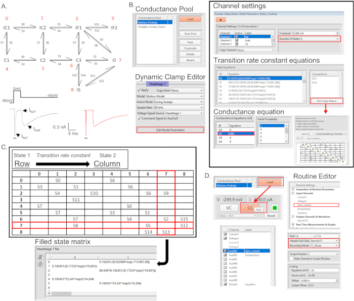
Figure 1: Setting up a Markov model in dynamic clamp software. (A) A Markov state transition diagram is shown for a model that reproduces Nav conductance properties measured in mouse cerebellar Purkinje neurons30. This model includes nine kinetic states. Of these, 8 are non-conducting states: three closed (C), two inactivated-closed (IC), two fast-inactivated (IF), and one slow-inactivated (IS). The model includes one open (O) kinetic state, which is conducting. Between adjacent kinetic states, connections/state occupancy transitioning over time is defined by transition rate constants, shown as S0-S15. Note that each kinetic state is also assigned a numerical value (red), which allows users to define the Markov model and its kinetic state topology in a gating state matrix (shown in panel C, described below). (B) Panels/graphical interfaces that users work with in the SutterPatch Dynamic Clamp Editor are presented. Note, the arrangement of these Dynamic Clamp Editor panels is not consistent with the arrangement as it appears within the dynamic clamp software. Additionally, not all panels associated with the Dynamic Clamp Editor are shown. (C) (upper panel) An example of a gating state matrix is shown with variables entered that correspond to the topology of the state transition diagram shown in panel A. Red boxes on the gating state matrix highlight row and column 7, which correspond to the model's open (O) kinetic state. Within column 7, all rate constants that define transitions into the open (O) kinetic state are listed, and within row 7, all rate constants that define transitions that exit the open (O) kinetic state are listed. With this organization, the gating state matrix describes the number of kinetic states, the rate constant variables, and the topology (interconnections between kinetic states) of the model. Shown in (D) are the SutterPatch panels/user interfaces associated with loading dynamic clamp conductance models, along with the interfaces involved in creating current clamp routines. User interactions with these models are described in Protocol steps 2.17-2.20. Please click here to view a larger version of this figure.

Figure 2: Tsc1mut/mut Purkinje neurons have attenuated membrane excitability compared to wild-type controls. (A) Whole-cell current-clamp recordings from wild type (upper, black) and Tsc1mut/mut (lower, blue) Purkinje neurons reveal attenuated firing in the Tsc1 mutant cell. (B) Reduced firing frequencies in Tsc1mut/mut Purkinje neurons, compared to wild type controls, is consistent across cells. The mean (±± SEM) spontaneous firing frequency of Tsc1mut/mutPurkinje neurons is significantly (P < 0.0001) lower compared to wild type cells (Welch's unpaired t-test; control N = 13, n = 32; Tsc1mut/mut N = 6, n = 21). (C) Voltage-clamp measurements of Nav currents in adult Purkinje neurons reveal that the mean (±± SEM) fast-transient Nav current (INaT) peak is significantly reduced in Tsc1mut/mut cells, compared to wild-type controls. (P = 0.007, RM two-way ANOVA; wild type control: N = 6, n = 22, black; Tsc1mut/mut: N = 6, n = 16, blue squares). Example INaT records, evoked by a -35 mV depolarizing step, are shown as an inset panel to the right of panel C. Data previously published in Brown et al.8. Please click here to view a larger version of this figure.

Figure 3: Using dynamic clamp to determine the effects of an ionic conductance on Purkinje neuron excitability. Dynamic clamp involves sampling membrane voltage (via a recording electrode) and computing, based on the sampled voltage, the current output of a model conductance. The computed current is then applied to a biological cell using a current-injecting electrode. Panel (A) depicts this experimental arrangement. If voltage sampling is performed at a sufficient frequency, and there is minimal delay (latency) between voltage sampling and applying the computed current, this technique can be used to assess how adding or subtracting a modeled conductance affects neuronal firing and membrane excitability. (B) In representative experiments, dynamic clamp recordings were acquired using SutterPatch software and the dPatch amplifier system. dPatch is a patch-clamp amplifier that has external signal processors and a fully integrated digitizer, which makes it well-suited for dynamic clamp recordings (see Discussion). (C) Representative current clamp records of spontaneous Purkinje neuron firing, before and after using dynamic clamp to add or subtract 400 nS of the modeled Nav conductance (presented in Figure 1A). In C1 (left), records are from a Tsc1mut/mut Purkinje neuron with attenuated firing. The addition of 400 nS Nav conductance results in a clear increase in this cell's firing frequency. Alternatively, in C2, records are from a wild-type Purkinje neuron. In this experiment, the modeled Nav conductance is applied with a reversed polarity (-400 nS), resulting in Nav conductance subtraction, and a clear reduction in repetitive firing frequency. Dynamic clamp current injection records, shown in grey, are presented below the action potential firing (voltage) records, shown in black. (D) Results from these dynamic clamp experiments, presented as the changes in spontaneous firing frequency after adding Nav conductance to Tsc1mut/mut Purkinje neurons (D1, n = 3) or subtracting Nav conductance from wild type Purkinje neurons (D2, n = 3), reveals consistent and significant effects of adding or subtracting this conductance across Tsc1mut/mut (P = 0.029) and wild type (P = 0.031) cells, respectively (paired Student's t-test). Please click here to view a larger version of this figure.
Discussion
Cerebellar circuits function in proprioception and motor control37,38 but are also critical for complex behaviors such as social interactions and emotional processing39,40,41. Pathology in cerebellar structure and function is often linked to ASD42,43,44,45,46. The simple architecture of cerebellar circuits47 and the cerebellum's clear role in ASD pathology make it an attractive brain region to investigate the molecular and cellular drivers of ASD behavioral deficits, as well as potential therapeutics. Dynamic clamp electrophysiology offers an important tool for these investigations, enabling investigators to directly test the causal relationships between ASD-related changes in ion channel properties/ionic conductances and the firing of cerebellar neurons. While dynamic clamp methods are particularly suitable for investigations of ASD-related changes in neuronal excitability, this technique is relevant for investigating a range of pathological mechanisms that affect cells with excitable membranes. Additionally, dynamic clamp remains an excellent tool for dissecting the complex processes by which neurons and muscle cells regulate and maintain appropriate action potential firing.
The accurate execution of dynamic clamp experiments requires careful control of technical parameters. Specifically, experimenters should know and understand the consequences of the potential variability in the delay between voltage-sampling and current injection, often referred to as jitter29, as well as electrode passive properties, space-clamp limitations, and the physiological fidelity of the experimental preparation under investigation. Bettencourt et al. (2008)48 and Butera et al. (2001)29 previously showed that achieving high sampling rates of at least 50 kHz is critical for accurately capturing fast ionic conductances, with feedback latencies ideally maintained below 25% (≤ 5 µs) of the sampling interval. Nominal sampling rates reported by commercial systems, particularly Windows-based platforms, can be misleading; hence, independent performance verification is often necessary, which is discussed in more detail by Milescu et al. (2008)25 and Clausen et al. (2012)49. Space-clamp constraints must also be considered, particularly when working with intact neurons that have complex morphologies and non-isopotential membrane properties. For instance, attempting to apply (or subtract) a conductance with an electrode that is distal to the integrating site, such as the AIS, will result in an inaccurate portrayal of the effects of the applied conductance. Poor (high) electrode resistance, inadequate capacitance compensation, and/or failing to correct junction potential error may also cause a misrepresentation of voltage measurements (input signal), and consequently, incorrect application of modeled ionic conductances50,51.
Thousands of Markov and HH models are freely available to researchers in online databases such as ModelDB52 and Channelpedia53, supported by the Human Brain Project and The Laboratory of Neural Microcircuitry, respectively. These databases include models for synaptic conductances, ion channel conductances, and conductance-based neuron models, which are primarily written in NEURON, MATLAB, or Python. Database files typically provide the necessary model equations as well as any miscellaneous information about the cell type(s) and experiments that informed the model.
Both Markov and HH conductance models contain conducting (simulating channels-open/activated) and non-conducting (simulated channels-closed) gating states/variables. However, these model types differ in the way in which the conductance value is calculated at each sampled voltage, with Markov models requiring more computational power but providing more detail in the gating properties of simulated channels. For instance, in HH models, the conducting and non-conducting states are independent variables, each determined by the voltage-input and gating kinetics of the respective state54,55. In contrast with Markov models, HH models do not simulate or constrain the transitions between gating states, such as the transiting of simulated channels from the activated/open kinetic state directly into the fast-inactivated kinetic state in a voltage-gated sodium conductance model25. This makes HH models less computationally complex54,55 and enables investigators to add multiple fast-conductance HH models simultaneously, while maintaining high sampling and update rates.
Markov kinetic state models are composed of discrete kinetic states, which may be conducting or non-conducting, and these states are interconnected in a fixed topology. In Markov model simulations, conductance is calculated at each sampled voltage by the proportion of simulated channels occupying the conducting kinetic state(s). The proportion of simulated channels occupying each kinetic state (over time) is determined by rate constants, which are parameters that govern the rate at which state occupancy transitions from one kinetic state to another. Rate constants have units of inverse seconds (s-1), representing a transition probability per unit of time. Depending on the model, rate constant values may depend on dynamic factors such as voltage or temperature.
In Markov models, ordinary differential equations are used to describe the time-dependent occupancy of each kinetic state. These equations govern how the probability of being in each state evolves over time, based on the transition rate constants. This is represented by a rate matrix Q:  56. As discussed above, transition rate constants (r), which determine the movement between states, may be influenced by the input voltage (V) and parameters α and β, which reflect the kinetics of the conductance across voltages. These equations can be described as:
  , and can be represented visually in the form of graphs that include connections (transition rate constants) into and out of each kinetic state of the model56,57,58. A helpful discussion on the development of Markov models and their topology can be found in Schoening and Silva (2024)56.
Since the inception of dynamic clamp in its current form, in which non-linear ionic conductances are modeled and applied (via current-injecting electrode) to living cells in real-time19,59, the methods and resources for this technique have evolved, and are increasingly accessible and cost-effective due to innovations such as microcontroller-based, low-cost systems60 and free, open-source software23,25,26. Commercial systems, such as Sutter Instrument's dPatch or Cytocybernetics's Cybercyte, further facilitate rapid implementation of dynamic clamp experiments through integrated hardware and software solutions27,61.
The versatility of dynamic clamp enables diverse applications, including the creation of virtual chemical and electrical synapses, embedding real neurons within artificial networks (or vice-versa), and adding virtual ion channels62. Importantly, the voltage-dependence, kinetic properties, and amplitudes of an applied conductance can be rapidly adjusted, allowing investigators to directly test how scaling one or more parameters affects action potential firing and membrane excitability31. Today's systems offer high sampling rates, enabling the accurate application of fast-transient conductances and can be easily integrated with conventional electrophysiological equipment60,63, solidifying dynamic clamp as an ideal method for advancing our understanding of neuronal function and dysfunction.
Disclosures
The authors declare that they have no conflicts of interest.
Acknowledgements
We would like to thank Telly Galiatsatos and Josh Stanford of Sutter Instrument for their assistance in technical inquiries. We also acknowledge and thank Jan Dolzer for help in initiating dPatch dynamic clamp studies.
Materials
| Name | Company | Catalog Number | Comments |
|---|---|---|---|
| CaCl2 | Fisher Chemical | C79-500 | Reagent |
| Capillary glass tubing boroscilicate standard wall OD 1.5 mm ID 0.86 mm length 10 cm | Warner Instruments | 64-0793 | Equipment |
| CleanBench | TMC | 63-9090E | Equipment |
| Compresstome VF-500-Z vibratome | Prescisionary Instruments | https://precisionary.com/product-category/compresstome-parts/parts-by-model/vf-500-0z/ | Equipment |
| Dell OptiPlex 7080 | Dell | https://www.dell.com/en-us/shop/desktop-computers/optiplex-7080-tower-and-small-form-factor/spd/optiplex-7080-desktop/s005o7080sffus | Equipment |
| Dextrose | Fisher Chemical | D16-500 | Reagent |
| dPatch amplifier system | Sutter Instrument | FG-DPATCH | Equipment |
| EGTA | EMD Millipore | 324626-25GM | Reagent |
| HEPES | Fisher Chemical | 7365-45-9 | Reagent |
| In-line heater | Warner Instruments | 64-0102 | Equipment |
| KCl | Fisher Chemical | P330-500 | Reagent |
| Ketamine | Dechra Veterinary Products | 193.40620.3 | Reagent |
| K-gluconate | TCI Chemicals | G0040 | Reagent |
| LinLab software | Scientifica | https://www.scientifica.uk.com/products/scientifica-linlab-2 | Equipment |
| LSE 6L Water Bath | Corning | 6783 | Equipment |
| Mg-ATP | Sigma-Aldrich | 74804-12-9 | Reagent |
| MgCl2 | Fisher Chemical | 012288.A9 | Reagent |
| Model P-1000 Pipette puller | Sutter Instrument | FG-P1000 | Equipment |
| NaCl | Fisher Chemical | S271-500 | Reagent |
| Na-GTP | MP Biomedicals | 56001-37-7 | Reagent |
| NaH2PO4 | J.T. Baker | 02-004-220 | Reagent |
| NaHCO3 | Fisher Chemical | S233-500 | Reagent |
| Ocular software | Digital Optics Limited | https://www.scientifica.uk.com/products/qimaging-ocular-software | Equipment |
| Razor blade | Personna | 60-0139-CTN | Equipment |
| Slice harp | Warner Instruments | 64-0255 | Equipment |
| SliceScope Pro 3000 | Scientifica | https://www.scientifica.uk.com/products/slicescope-pro-3000 | Equipment |
| Superglue | Loctite | 8040-00-142-9193 | Equipment |
| SutterPatch software | Sutter Instrument | https://www.sutter.com/amplifiers/sutterpatch | Equipment |
| Temperature controller | Warner Instruments | 64-2400 | Equipment |
| Xylazine | MP Biomedicals | 158307 | Reagent |
References
- Zoghbi, H. Y., Bear, M. F. Synaptic dysfunction in neurodevelopmental disorders associated with autism and intellectual disabilities. Cold Spring Harb Perspect Biol. 4 (3), a009886-a009886 (2012).
- Isshiki, M., et al. Enhanced synapse remodelling as a common phenotype in mouse models of autism. Nat Commun. 5 (1), 4742(2014).
- Connor, S. A., et al. Altered cortical dynamics and cognitive function upon haploinsufficiency of the autism-linked excitatory synaptic suppressor MDGA2. Neuron. 91 (5), 1052-1068 (2016).
- Pagani, M., et al. mTOR-related synaptic pathology causes autism spectrum disorder-associated functional hyperconnectivity. Nat Commun. 12 (1), 6084(2021).
- Tang, G., et al. Loss of mTOR-dependent macroautophagy causes autistic-like synaptic pruning deficits. Neuron. 83 (5), 1131-1143 (2014).
- Fatemi, S. H., Eschenlauer, A., Aman, J., Folsom, T. D., Chekouo, T. Quantitative proteomics of dorsolateral prefrontal cortex reveals an early pattern of synaptic dysmaturation in children with idiopathic autism. Cereb Cortex. 34 (13), 161-171 (2024).
- Deneault, E., et al. Complete disruption of autism-susceptibility genes by gene editing predominantly reduces functional connectivity of isogenic human neurons. Stem Cell Rep. 11 (5), 1211-1225 (2018).
- Brown, S. P., Jena, A. K., Osko, J. J., Ransdell, J. L. Tsc1 deletion in Purkinje neurons disrupts the axon initial segment, impairing excitability and cerebellar function. Neurobiol Dis. 207, 106856(2025).
- Tsai, P. T., et al. Autistic-like behaviour and cerebellar dysfunction in Purkinje cell Tsc1 mutant mice. Nature. 488, 647-651 (2012).
- Sundberg, M., et al. Purkinje cells derived from TSC patients display hypoexcitability and synaptic deficits associated with reduced FMRP levels and reversed by rapamycin. Mol Psychiatry. 23, 2167-2183 (2018).
- Brumback, A., Sohal, V. Intrinsic excitability defects in specific subtypes of medial prefrontal cortex pyramidal neurons in a mouse model of autism. Neurology. 82 (10), I4-1.010(2014).
- Mitchell, D. E., Miranda-Rottmann, S., Blanchard, M., Araya, R. Altered integration of excitatory inputs onto the basal dendrites of layer 5 pyramidal neurons in a mouse model of Fragile X syndrome. Proc Natl Acad Sci U S A. 120 (2), e2208963120(2023).
- Sanders, S. J., et al. De novo mutations revealed by whole-exome sequencing are strongly associated with autism. Nature. 485, 237-241 (2012).
- Ben-Shalom, R., Keeshen, C. M., Berrios, K. N., An, J. Y., Sanders, S. J., Bender, K. J. Opposing effects on NaV1.2 function underlie differences between SCN2A variants observed in individuals with autism spectrum disorder or infantile seizures. Biol Psychiatry. 82 (3), 224-232 (2017).
- Spratt, P. W. E., et al. The autism-associated gene Scn2a contributes to dendritic excitability and synaptic function in the prefrontal cortex. Neuron. 103 (4), 673-685.e5 (2019).
- Nelson, A. D., et al. Physical and functional convergence of the autism risk genes Scn2a and Ank2 in neocortical pyramidal cell dendrites. Neuron. 112 (7), 1133-1149.e6 (2024).
- Zhang, J., et al. Severe deficiency of the voltage-gated sodium channel NaV1.2 elevates neuronal excitability in adult mice. Cell Rep. 36 (5), 100858(2021).
- Sharp, A. A., Abbott, L. F., Marder, E. Artificial electrical synapses in oscillatory networks. J Neurophysiol. 67 (6), 1691-1694 (1992).
- Sharp, A. A., O'Neil, M. B., Abbott, L. F., Marder, E. The dynamic clamp: artificial conductances in biological neurons. Trends Neurosci. 16 (10), 389-394 (1993).
- Robinson, H. P. C., Kawai, N. Injection of digitally synthesized synaptic conductance transients to measure the integrative properties of neurons. J Neurosci Methods. 49 (3), 157-165 (1993).
- Prinz, A. A., Abbott, L. F., Marder, E. The dynamic clamp comes of age. Trends Neurosci. 27 (4), 218-224 (2004).
- Muñiz, C., Arganda, S., Rodríguez, F. B., De Polavieja, G. G. Realistic stimulation through advanced dynamic-clamp protocols. Computational Methods in Neural Modeling. Mira, J., Álvarez, J. R. , Springer. Berlin. 95-105 (2005).
- Ortega, F. A., Butera, R. J., Christini, D. J., White, J. A., Dorval, A. D. Dynamic clamp in cardiac and neuronal systems using RTXI. Methods Mol Biol. 1183, 327-354 (2014).
- Milescu, L. S., Tabak, J. Dynamic clamp on a Windows PC. Methods Mol Biol. 2188, 157-177 (2021).
- Milescu, L. S., Yamanishi, T., Ptak, K., Mogri, M. Z., Smith, J. C. Real-time kinetic modeling of voltage-gated ion channels using dynamic clamp. Biophys J. 95 (1), 66-87 (2008).
- Kemenes, I., et al. Dynamic clamp with StdpC software. Nat Protoc. 6 (3), 405-417 (2011).
- Dolzer, J. Patch clamp technology in the twenty-first century. Methods Mol Biol. 2188, 21-49 (2021).
- Crino, P. B., Henske, E. P. New developments in the neurobiology of the tuberous sclerosis complex. Neurology. 53 (7), 1384-1390 (1999).
- Butera, R. J., Wilson, C. G., DelNegro, C. A., Smith, J. C. A methodology for achieving high-speed rates for artificial conductance injection in electrically excitable biological cells. IEEE Trans Biomed Eng. 48 (12), 1460-1470 (2001).
- Ransdell, J. L., Moreno, J. D., Bhagavan, D., Silva, J. R., Nerbonne, J. M. Intrinsic mechanisms in the gating of resurgent Na+ currents. eLife. 11, e70173(2022).
- Brown, S. P., Lawson, R. J., Moreno, J. D., Ransdell, J. L. A reinterpretation of the relationship between persistent and resurgent sodium currents. J Neurosci. 44 (29), e2396232024(2024).
- European Chromosome 16 Tuberous Sclerosis Consortium. Identification and characterization of the tuberous sclerosis gene on chromosome 16. Cell. 75 (7), 1305-1315 (1993).
- Henske, E. P., Jóźwiak, S., Kingswood, J. C., Sampson, J. R., Thiele, E. A. Tuberous sclerosis complex. Nat Rev Dis Primers. 2 (1), 16036(2016).
- Wiznitzer, M. Autism and tuberous sclerosis. J Child Neurol. 19 (9), 675-679 (2004).
- Jeste, S. S., Sahin, M., Bolton, P., Ploubidis, G. B., Humphrey, A. Characterization of autism in young children with tuberous sclerosis complex. J Child Neurol. 23 (5), 520-525 (2008).
- Lawson, R. J., et al. Selective deletion of Tsc1 from mouse cerebellar Purkinje neurons drives sex-specific behavioral impairments linked to autism. Front Behav Neurosci. 18, 1474066(2024).
- Sherrington, C. S. The Integrative Action of the Nervous System. , Yale University Press. New Haven. (1911).
- Russell, J. S. R., Horsley, V. A. H. II Experimental researches into the functions of the cerebellum. Proc R Soc Lond. 55, 57-60 (1894).
- Rudolph, S., et al. Cognitive-affective functions of the cerebellum. J Neurosci. 43 (45), 7554-7564 (2023).
- Schmahmann, J. D. The cerebellum and cognition. Neurosci Lett. 688, 62-75 (2019).
- Beuriat, P. -A., Cristofori, I., Gordon, B., Grafman, J. The shifting role of the cerebellum in executive, emotional and social processing across the lifespan. Behav Brain Funct. 18 (1), 6(2022).
- Stoodley, C. J. Distinct regions of the cerebellum show gray matter decreases in autism, ADHD, and developmental dyslexia. Front Syst Neurosci. 8, 92(2014).
- Bruchhage, M. M. K., Bucci, M. -P., Becker, E. B. E. Cerebellar involvement in autism and ADHD. Handb Clin Neurol. 155, 61-72 (2018).
- Mosconi, M. W., Wang, Z., Schmitt, L. M., Tsai, P., Sweeney, J. A. The role of cerebellar circuitry alterations in the pathophysiology of autism spectrum disorders. Front Neurosci. 9, 296(2015).
- Weber, A. M., Egelhoff, J. C., McKellop, J. M., Franz, D. N. Autism and the cerebellum: evidence from tuberous sclerosis. J Autism Dev Disord. 30 (6), 511-517 (2000).
- Wang, S. S. -H., Kloth, A. D., Badura, A. The cerebellum, sensitive periods, and autism. Neuron. 83 (3), 518-532 (2014).
- Ransdell, J. L., Nerbonne, J. M. Voltage-gated sodium currents in cerebellar Purkinje neurons: functional and molecular diversity. Cell Mol Life Sci. 75 (19), 3495-3505 (2018).
- Bettencourt, J. C., Lillis, K. P., Stupin, L. R., White, J. A. Effects of imperfect dynamic clamp: computational and experimental results. J Neurosci Methods. 169 (2), 282-289 (2008).
- Clausen, C., Valiunas, V., Brink, P. R., Cohen, I. S. MATLAB implementation of a dynamic clamp with bandwidth of >125 kHz capable of generating INa at 37°C. Pflugers Arch. 465 (4), 497-507 (2013).
- Preyer, A. J., Butera, R. J. The effect of residual electrode resistance and sampling delay on transient instability in the dynamic clamp system. Annu Int Conf Proc IEEE Eng Med Biol Soc. 2007, 430-433 (2007).
- Preyer, A. J., Butera, R. J. Causes of transient instabilities in the dynamic clamp. IEEE Trans Neural Syst Rehabil Eng. 17 (2), 190-198 (2009).
- McDougal, R. A., et al. Twenty years of ModelDB and beyond: building essential modeling tools for the future of neuroscience. J Comput Neurosci. 42 (1), 1-10 (2017).
- Ranjan, R., et al. Channelpedia: an integrative and interactive database for ion channels. Front Neuroinform. 5, 36(2011).
- Carbonell-Pascual, B., Godoy, E., Ferrer, A., Romero, L., Ferrero, J. M. Comparison between Hodgkin-Huxley and Markov formulations of cardiac ion channels. J Theor Biol. 399, 92-102 (2016).
- Andreozzi, E., Carannante, I., D'Addio, G., Cesarelli, M., Balbi, P. Phenomenological models of NaV1.5. A side by side, procedural, hands-on comparison between Hodgkin-Huxley and kinetic formalisms. Sci Rep. 9 (1), 17493(2019).
- Schoening, M. E., Silva, J. R. Creating Computational Models of Ion Channel Dynamics. Potassium Channels: Methods and Protocols. , Springer. New York. (2024).
- Mangold, K. E., et al. Identification of structures for ion channel kinetic models. PLoS Comput Biol. 17 (8), e1008932(2021).
- Silva, J. R., Cooper, P., Nichols, C. G. Modeling KATP-dependent excitability in pancreatic islets. Biophys J. 107 (9), 2016-2026 (2014).
- Sharp, A. A., O'Neil, M. B., Abbott, L. F., Marder, E. Dynamic clamp: computer-generated conductances in real neurons. J Neurophysiol. 69 (3), 992-995 (1993).
- Desai, N. S., Gray, R., Johnston, D. A dynamic clamp on every rig. eNeuro. 4 (5), (2017).
- Han, L., et al. Reconciling computer models and stem cell models of human cardiac repolarization: reply. Cardiovasc Res. 106 (1), 6-7 (2015).
- Wilders, R. Dynamic clamp: a powerful tool in cardiac electrophysiology. J Physiol. 576 (2), 349-359 (2006).
- Kullmann, P. H. M., Wheeler, D. W., Beacom, J., Horn, J. P. Implementation of a fast 16-bit dynamic clamp using LabVIEW-RT. J Neurophysiol. 91 (1), 542-554 (2004).
Reprints and Permissions
