Semantic Anchor-Aligned Model for Interpretable Video Anomaly Detection under Cross-Modal Weak Supervision

Summary

This protocol aims to improve weakly supervised video anomaly detection by integrating structured knowledge. Its goal is to enable the classification of specific anomaly types and provide clear, interpretable explanations for detection results, moving beyond simple binary decisions and enhancing transparency.

Abstract

Weakly supervised video anomaly detection is a key technique that relies solely on video-level labels to identify anomalous events. However, traditional multiple instance learning (MIL) methods rely on coarse-grained binary supervision. This approach makes it difficult to distinguish between fine-grained anomaly categories. These methods often focus solely on the most anomalous segments, resulting in detection outcomes that lack interpretability. To overcome these limitations, this study proposes a feature modelling approach that incorporates structured knowledge. By utilizing a dynamic semantic guidance mechanism, weakly supervised video anomaly detection combines external category-level information with learnable prompts to generate semantic signals within the feature space. These signals are aligned with the visual evidence extracted by the base anomaly detection module, producing two complementary outputs: an anomaly score for quantifying the severity of anomalous events, and semantic descriptions aligned with external concepts, which can be used to generate structured and interpretable explanatory texts through predefined templates. Experimental results demonstrate that the proposed method achieves an AUC of 88.03% on the UCF-Crime dataset and 98.23% on the ShanghaiTech dataset, attaining 87.05% accuracy in fine-grained anomaly classification tasks. Moreover, the generated semantic explanations extend weakly supervised detection from a binary classification task to a semantics-driven, interpretable anomaly analysis framework.

Introduction

Video anomaly detection (VAD) plays an essential role in fields such as public safety and intelligent manufacturing, where it offers a scalable solution to the limitations of manual surveillance¹. In particular, weakly supervised video anomaly detection (WS-VAD) has gained prominence due to its reliance on video-level labels, substantially reducing the burden of manual annotation while improving generalizability across diverse scenes. Despite its practical advantages, WS-VAD methods still face significant challenges in precisely identifying the nature of abnormal events². Existing models often detect the presence of anomalies but struggle to determine their exact category or provide meaningful diagnostic information^3,4. For instance, in industrial settings, a model might confuse smoke from overheated bearings with harmless steam emissions or incorrectly believe normal welding sparks as early signs of fire, both leading to costly misjudgments and unnecessary shutdowns. These semantic confusions arise from the inherent limitations of current WS-VAD approaches⁵. Binary video-level labels merely indicate whether an anomaly exists, without offering insight into its cause, location, and severity. Moreover, mainstream multiple instance learning (MIL) frameworks⁶ aggregate clip-level predictions using simple heuristics⁷ that fail to capture the nuanced semantics of different event types. As a result, the learned visual feature space becomes ambiguous, where visually similar but semantically distinct phenomena-such as smoke and steam-are mapped too closely, blurring decision boundaries.

Two main research directions have emerged to address these limitations. One focuses on enhancing the MIL framework through improved temporal modeling^4,5,8 or saliency-guided feature selection³. Although such methods improve anomaly localization, they still fall short in offering semantic clarity and interpretability. The other direction involves aligning vision and language representations by integrating pre-trained multimodal models, such as VadCLIP⁹. While this strategy shows promise, it often fails to fully leverage the semantic richness of language. This leads to weak cross-modal associations and opaque decision-making processes, resulting in two core deficiencies. First, current models cannot consistently distinguish between anomaly categories due to vague feature semantics and insufficient external knowledge. Second, the decision-making process contains a black box, without a transparent explanation for why a particular event is classified as anomalous. Although some methods incorporate textual prompts (e.g., fighting, shooting), these are always simplistic and loosely organized, lacking both semantic depth and contextual understanding.

To address these gaps, a new WS-VAD method is introduced that integrates structured external knowledge with interpretable decision mechanisms, a core objective within the broader field of Explainable Artificial Intelligence (XAI)¹⁰. Instead of using basic category names as prompts, the method constructs rich semantic representations-referred to as semantic concept clouds-using Wikidata¹¹. Unlike existing multimodal methods such as VadCLIP⁹ that rely on static text prompts or simple category labels, these semantic concept clouds encapsulate comprehensive contextual knowledge, including related entities, attributes, and causal relationships extracted from structured knowledge graphs. These concept clouds are encoded into semantic anchors by using the BLIP model¹², which enables the system to access fine-grained event semantics. The key innovation of the semantic anchor mechanism lies in its ability to create dynamic, knowledge-enriched representations that adapt to specific anomaly contexts, whereas previous prompt-based methods use fixed textual descriptions that lack contextual depth and semantic relationships. To further refine the feature space, a saliency-guided alignment mechanism selectively associates these anchors with the most relevant visual evidence. This targeted alignment enhances the discriminative power of the features while improving the semantic clarity of the detection results. More importantly, the proposed method supports transparent interpretation. Once a semantic anchor is aligned with visual evidence, the model generates structured natural language explanations using predefined templates, explicitly addressing both the nature and justification of the anomaly. It is important to note that the implementation of this method relies on specific prerequisites, including the use of pre-extracted I3D visual features, access to an external knowledge base (Wikidata), and a pre-trained BLIP encoder. The framework is therefore most beneficial in applications where it is critical to move beyond simple binary detection to instead classify specific anomaly types and provide interpretable justifications for the results.

The key contributions are as follows. A novel WS-VAD method is developed by combining external knowledge with structured interpretability to improve semantic understanding and decision transparency. A semantic embedding-based prompting method and context-aware alignment mechanism are introduced to overcome the limitations of visual-only MIL models. A generative explanation module is incorporated, using semantic anchors as interpretable units to produce coherent textual rationales. Extensive experiments conducted on the UCF-Crime and ShanghaiTech datasets demonstrate the effectiveness of the proposed method, achieving strong AUC scores (88.03% / 98.23%) and superior fine-grained recognition performance, with clear and interpretable outputs.

Protocol

This study uses only publicly available datasets (UCF-Crime¹³ and ShanghaiTech¹⁴). All videos were obtained from the official releases of the datasets, which anonymize personally identifiable information to the extent provided by the dataset maintainers. No additional data collection or human subject interaction was conducted by the authors; therefore, no new IRB approval was required. Data usage complies with the licenses and terms of use of the respective datasets.

Data preparation and feature extraction

Dataset preparation:The UCF-Crime¹³ (1,610 train/290 test videos) and ShanghaiTech¹⁴ (238 train/199 test videos) datasets were adopted under their standard splits. Videos were preprocessed using FFmpeg to ensure reproducibility, re-encoded to H.264, resampled to 25 fps, and resized to 256 x 256 resolution with the command: ffmpeg -i v.mp4 -vf "fps=25,scale=256:256" -c:v libx264 -crf 23 -preset veryfast pre/.

Feature extraction: RGB features were extracted by an I3D backbone¹⁵ pre-trained on the Kinetics dataset¹⁶. Videos were split into non-overlapping 16-frameclips; each clip was center-cropped to 224 x 224 pixels. The penultimate layer activations were average-pooled to obtain a 1024-D feature per clip. In PyTorch, this corresponds to forwarding tensors of shape [B, 3, T, H, W] through the I3D backbone and applying adaptive_avg_pool3d followed by flattening. The extracted features were saved in .npy files (one per video) together with clip timestamps for exact reproducibility (seed = 123). For each video, features///

Model architecture and methodology

Basic detection: temporal context fusion
Given a video clip sequence represented by a feature matrix Z  R^Tx1024, the Temporal Context Fusion (TCF) module first computed query, key, and value representations through three learned linear projections:

Q = ZW^Q, K = ZW^K, V = ZW^V (1)

where W^Q, W^K, W^V  R^Tx1024xd are trainable parameters (PyTorch: three nn.Linear (1024,d) layers). The intersegment affinity was S = , a Temporal Relationality Embedding (TRE) was incorporated, where each element was computed as R_ij = α exp () + β . The location-aware affinity was = S + R. A global-context map  A = softmax() aggregated V  to obtain wide-area features G = AV. Local features L were computed with a depthwise 1-D convolution (nn.Conv1d) of kernel size 3 over Z. A dynamic gate g = σ(MLP ([G;L]))  mixed the two: U = g G + (1 - g) L . Finally, layer normalization and a residual linear layer were applied to produce Y (Pytorch:LayerNorm+Linear+residual).

Basic detection: causal temporal predictor

The output Y was passed through two causal 1-D convolutions with GELU and dropout (Pytorch:padding='causal' or masked conv) to obtain per-clip anomaly logits. Applying the sigmoid function yielded probability values  [0,1]^T.

Semantic enhancement: prompt learning with external knowledge

Construct semantic anchors : For each anomaly class c, K_c concepts were queried from Wikidata¹¹, and encoded each concept phrase was encoded with BLIP's¹²text encoder to e_i  R⁷⁶⁸. The class anchor was the l₂-normalized mean D_c = norm(Σ_ie_i) . To reduce noise, concepts with cosine similarity to the class name below 0.2 were dropped, and the top-M by TF-IDF score were kept.

Perform context-sensitive separation : Foreground weights α_t = softmax(rs_t) were computed from base detector scores s_t, and background weights bt = softmax(r(1 - s_t)). The weighted features are f_fg = Σ_tαz_t and f_bg = Σ_tbz_t .

Align visual and semantic features

Define the alignment objective: During the alignment step, the objective is to minimize the distance between the foreground visual feature and its corresponding semantic anchor of the anomalous category within the feature space. Create a collection of semantic guides, , comprising C anomalous category semantic guides and one standard normal semantic guide. Determine the likelihood, P(D^k|v), that a visual feature, v, corresponds to the k-th semantic guide, D^k. Calculate this using temperature-scaled cosine similarity followed by Softmax normalization, as shown in Eq. 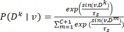(2).

  (2)

Cross-entropy was minimized to push positive pairs together and negatives apart, with being set τ_s as a learnable parameter and initializing it to 10. Accomplish the alignment by optimizing the likelihood of correlating positive sample pairs while reducing the likelihood of correlating negative sample pairs.

Template-based interpretability module

Based on the prompt learning with external knowledge (PLE)-enhanced feature representation, a linear classifier produces per-class logits, which were subsequently normalized into class probabilities by the softmax function; the predicted anomaly type was determined as the category with the highest probability. Meanwhile, a global anomaly score was computed from the detector output. To determine the severity level, this score was compared against three predefined thresholds optimized through grid search on the validation set.

The default thresholds were set to θ_high = 0.8, θ_medium = 0.5, and θ_low = 0.2. Specifically, if the score was greater than θ_high, the severity was labeled as high; if the score falls between θ_medium and θ_high, it was labeled as medium; if between θ_low and θ_medium, it was labeled as low; otherwise, it was marked as none.

During the explanation generation phase, a template corresponding to the predicted type was selected from a predefined template library, Supplementary File 1. This library contains multiple template variants that have been cross-validated by multiple annotators¹⁷ to enhance the diversity of the generated text. If the predicted type exists in the template library, a corresponding template was randomly selected; otherwise, a default template for the Unknown type was used. Finally, a structured explanatory text was generated by integrating the predicted type, global anomaly score, severity description, and the selected template. The system returns the predicted anomaly type, global anomaly score, and the generated explanatory text as the final output. The results are illustrated in Figure 2.

All threshold parameters were optimized using grid search on the validation set, and the quality of the generated explanations was comprehensively evaluated using both human assessment and automated metrics. The results are presented in Table 1.

Model training and evaluation

Training: The model was trained end-to-end with Adam (lr 1 x 10^-4, weight decay 5 x 10^-4), batch size 128, 50 epochs, cosine annealing for lr. Random seeds were set to 123 for Python/Numpy/Pytorch and enabled torch.backends.cudnn.deterministic=True. Checkpoints were saved every 5 epochs to checkpoints//epoch_XX.pt, and the best model was selected by validation AUC. All experiments were conducted on a system with an NVIDIA GeForce RTX 4060 Ti (16GB) GPU running Windows 11, with Python 3.8.20, PyTorch 1.8.0, and CUDA 11.1. The approximate training time per epoch was 30 s for the ShanghaiTech dataset and 3.5 min for the UCF-Crime dataset.

Loss: The overall objective is L = L_MIL+ λ • L_align. The hyperparameter λ was swept across the set {0.01,0.1,0.5,1,5,10} on the validation set, and fixed the best value was fixed for test reporting. See Figure 3 for top-K MIL aggregation and Eq.(3-4) for definitions.

 (3)

 (4)

Evaluation: Frame-level AUC was computed following the standard protocol used by prior WS-VAD works^2,5. For fine-grained type recognition on UCF-Crime, mAP at IoU 0.1-0.5 and AVG mAP were reported, as summarized in Table 2; per-class AUCs are shown in Figure 4 and overall results in Table 3 and Table 4; embedding separability and anomaly-score dynamics are in Figure 4, Figure 5, and Figure 6.

Results

To further validate the utility of semantic anchors, an additional experiment was conducted to compare different prompt templates (see Table 1). The variant using Wikidata-augmented semantic prototypes not only achieved higher AUC values but also led to BLEU-4 score improvements of 16.6 and 14.8 for the generated explanations. These findings indicate a strong link between the semantic richness of prompts and the quality of textual interpretations, confirming that the explanation generation process goes b...

Discussion

The protocol presented here introduces a significant advancement in weakly supervised video anomaly detection by shifting the paradigm from simple binary classification to a semantically grounded, interpretable analysis. The significance of this method lies in its ability to not only identify if an anomaly occurred but also what kind of anomaly it is and why the model reached that conclusion, addressing a major limitation in existing WS-VAD systems^9,29.

Materials

List of materials used in this article

Name	Company	Catalog Number	Comments
BLIP Model	Salesforce Research	ViT-B/16	Used as the text encoder for creating semantic anchors.
GPU	NVIDIA	RTX 4060Ti	Used for training the model
I3D Model	Google DeepMind	Pre-trained on Kinetics	Used as the backbone for video feature extraction.
Numpy	The NumPy Development Team	1.21.2	Used for handling and processing numerical data arrays, such as the video features, before they are fed into the deep learning model.
PyTorch	Facebook AI Research	1.8.0	Used for defining the model architecture, implementing the custom loss functions, and running the back-propagation for optimization.
Python	Python Software Foundation	3.8.20	Used to write all scripts for data processing, model implementation, training, and evaluation
ShanghaiTech Dataset	ShanghaiTech University		Used for training and evaluation in 13 different campus scenes.
UCF-Crime Dataset	University of Central Florida		Used for training and evaluation of 13 anomaly categories.
Wikidata	Wikimedia Foundation		Used as the external knowledge graph for prompt construction.

References

- Abdalla, M., Javed, S., Radi, M. A., Ulhaq, A., Werghi, N. Video anomaly detection in 10 years: A survey and outlook. arXiv. , (2024).
- Caetano, F., Carvalho, P., Mastralexi, C., Cardoso, J. S. Enhancing weakly-supervised video anomaly detection with temporal constraints. IEEE Access. 13, 70882-70894 (2025).
- Dual memory units with uncertainty regulation for weakly supervised video anomaly detection. Zhou, H., Yu, J., Yang, W. Proc AAAI Conf Artificial Intell, 37 (3), 3769-3777 (2023).
- Dynamic local aggregation network with adaptive clusterer for anomaly detection. Yang, Z., Wu, P., Liu, J., Liu, X. Proc Eur Conf Comp Vision, 13664, 404-421 (2022).
- Pu, Y., Wu, X., Yang, L., Wang, S. Learning prompt-enhanced context features for weakly-supervised video anomaly detection. IEEE Trans. Image Process. 33 (8), 4923-4936 (2024).
- Look around for anomalies: Weakly-supervised anomaly detection via context-motion relational learning. Cho, M., et al. Proc Conf Comp Vision Pattern Recognit, , 12137-12146 (2023).
- Tian, Y., et al. Weakly-supervised video anomaly detection with robust temporal feature magnitude learning. Proc Int Conf Comp Vision. , 4955-4966 (2021).
- Scale-aware spatio-temporal relation learning for video anomaly detection. Li, G., Cai, G., Zeng, X., Zhao, R. Proc Eur Conf Comp Vision, , 333-350 (2022).
- Vadclip: Adapting vision-language models for weakly supervised video anomaly detection. Wu, P., et al. Proc Conf Artificial Intell, 38 (6), 6074-6082 (2024).
- Hosain, M. T., Jim, J. R., Mridha, M. F., Kabir, M. M. Explainable AI approaches in deep learning: Advancements, applications, and challenges. Comp Elect Eng. 117, 109246(2024).
- Vrandecic, D., Kroetzsch, M. Wikidata: A free collaborative knowledgebase. Comm ACM. 57 (10), 78-85 (2014).
- Blip: Bootstrapping language-image pre-training for unified vision-language understanding and generation. Li, J., Li, D., Xiong, C., Hoi, S. Proc Int Conf Machine Learning, 162, 12888-12900 (2022).
- Real-world anomaly detection in surveillance videos. Sultani, W., Chen, C., Shah, M. I. Proc Conf Comp Vision Pattern Recognit, , 6479-6488 (2018).
- Future frame prediction for anomaly detection - a new baseline. Liu, W., Luo, W., Lian, D., Gao, S. I. Proc Conf Comp Vision Pattern Recognit, , 6536-6545 (2018).
- Quo vadis, action recognition? A new model and the kinetics dataset. Carreira, J., Zisserman, A. Proc Conf Comp Vision Pattern Recognit, , 6299-6308 (2017).
- Kay, W., et al. The kinetics human action video dataset. arXiv. , (2017).
- Purba, M., et al. Effect of random splitting and cross validation for Indonesian opinion mining using machine learning approach. Int J Adv Comp Sci Appl. 13 (9), 145-151 (2022).
- Wu, P., Liu, X., Liu, J. Weakly supervised audio-visual violence detection. Ieee Transact Multimedia. 25, 1674-1685 (2023).
- Liu, T., Lam, K. M., Bao, B. K. Injecting text clues for improving anomalous event detection from weakly labeled videos. Ieee Transact Image Proc. 33, 5907-5920 (2024).
- Wu, P., Liu, J. Learning causal temporal relation and feature discrimination for anomaly detection. Ieee Transact Image Proc. 30, 3513-3527 (2021).
- Assoc Advancement Artificial, I. Self-training multi-sequence learning with transformer for weakly supervised video anomaly detection. Li, S., Liu, F., Jiao, L. Proc Conf Artificial Intell, 36 (2), 1395-1403 (2022).
- Normality guided multiple instance learning for weakly supervised video anomaly detection. Park, S., et al. Proc Winter Conf Appl Comp Vision, , 2664-2673 (2023).
- Zanella, L., et al. Delving into clip latent space for video anomaly recognition. Comp Vision Image Understanding. 249, 104163(2024).
- Prompt-enhanced multiple instance learning for weakly supervised video anomaly detection. Chen, J., et al. Proc Conf Com Vision Pattern Recognit, , 18319-18329 (2024).
- Distilling aggregated knowledge for weakly-supervised video anomaly detection. Dalvi, J., Dabouei, A., Dhanuka, G., Xu, M. Proc Winter Conf Appl Comp Vision, , 5439-5448 (2025).
- Gods: Generalized one-class discriminative subspaces for anomaly detection. Wang, J., Cherian, A. I. Proc Int Conf Comp Vision, , 8200-8210 (2019).
- Biswas, D., Tesic, J. Mmvad: A vision-language model for cross-domain video anomaly detection with contrastive learning and scale-adaptive frame segmentation. Exp Syst Appl. 285, 127857(2025).
- Lim, J., Lee, J., Kim, H., Park, E. Vicap-ad: Video caption-based weakly supervised video anomaly detection. Machine Vision Applicat. 36 (3), 61(2025).
- Gao, W., Wang, X., Wang, Y., Jing, X. Dual-stream attention-enhanced memory networks for video anomaly detection. Sensors. 25 (17), 5496(2025).
- Duong, H. T., Le, V. T., Hoang, V. T. Deep learning-based anomaly detection in video surveillance: A survey. Sensors. 23 (11), 5024(2023).
Access restricted. Please log in or start a trial to view this content.