A Comparative Approach for Quantitative Cell Counting Studies in Widely Different Mammalian Brains

Summary

Modern neurosciences need to explore differences among many species, including laboratory rodents and humans. Yet technical difficulties arise when large-brained mammals are involved. This approach addresses interspecies variation of neuronal populations in widely different mammals, yielding comparable results to be mapped for revealing evolutionary patterns.

Abstract

Most neurobiological studies are conducted on laboratory rodents. Despite many similarities across mammalian brains, important differences also exist, which can be misleading in translation. Marked interspecies differences have been found in brain plasticity, particularly neurogenesis. Different neurogenic processes can be prevalent because of evolutionary tradeoffs, displaying variation across brain structures and mammals and shifting the potential for plasticity in divergent species, such as mice and humans. Comparing widely different species raises multiple issues: comparative studies encounter technical difficulties when large-sized brains are involved; the use of heterogeneous experimental approaches by different laboratories can limit the comparison of results; heterogeneity may be related to different time courses of neurodevelopmental processes across mammals, thus adding variables to the comparison.

To tackle these limitations, an approach to study the interspecies variation of a population of layer II cortical immature neurons in mammals widely differing for brain size, gyrencephaly, socioecological niche, and age was established. Despite some variables that cannot be fully standardized, a method that combines reduced heterogeneity in collecting brains and the establishment of common anatomical structures as reference points for performing the cell counting on corresponding brain levels is proposed. Data obtained (e.g., cell densities) can be mapped onto phylogenetic trees to reveal evolutionary patterns and analyzed for covariance with neuroanatomical features (e.g., brain size, cortical surface area). This approach has demonstrated remarkable variation in the number of cortical immature neurons between phylogenetic groups and uncovered covariation with brain size. The method can also be used to quantify differences through different developmental stages in the same species and can be extended to other diverse mammals and biological processes to map comparable results that allow for more accurate quantification of different cell populations in adult brains to support plasticity.

Introduction

Neuroscience research largely uses inbred mice and rats to translate results to humans. Despite many molecular, cellular, and even anatomical similarities, important interspecies differences also exist, which can be misleading for the interpretation of preclinical data^1,2. Though comparative studies are needed, they are hindered by technical and practical difficulties when large-sized brains are involved (e.g., from an average of 0.5 g in mice to 1300 g in humans; Figure 1A). Moreover, heterogeneous experimental approaches by different laboratories can limit the comparison of results, especially quantitative analyses, sometimes generating controversies. This is the case of brain structural plasticity, with special reference to neurogenic processes^3,4,5, a topic that is of interest in understanding developmental neuroplasticity and brain repair^6,7.

Recent discoveries in the field of brain plasticity strongly suggest that substantial differences emerged during evolution in the occurrence, rate, and anatomical location of different types of neurogenic processes⁸. An example is given by the evident decrease of stem cell-driven neurogenesis occurring in adult large-brained mammals compared with laboratory rodents^5,9,10, likely linked to different expansion of brain regions and functions as an adaptation to ecological pressures^7,8, as well as to different neurodevelopmental time courses^11,12. The rate of neurogenesis appears to differ remarkably between mice and humans, thus raising the issue of translation¹³.

On the other hand, a novel kind of "neurogenesis without division" represented by neurons blocked in arrested maturation (so-called immature or dormant neurons^{14,15,16,17,18,19}) has been hypothesized to increase from small-brained to large-brained species^20,21. Interestingly, the stem cell-independent population of immature neurons is hosted in the cerebral cortex (a site of high-order cognition in gyrencephalic species^22,23) and far from the canonical neurogenic sites, which are mostly linked to olfaction and spatial navigation, which retain great importance in lissencephalic species^7,8. These differences across brain structures and mammal species go beyond sheer comparative interest since they can be relevant in translation by shifting the potential for plasticity in mice and humans. For these reasons, it is crucial to assess in a "comparable way" to what extent the differences represent a phylogenetic variation across widely different mammals, with special reference to laboratory rodents and primates.

An approach recently established to study the interspecies variation of a population of layer II cortical immature neurons (cINs) in mammals widely differing in brain size, gyrencephaly, and socioecological niche^22,24,25is described. This method is based on three principles: i) to consider several (diverse) mammalian species to be processed in parallel using the same procedures; ii) to minimize variables that cannot be fully standardized in widely different brains (fixation procedure, postmortem interval, age) and to address the species-specificity of antibodies for immunocytochemistry by using widely shared features of the cell population under study as internal positive controls; and iii) to establish corresponding anatomical structures as reference points for performing the cell counting on correspondent brain levels of different species (Figure 1B and Figure 2). Data obtained (e.g., cell densities) by counting cells identified with the well-established marker doublecortin (DCX^15,17,26) can be mapped onto phylogenetic trees to reveal evolutionary patterns and analyzed for covariance with different parameters, such as brain size, gyrencephaly, and cortical surface area.

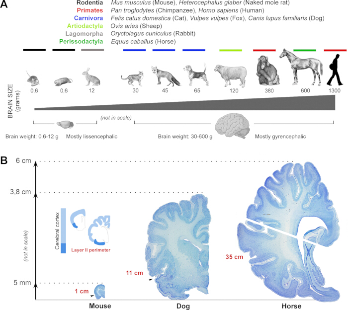
Figure 1: Processing of widely different mammalian brains for assessing the distribution and amount of cINs in the cortical mantle. (A) Mammals belonging to different species and orders are characterized by widely different brain sizes and degrees of gyrencephaly and cortical expansion. Brain icons reproduced with BioRender license. (B) Representative Toluidine blue-stained coronal sections cut from brains of widely different sizes and cortical mantle extension. Histologically stained serial sections (cryostat cut, coronal, 40 µm thick) are used to identify the main neuroanatomical structures in each animal species (see Figure 3); note the remarkable differences in brain size and cortical perimeter. The animal icons in panel A have been reproduced with permission from La Rosa et al.²². Please click here to view a larger version of this figure.

Finally, since all plastic processes generally undergo progressive reduction with increasing age^27,28, one further issue in comparative neuroplasticity is to assess the different time courses of such a reduction, which may be related to different time courses of neurodevelopmental processes across mammals^12,29,30. As a matter of fact, the existence of fast-maturing (mouse) versus slow-maturing species (primates) is another reason why the most common model system, the laboratory mouse, is limited in resolving challenges in biomedical sciences. The method described here can also be useful to consider cell populations at different ages across the lifespan of each species and then compare the resulting trends among species. Phylogenetic variation in the cIN density, as well as differences in their persistence through ages, were found between small-brained and large-brained mammals^22,28.

Protocol

All animal procedures complied with the relevant national and institutional regulations. Mouse tissues were obtained from the Neuroscience Institute Cavalieri Ottolenghi (NICO), Orbassano, Italy, under authorization from the Italian Ministry of Health (RRID: MGI:3696370), courtesy of Serena Bovetti and Charles River Laboratories. Naked mole rat tissues were collected at Queen Mary University of London (UK) immediately after euthanasia according to Schedule 1 of the Animals (Scientific Procedures) Act 1986. Rabbit experiments followed the European Communities Council Directive 86/609/EU and Italian law (DL.vo 116/92), with approval from the Italian Ministry of Health (authorization 66/99-A). Sheep and horse brains were obtained postmortem from a commercial slaughterhouse under Directive 86/609/EEC and continuous veterinary supervision. Dog brains were supplied postmortem by MarshallBio Laboratories (Lyon, France) with the required authorizations; cat brains were collected postmortem at the University of Padova during routine diagnostic necropsies with owner consent. All procedures followed EU and Italian legislation. Chimpanzee samples were handled according to Council for International Organizations of Medical Sciences (CIOMS) international guiding principles and under National Institutes of Health-Office of Laboratory Animal Welfare (NIH-OLAW) permit A5761-01 (for details in each animal species and experiment see Supplementary Table 1 and Ref.^22,25).

1. Collecting brains

1. Collect brains directly or from other Institutions and tissue banks, but consider only the entire hemispheres. Set up with the institutions the best procedure to extract brains from the animal species, considering to lower the damage to the hemisphere and to ensure the minimum postmortem interval (PMI, see NOTE below) and fast immersion in fixative solution after extraction.
   NOTE: Depending on the sensitivity of the antibody of interest, be aware of the PMI. Given the high sensitivity of doublecortin (DCX) to degradation, collect samples with a PMI range of 0-1 h (aside from the chimpanzee, having up to 14 h PMI, which, however, did not cause any alteration in the quality of staining, Supplementary Table 1).
2. Given the high variability of the animal's lifespan, pre-determine the age groups that will be collected among the different mammals considered for the study, to obtain comparable data.
   1. For this study design and to set comparable age groups, analyze information from two databases on animal history and diversity: AnAge, a curated database of ageing and life history in animals, and Animal Diversity Web, an online database of animal natural history, distribution, classification, and conservation biology.
   2. Divide the animal lifespan into four stages (one prepuberal and three postpuberal, namely, "adult"), starting from the classification of the American Veterinary Medical Association (AVMA) for life stages in dogs³¹, in which the lifespan was divided into six stages: puppy, junior, adult, mature, senior, and geriatric.
   3. By compacting the senior and geriatric, and the adult and mature stages, apply this terminology: prepuberal, young-adult, middle age, and senior/aged²².

2. Brain tissue fixation and processing

NOTE: Fixation procedures can be different depending on brain size and ethical concerns regarding some animal species (most large-brained primates or horses cannot be perfused and must be fixed by immersion in the fixative solution after extraction).

1. Keep brains completely immersed in fixative solution (4% paraformaldehyde or 10% formalin recommended).
   NOTE The time of fixation varies depending on brain size (e.g., 3 weeks for canine brain; 3 months for equine brain, Supplementary Table 1). Avoid low/excessive time in the fixative solution to maintain the integrity of the antigen of interest.
2. Cut the preferred brain hemisphere into equal slices (1-1.5 cm thick) using a ruler (to perform a straight cut) and a stab knife.
3. Immerse brain slices in phosphate buffer (PB) 0.1 M (28.49 g sodium phosphate dibasic and 7.8 g sodium phosphate monobasic dissolved in distilled water, pH 7.4) and keep them under gentle agitation on a shaker for 24 h. If needed (see NOTE below), discard the solution and replace it with a fresh solution of PB 0.1 M, pH 7.4 on the next day.
   NOTE: The volume and number of washings in PB 0.1 M vary depending on brain size (e.g., 30 min for mouse brain, 3 days for horse brain). Make sure that brains are entirely immersed in PB 0.1 M and that formalin, blood and tissue waste are no longer present to stop washing.
4. Cryoprotect the slices by immersing them in sucrose solutions of gradually increasing concentration (10%, 20%, up to 30%) in PB 0.1 M, pH 7.4, and keep them under gentle agitation on a shaker.
   NOTE: The volume of sucrose solutions varies depending on brain size. Make sure that brains are entirely immersed in sucrose solutions and that they sink completely before moving them into increased sucrose concentration.

3. Whole hemisphere cryostat cutting

1. Remove meninges from the brain slices using curved tweezers to avoid issues during cutting.
2. Put the slices into embedding molds filled with optimal cutting temperature (OCT) compound. If the slice does not fill the embedding mold, cut a square piece of Parafilm slightly larger than the brain slice and add OCT medium to the center of the piece, then place the slice on top of the OCT.
3. Freeze the slice by immersion in 300 mL of liquid nitrogen-chilled isopentane at -50 °C until the OCT medium turns entirely white. Brain slices can be kept at -80 °C for long-term storage until sectioning.
4. Before sectioning, keep the brain slice at -20 °C for at least 5 h to allow the tissue to slowly and homogeneously reach the same temperature as the cryostat.
5. Cut the slice into 40 µm thick serial coronal sections using a cryostat, maintaining an inside chamber temperature range of -20 °C to -25 °C.
6. Collect free-floating sections in 12-well plates and store them in cryoprotectant solution (150 mL of glycerol, 150 mL of ethylene glycol, 150 mL of distilled water, and 50 mL of F buffer [1.682 g of sodium phosphate monobasic dihydrate and 0.385 g of sodium hydroxide dissolved in distilled water, pH 7.4]) (1 mL/well, or more to completely cover the sections in the case of large brains) at -20 °C until staining.
   NOTE: Whole hemisphere slices vary depending on brain size. Larger brains (e.g., chimpanzees, horses) need to be divided into two equal blocks (dorsal and ventral) to be processed in the cryostat. In this case, free-floating sections can be collected in two 6-well plates. An alternative is to section hemispheres from large-brained species with a sliding microtome, which allows for blocks of larger size.

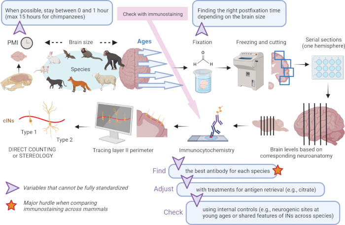
Figure 2: Processing widely different brains following the same procedure and dealing with variables that cannot be standardized. In the method described above, all procedures that can be standardized are performed in the same way (general fixation, cutting serial coronal sections of the same thickness in the whole hemisphere, general immunocytochemical procedures, cell counting). Figure created with BioRender (https://app.biorender.com/). Please click here to view a larger version of this figure.

4. Histological staining

1. Pick serial coronal sections (1 section out of 12). To obtain this spacing, pick all the sections of one well from the 12-well plate. Use them to obtain a full representation of the whole hemisphere and as a reference to pick coronal sections at different comparable brain levels among the different species studied (see section 5). Mount them on 1% gelatinized slides. Let them dry for a few hours.
2. Prepare the following solutions (150 mL/solution): ethanol 50%, 70%, 96%, 100%, Xylol, and Toluidine Blue.
3. Staining protocol: Place the slides in increasing concentrations of ethanol (50%-100%), 1 min each at 50%-70%, 2 min each at 96%-100%, and then transfer to xylol solution for 1 min.
4. Place the slides in the reverse order: xylol solution for 1 min and then decreasing concentrations of ethanol solutions (100%-50%), 2 min each at 100%-96%, 1 min each at 70%-50%.
5. Place the slides in 150 mL of distilled H₂O (2 min).
6. Place the slides in the Toluidine Blue stain solution (5-10 min). After this step, stained sections appear dark blue.
   NOTE: The time sections are kept in the solutions for histological staining can differ depending on the species. Test brain sections of the species of interest to set the optimal staining protocol.
7. Rinse the slides in 150 mL of distilled H₂O for 1 min.
8. Proceed with the differentiation step by placing the slides in increasing concentrations of ethanol (70%-100%) for 1 min at 70%, 2 min each at 96%-100%, and then transfer to xylol solution for 1 min 30 s. During these steps, sections will shift from a dark blue to a sky-blue color.
9. Ensure the sections are still wet from the last xylol step before cover slipping using mounting medium (if they dry, rinse them in xylol solution for 5 s). Then let the slides dry for a few days.

5. Brain levels selection and immunohistochemical staining

1. Using the histologically stained sections obtained in section 4 as reference, identify brain levels depending on specific neuroanatomical features: Level 1 (L1) - from anterior opening of the lateral ventricle to L2; Level 2 (L2) - from anterior starting of internal capsule to L3; Level 3 (L3) - from anterior starting of the amygdala to L4; Level 4 (L4) - from posterior closing of the lateral ventricle to an extension equivalent to that of L2 (same number of 40 µm thick serial sections; Figure 3).
   NOTE: The neuroanatomical references listed above have the purpose of allowing the comparison of the cerebral cortices belonging to brains of widely different size and gyrencephaly. Depending on the brain region of interest, the anatomical features used as reference can change.
2. Pick three equally spaced coronal sections from each brain level.
   NOTE: The volume of each buffer used in the next steps varies depending on brain size (e.g., 0.5 mL/well for mouse sections, 1.5 mL/well for horse sections). Make sure that the free-floating sections are entirely covered by each buffer.
3. Wash sections three times in PBS 0.01 M, pH 7.4, for 5 min each.
4. Incubate sections in endogenous peroxidase blocking solution (0.6% H₂O₂, 1% Triton X-100 in 0.01 M PBS, pH 7.4; 20 min) or perform antigen retrieval using citric acid (10 mM citric acid in distilled water supplemented with 0.05% Tween 20, pH 6.0), 5 min at 90 °C.
   NOTE: Depending on the fixation procedure/time and the antigen of interest, an antigen retrieval may be required to obtain optimal staining (buffer, temperature, pH, and incubation time used may vary depending on the antigen of interest).
5. Wash sections again in PBS 0.01 M, pH 7.4 (3 x 5 min washes).
6. Incubate sections in blocking solution (1-5% bovine serum albumin (BSA), normal serum, 1-1.5% Triton X-100 in 0.01 M PBS, pH 7.4; 90 min at RT).
7. Incubate sections with primary antibody solution (1-5% BSA, 2-3% normal serum, 1-1.5% Triton X-100, primary antibody in 0.01 M PBS, pH 7.4; 48 h at 4 °C under gentle stirring).
   NOTE: Antibodies against the antigen of interest may give different results in terms of quality of staining when used in different brain regions and in different species²⁶. A comparison between a set of antibodies from different manufacturers is needed to choose the optimal tool to be used in the different species considered for the study (to reduce variability among samples).
8. Repeat the washing step described in step 5.3.
9. Incubate sections with secondary biotinylated antibody solution (1-5% BSA, 2-3% normal serum, 1-1.5% Triton X-100, secondary biotinylated antibody in 0.01 M PBS, pH 7.4; 2 h at RT).
   NOTE The avidin-biotin peroxidase complex method is used for the cell counting on Neurolucida (see section 6), since it gives a dense, long-lasting precipitate, thus allowing for focusing through the section thickness while counting. Immunofluorescence and confocal analysis can also be used to perform double/triple immunostaining to further characterize the cells (for protocols see Ref.^22,25,32).
10. Prepare avidin-biotin-peroxidase complex using the available kit.
    NOTE: Prepare avidin-biotin peroxidase complex solution in Tris-HCl 0.05 M, pH 7.5 (which provides a stable pH for complex formation) at least 1 h before use, to allow complex formation.
11. Wash sections twice in PBS 0.01 M, pH 7.4 (2 x 5 min washes), and once in Tris-HCl 0.05 M, pH 7.5 (5 min).
    NOTE: Since the avidin-biotin-peroxidase complex is in solution with Tris-HCl 0.05M, rinsing with Tris-HCl 0.05 M allows habituation of the tissue to the solution.
12. Incubate sections in avidin-biotin-peroxidase complex (1 h at RT).
13. Wash sections in Tris-HCl 0.05 M, pH 7.5 (3 x 5 min washes).
14. Under a fume hood, incubate sections in 3,3'-diaminobenzidine (DAB) staining solution (H₂O₂, DAB in Tris-HCl 0.05 M, pH 7.5) until the optimal staining is obtained. During this step, the sections shift from a transparent to a brown/burgundy red color.
    NOTE: The time to obtain the optimal staining varies depending on the species analyzed (e.g., for DCX, 2-5 min for mouse sections, 20-30 min for horse sections). Check sections staining every 2 min to avoid overstaining.
15. Wash sections in PBS 0.01 M, pH 7.4 (3 x 5 min washes).
16. Mount sections on a slide, once dry, cover with a coverslip using mounting medium, and let the slides dry for a few days.

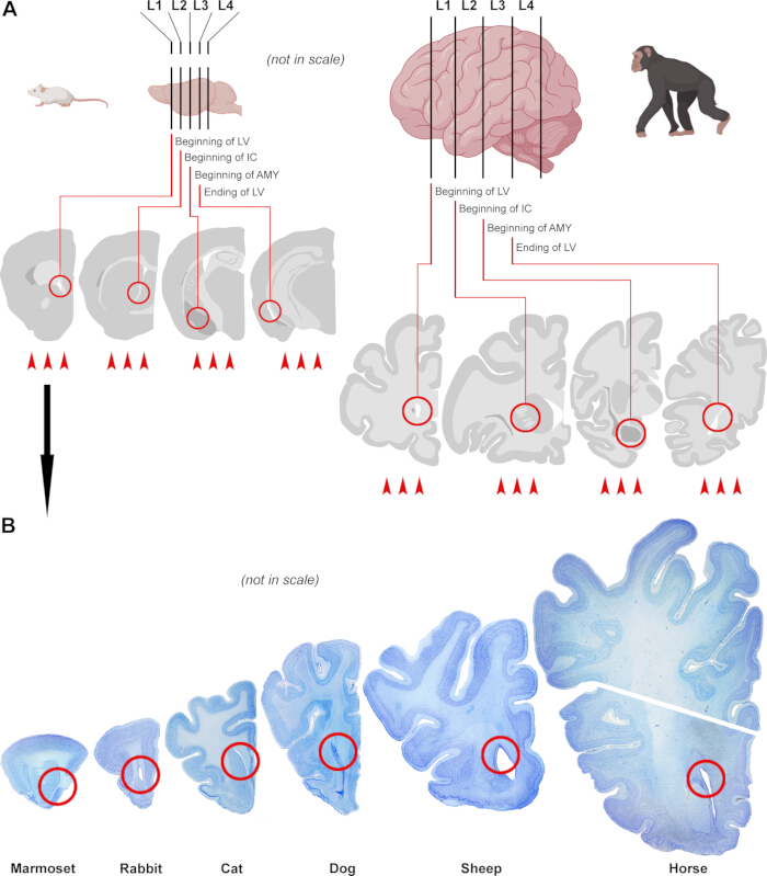
Figure 3: Establishing neuroanatomical brain levels for the study of DCX+ immature neuron distribution and amount in the cerebral cortex. Four corresponding neuroanatomical structures (anterior starting of the lateral ventricle [level 1, L1]; anterior starting of the internal capsule [L2]; anterior starting of the amygdala [L3]); posterior closing of the lateral ventricle [L4]; indicated by red circles) were considered to establish four corresponding anterior-to-posterior "brain levels" in all mammals considered, to study the cIN number within the cerebral cortex in a "comparable" way. (A) An example is given for laboratory rodents (mouse, left) and primates (chimpanzee, right). Three coronal sections from each brain level (for a total of 12 sections; red arrowheads) are considered for cell counting on the entire layer II perimeter of each coronal section (NOTE: all sections do contain neocortex, while only some of them will also contain paleocortex). This approach aims at allowing the analyses to be performed on correspondent neuroanatomical levels in brains widely varying in size. (B) An example is given for the identification of the first level (L1) in histologically stained sections of widely different mammal species. Brain and animal icons created with BioRender. Please click here to view a larger version of this figure.

6. Cell counting

1. Open Neurolucida software on the workstation and place the slide under the microscope with the selected objective for cell counting.
   NOTE: For DCX+ cell countings, a 20x objective was used.
2. At low magnification (e.g., 4x), draw the outline of cortical layer II using the Freehand contour line tool in the Trace menu on the software, to obtain the length perimeter (both paleocortex and neocortex).
3. Select the preferred symbols for cell counting on the Markers toolbar, present on the left portion of the screen. For this analysis, differentially count two different cell in each region of interest (paleocortex, neocortex) depending on their morphology (corresponding to different maturational states: type 1, with a small soma and a bipolar shape, soma diameter range of 3-9 µm; type 2, with a larger soma and a complex dendritic arborization, soma diameter range of 9-18 µm).
   NOTE: For this analysis, two different symbols/cell types for each region of interest are selected on the Markers Toolbar. Dividing the soma diameter into different ranges is crucial to meticulously categorizing the cells without a clear morphology, which may be in an intermediate state of maturation. To avoid overcounting, cells cut at the superior surface of the section are excluded from the analysis.
4. Collect the data for the phylogenetic analysis from three different regions: paleocortex, neocortex, and cerebral cortex (the latter obtained by adding data from paleo- and neocortex).
5. Collect in a spreadsheet file the cortical layer two perimeter (mm), which is visible in the Contour Measurements toolbar in the software.
6. On the same spreadsheet, collect the number of type 1 and type 2 cells (visible in the Markers Toolbar) and the total number of cells (obtained by adding together type 1 and type 2 cells) in each brain region and brain level considered (three sections/level, total of 12 sections/specimen).
7. Use these data to obtain, for each section in each region, the linear cell density (number of cells/mm) and the % of type 1 and type 2 cells (type 1/type 2 cell number divided by the total number of cells and multiplied by 100).
8. Calculate the density median value (using the Median function on the spreadsheet) of the 12 sections considered/specimen, to graphically represent the linear cell density. Use the median as the central measure because the sample per group is relatively small (4 animals/group), and some groups exhibit asymmetrical distributions (median is less influenced by extreme values).
9. Calculate the % of type 1 and 2 cells in each specimen (using the formula described above) and then obtain the mean value of the percentages among the four-specimen considered/species (using the Average function on the spreadsheet). Subsequently, use the linear cell density to perform phylogenetic analyses (see section 7), and use the total cells counted in each coronal section to estimate the total number of immature neurons/hemispheres.
10. Use the Freehand contour tool on Neurolucida Software to draw a line across the soma diameter perpendicular to its main axis. By performing this step, calculate the diameter length of at least 100 randomly selected DCX-positive (DCX+) cells of both types in each species (25 cells/specimen) in each brain region, to obtain the soma diameter range of type 1 and type 2 cells.

7. Phylogenetic analyses: Phylogenetic tree generation

1. Create a list of the analyzed species in Notepad using their scientific names, and then upload it to the site https://timetree.org/.
   NOTE The scientific names can be checked by using the site: https://www.ncbi.nlm.nih.gov/taxonomy 
2. Export the obtained tree file by clicking the to Newick file button.

8. Phylogenetic analyses: Counting data integration in the phylogenetic tree

1. In separate columns of a data sheet, list all analyzed species and the corresponding data to be correlated with (in this case: whole cortex DCX+ cell density, neocortex DCX+ cell density, and paleocortex DCX+ cell density). If multiple individuals are available per species, calculate the average of the median density for the selected parameters.
2. Download the Mesquite Project software (https://www.mesquiteproject.org/) to merge the phylogenetic tree with the counting data.
   NOTE: This software requires Java to already be present on the computer.
3. Open the Newick file previously saved by Timetree by clicking on Open File. Then, select the Simple Newick/Phylip Treefile option. Treat the file as text and save it as ".nex".
4. In the new page that opens, select Taxa&Trees followed by New Three Window, and select With Trees from Source. In the pop-up window, select Stored Tree, and press OK. A new tab called Imported Trees will be displayed.
5. Graphically modify the phylogenetic tree (e.g., font, size, branches proportional to length) in the Display section.
6. Add a new tab on Mesquite, selecting Add followed by New Character Matrix and choose the number of characters (for this study, number = 3, which corresponds to the three DCX+ cell densities). Treat characters as continuous data.
   NOTE: Characters represent the data to be correlated with the phylogenetic tree.
7. Copy into this newly created tab the data that will be correlated with the phylogenetic tree (pt. 6.4) and save it.
8. On the Imported trees tab, select Analysis:Tree, and Trace Character History to perform a Parsimony Ancestral States analysis.
9. Save file as a PDF.

9. Phylogenetic analyses: Brain size and DCX+ cell densities correlation

1. In the previously created data sheet, add a column with the brain size for each of the species.
2. Calculate the natural logarithm of the DCX+ cell densities and of the brain size.
3. Launch the preferred statistical software package (https://www.statskingdom.com/linear-regression-calculator.html) and perform a simple linear regression
4. Download the results files and save residuals as new columns in the data sheet.
   NOTE: Residuals represent the deviation of the data points from the regression line.
5. In the data sheet, select the residuals column and the column containing the species names. Then, go to insert and choose the histogram graph to graphically display the residuals.

10. Phylogenetic analyses: Neocortical extension and neocortical DCX+ cell density correlation

1. In the previously created data sheet, add a column with the neocortical layer II surface area data of each of the species, and calculate the natural logarithms.
2. In the statistical software, perform simple linear regression by using the values of logarithmic neocortical layer II surface area as the X variable and logarithmic neocortex DCX+ cell density as the Y variable.
3. Download the obtained files and save the residuals on a new column in the data sheet, where the residual graph can be made as in step 9.5.

Results

The DCX+ cells in the cerebral cortex of all species studied consistently share a series of features indicating the existence of a well-preserved population of undifferentiated neurons (Figure 4A). In brief, they: (i) are topographically arranged to form a monolayer along cortical layer II; (ii) show the morphological subtypes described for different maturational stages in immature neurons, (a) with a large prevalence of small, unipolar/bipolar cells and a small fraction of cells with comple...

Discussion

The method described here provides comparable quantitative data when diverse species widely differing in brain sizes and neuroanatomy are considered. It can be used to assess the consistency of cell populations in the whole brain of diverse mammals, as well as to follow their development in a single species across subsequent stages, from postnatal to aging. It starts with the assumption that a relatively high number of brains (whole hemispheres) and species will be involved, being processed by the same lab following qual...

Materials

List of materials used in this article

Name	Company	Catalog Number	Comments
10% formalin	Sigma-Aldrich	HT501128
2-methylbutane	Sigma-Aldrich	320404	Isopentane
3,3′-Diaminobenzidine tetrahydrochloride hydrate	Sigma-Aldrich	D5637
4% paraformaldehyde	Sigma-Aldrich	441244
Bovine Serum Albumin	Sigma-Aldrich	A9647
Citric acid	Sigma	C0759
DPX mountant for histology	Sigma-Aldrich	06522
Ethanol	Merck	1.00983
Ethylene glycol	Sigma-Aldrich	102466
Glycerol	Sigma-Aldrich	G7893
Hydrogen peroxide solution	Sigma-Aldrich	H1009
Killik - O.C.T. Compound	Bio-optica	05-9801
Mesquite software	Mesquite Project	Mesquite version 3.81 (build 955)
Neo-mount	Sigma-Aldrich	1.09016
Phosphate buffered (PB)	na	na	Custom made
Phosphate buffered saline (PBS)	na	na	Custom made
Sodium hydroxide	Riedel-de Haen	6213
Sodium phosphate dibasic dihydrate	Sigma-Aldrich	71645
Sodium phosphate monobasic dihydrate	Sigma-Aldrich	71500
Sucrose	Sigma-Aldrich	S9378
Toluidine Blue	Sigma-Aldrich	89640
Triton X-100	Sigma-Aldrich	T8787
Tween 20	Sigma-Aldrich	P9416
VECTASTAIN Elite ABC-HRP Kit Peroxidase (Standard)	Vector Laboratories	PK-6100
Xylol	Sigma-Aldrich	247642

References

- Brenowitz, E. A., Zakon, H. H. Emerging from the bottleneck: benefits of the comparative approach to modern neuroscience. Trends Neurosci. 38 (5), 273-278 (2015).
- Bolker, J. A. Animal models in translational research: rosetta stone or stumbling block. Bioessays. 39 (12), 1-8 (2017).
- Moreno-Jiménez, E. P., Terreros-Roncal, J., Flor-García, M., Rábano, A., Llorens-Martín, M. Evidences for adult hippocampal neurogenesis in humans. J Neurosci. 41 (12), 2541-2553 (2021).
- Sorrells, S. F., et al. Positive controls in adults and children support that very few, if any, new neurons are born in the adult human hippocampus. J Neurosci. 41 (12), 2554-2565 (2021).
- Simard, S., Matosin, N., Mechawar, N. Adult hippocampal neurogenesis in the human brain: updates, challenges, and perspectives. Neuroscientist. 31 (4), 141-158 (2024).
- Bao, H., Song, J. Treating brain disorders by targeting adult neural stem cells. Trends Mol Med. 24 (12), 991-1006 (2018).
- Ghibaudi, M., Zanone, A., Bonfanti, L. Brain structural plasticity in large-brained mammals: not only narrowing roads. Neural Regen Res. 21 (5), 1669-1680 (2026).
- Bonfanti, L., La Rosa, C., Ghibaudi, M., Sherwood, C. C. Adult neurogenesis and "immature" neurons in mammals: an evolutionary tradeoff in plasticity. Brain Struct Funct. 229 (8), 1775-1793 (2024).
- Paredes, M. F., Sorrells, S. F., Garcia-Verdugo, J. M., Alvarez-Buylla, A. Brain size and limits to adult neurogenesis. J Comp Neurol. 524 (3), 646-664 (2016).
- Parolisi, R., Cozzi, B., Bonfanti, L. Humans and dolphins: decline and fall of adult neurogenesis. Front Neurosci. 12, 497(2018).
- Snyder, J. S. Recalibrating the relevance of adult neurogenesis. Trends Neurosci. 42 (3), 164-178 (2019).
- Bonfanti, L., Charvet, C. J. Brain plasticity in humans and model systems: advances, challenges, and future directions. Int J Mol Sci. 22 (17), 9358(2021).
- Duque, A., Arellano, J. I., Rakic, P. An assessment of the existence of adult neurogenesis in humans and value of its rodent models for neuropsychiatric diseases. Mol Psychiatry. 27, 377-382 (2022).
- Gómez-Climent, M. A., et al. A population of prenatally generated cells in the rat paleocortex maintains an immature neuronal phenotype into adulthood. Cereb Cortex. 18 (10), 2229-2240 (2008).
- Rotheneichner, P., et al. Cellular plasticity in the adult murine piriform cortex: continuous maturation of dormant precursors into excitatory neurons. Cereb Cortex. 28 (7), 2610-2621 (2018).
- Sorrells, S. F., et al. Immature excitatory neurons develop during adolescence in the human amygdala. Nat Commun. 10 (1), 2748(2019).
- La Rosa, C., Parolisi, R., Bonfanti, L. structural plasticity: from adult neurogenesis to immature neurons. Front Neurosci. 14, 75(2020).
- Bonfanti, L., Seki, T. The PSA-NCAM-positive "immature" neurons: an old discovery providing new vistas on brain structural plasticity. Cells. 10 (10), 2542(2021).
- Benedetti, B., Couillard-Després, S. Why would the brain need dormant neuronal precursors. Front Neurosci. 16, 877167(2022).
- Luzzati, F., Bonfanti, L., Fasolo, A., Peretto, P. DCX and PSA-NCAM expression identifies a population of neurons preferentially distributed in associative areas of different pallial derivatives and vertebrate species. Cereb Cortex. 19 (5), 1028-1041 (2009).
- Palazzo, O., La Rosa, C., Piumatti, M., Bonfanti, L. Do large brains of long-living mammals prefer non-newly generated, immature neurons. Neural Regen Res. 13 (4), 633-634 (2018).
- La Rosa, C., et al. Phylogenetic variation in cortical layer II immature neuron reservoir of mammals. Elife. 9, e55456(2020).
- Sherwood, C. C., Gómez-Robles, A. Brain plasticity and human evolution. Annu Rev Anthropol. 46, 399-419 (2017).
- Piumatti, M., et al. Non-newly generated, "immature" neurons in the sheep brain are not restricted to cerebral cortex. J Neurosci. 38 (4), 826-842 (2018).
- Pattaro, A., et al. Phylogenetic variation of layer II cortical immature neurons in dog and horse confirms covariance with brain size and neocortical surface. Brain Struct Funct. 230 (6), 115(2025).
- Ghibaudi, M., et al. Consistency and variation in doublecortin and Ki67 antigen detection in the brain tissue of different mammals, including humans. Int J Mol Sci. 24 (3), 2514(2023).
- Ben Abdallah, N. M., Slomianka, L., Vyssotski, A. L., Lipp, H. P. Early age-related changes in adult hippocampal neurogenesis in C57 mice. Neurobiol Aging. 31, 151-161 (2010).
- Ghibaudi, M., et al. Age-related changes in layer II immature neurons of the murine piriform cortex. Front Cell Neurosci. 17, 1205173(2023).
- Workman, A. D., Charvet, C. J., Clancy, B., Darlington, R. B., Finlay, B. L. Modeling transformations of neurodevelopmental sequences across mammalian species. J Neurosci. 33 (17), 7368-7383 (2013).
- Charvet, C. J., de Sousa, A. A., Vassilopoulos, T. Translating time: challenges, progress, and future directions. Brain Res Bull. 221, 111212(2025).
- Bartges, J., et al. AAHA canine life stage guidelines. J Am Anim Hosp Assoc. 48, 1-11 (2012).
- Ghibaudi, M., et al. Multispecies characterization of immature neurons in the mammalian amygdala reveals their expansion in primates. PLoS Biol. 23 (8), e3003322(2025).
- Ghibaudi, M., Boda, E., Bonfanti, L. From mice to humans: a need for comparable results in mammalian neuroplasticity. Neural Regen Res. 20 (2), 464-466 (2025).
- Smulders, T. V. The relevance of brain evolution for the biomedical sciences. Biol Lett. 5, 138-140 (2009).
- Keck, T. Bridging theory and experiment in (statistical) learning. Curr Opin Neurobiol. 94, 103106(2025).
Access restricted. Please log in or start a trial to view this content.
Reprints and Permissions