To address the challenges of nonlinearity and non-uniqueness in magnetic anomaly inversion, this study integrates the CBAM module with physical consistency constraints to propose a novel inversion method with high accuracy and stability, thereby supporting geological exploration practices.
A subscription to JoVE is required to view this content. Sign in or start your free trial.
Research Article
A Magnetic Anomaly Inversion Method Integrating Convolutional Block Attention Module and Physical Consistency Constraints
In This Article
Summary
Abstract
Magnetic anomaly inversion plays a vital role in geological exploration and subsurface structure identification; however, its inherent nonlinearity and non-uniqueness remain significant challenges. To improve inversion accuracy and model interpretability, this study proposes a magnetic anomaly inversion method that integrates the Convolutional Block Attention Module (CBAM) with physical consistency constraints. Built upon a convolutional neural network architecture, the method incorporates the CBAM module to enhance the network's attention to critical channels and spatial regions, thereby improving boundary delineation and structural reconstruction. Simultaneously, a physical consistency term based on the forward modeling kernel matrix is embedded into the mean squared error loss function to enforce conformity between the predicted results and physical laws. Extensive inversion experiments using both synthetic and field data from mining areas demonstrate that the proposed method outperforms conventional CNN models in terms of anomaly localization, morphology reconstruction, and magnetization parameter estimation. The results highlight the method's superior accuracy and stability, offering an efficient and reliable new approach to magnetic anomaly inversion.
Introduction
Magnetic anomaly inversion is a critical technique in the field of geophysical exploration, playing a significant role in revealing subsurface geological structures, mineral resource prospecting, and geological hazard prediction1. Over the years, numerous researchers have proposed a variety of methods for magnetic anomaly inversion, continuously enriching both the theoretical foundations and practical methodologies in this domain.
In earlier studies, various optimization algorithms were applied to magnetic anomaly inversion. For example, an ant colony optimization method constrained by lithology was developed for processing surface and borehole magnetic data2; a very fast simulated annealing algorithm was employed for inverting magnetic anomalies associated with semi-infinite vertical rod-like structures3. Concurrently, regularization-based inversion methods have garnered extensive attention and advancement. The classical Occam inversion algorithm4 generates smooth models from electromagnetic sounding data. Additionally, focused geophysical inversion imaging was introduced5, along with electromagnetic inversion based on quasi-linear approximation6. Three-dimensional electromagnetic inversion approaches incorporating minimum gradient support constraints and stabilizing functionals have also been proposed7,8. Furthermore, compact and smooth inversion techniques targeting gravity and gravity gradient data have greatly expanded the inversion methodology framework9,10. Regarding three-dimensional magnetic anomaly inversion, several studies have proposed distinct 3D inversion strategies11,12,13, which have propelled the development of the field. In recent years, with the advent of artificial intelligence, deep learning methods have been increasingly applied to magnetic anomaly inversion. For instance, convolutional neural networks have been utilized for joint inversion of gravity and magnetic data14, and deep residual networks have been adopted for three-dimensional inversion of gravity and magnetic data15, opening new avenues for research.
Moreover, a case study in the Sharif Kandi region of Iran employed compaction constraints in three-dimensional magnetic data inversion, effectively integrating geological structural features to improve the geological reliability of inversion results16. Although primarily focusing on resistivity data, studies on temporal variations of volcanic resistivity structures provide valuable insights into multi-time-scale inversion approaches that can inform dynamic magnetic anomaly inversion.
Despite the increasing variety of inversion methods, practical applications still face numerous challenges. The accuracy of terrain correction under complex topographic conditions directly influences the reliability of inversion results; high-noise magnetic data interfere with algorithm convergence, leading to biased models; and the superposition of multiple-source magnetic anomalies complicates the separation of anomalous signals. Additionally, balancing computational efficiency and inversion accuracy, as well as effectively integrating multi-source geological and geophysical data to mitigate non-uniqueness, remain critical challenges requiring further research17.
Therefore, this study proposes a magnetic anomaly inversion method that integrates the Convolutional Block Attention Module (CBAM) with physical consistency constraints, aiming to enhance the model's capability to capture complex subsurface structural features and ensure the physical plausibility of inversion results. By incorporating the CBAM, the network's attention to important spatial and channel-wise features is strengthened, effectively improving multi-scale feature extraction and fusion. Simultaneously, embedding physical consistency constraints guarantees that the inversion process adheres to fundamental geophysical laws, thereby enhancing the stability and reliability of the inversion. This method not only effectively suppresses the adverse effects of noise interference and multi-source signal mixing but also balances inversion accuracy and computational efficiency, providing new insights and tools for advancing magnetic anomaly inversion techniques with significant theoretical value and broad engineering application prospects.
Access restricted. Please log in or start a trial to view this content.
Protocol
Magnetic anomaly forward and inverse modeling
Magnetic anomaly forward and inverse modeling serves as a fundamental theoretical basis in geophysical exploration, widely applied to subsurface structure identification and resource prospecting. Forward modeling is based on known subsurface geological models and utilizes physical laws to compute the magnetic anomaly responses at observation points, emphasizing the derivation of results from known causes. In contrast, inverse modeling starts from observed magnetic anomaly data and infers the subsurface model parameters that give rise to these anomalies, such as magnetization distribution or structural geometry. Due to the nonlinearity and ill-posed nature of geophysical fields, inverse problems often suffer from non-uniqueness and instability, requiring the incorporation of constraints or prior information to achieve stable solutions. Forward and inverse modeling together form the theoretical foundation for interpreting magnetic anomalies, playing a central role in model construction and data interpretation. The specific process of forward and inverse modeling is illustrated in Figure 1.
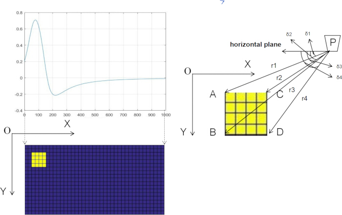
Figure 1: Schematic diagram of forward and inverse modeling processes. This figure illustrates the core workflow of magnetic anomaly forward and inverse modeling. In the forward process, a known subsurface geological model is used as input, and magnetic anomaly data at observation points are derived based on physical laws. In the inverse process, observed magnetic anomaly data are input into a convolutional neural network (CNN) to infer subsurface model parameters such as magnetization distribution and structural geometry. Please click here to view a larger version of this figure.
Forward modeling
Magnetic anomaly forward modeling is primarily used to calculate the response of subsurface models within a magnetic field. This process relies on the assumed distribution of magnetization within geological bodies and derives magnetic anomaly data at the surface or other observation points through physical equations. In forward modeling, the magnetic anomaly data correspond to the magnetization intensity. By comparing the simulated results with the actual subsurface structure model, the rationality of the forward modeling can be evaluated, which in turn helps improve inversion algorithms. The observation area for magnetic anomaly forward modeling is illustrated in Figure 2.
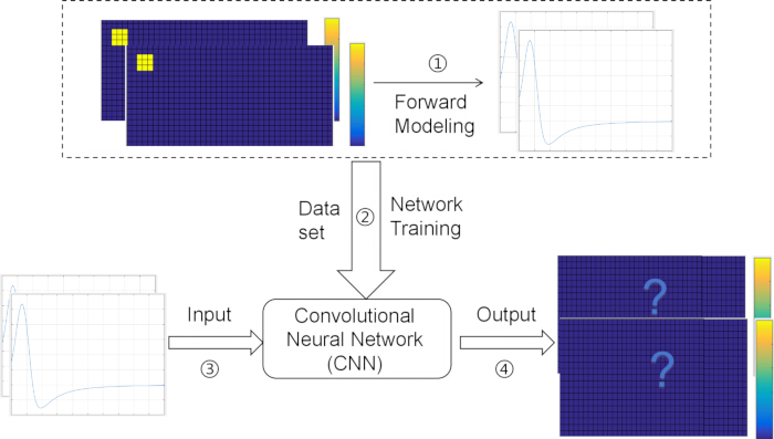
Figure 2: Schematic diagram of magnetic anomaly forward simulation. This figure presents the spatial layout of the observation region used in magnetic anomaly forward modeling. The horizontal plane and X-axis direction are indicated, and the subsurface domain is divided into multiple rectangular geological units. "Point P" represents a surface observation location. This diagram provides a visual explanation of the physical spatial relationship between grid cells and observation points, thereby supporting the theoretical interpretation of the forward modeling equation. Please click here to view a larger version of this figure.
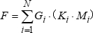
The subsurface space is divided into multiple square geological bodies, with point P representing a surface observation point. The forward modeling equation of magnetic anomalies describes the relationship between the magnetization intensity of the geological bodies and the observed magnetic anomaly, as shown in Equation (1):
 (1)
(1)
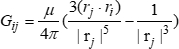
Here, F denotes the magnetic anomaly, typically represented as a column vector containing values from multiple observation points. Gi is the magnetic anomaly kernel matrix, where each element represents the contribution of the i-th grid cell to the magnetic field at the observation point. Ki is the magnetic susceptibility of the i-th grid cell, and Mi is its magnetization intensity. The computation of the kernel matrix generally depends on the spatial relationship between observation points and each grid cell. A commonly used approach is based on the magnetic dipole model, as shown in Equation (2):
 (2)
(2)
Here, Gij represents the magnetic field contribution from the j-th grid cell to the i-th observation point. µ denotes the magnetic permeability of free space. rj is the distance vector from the j-th grid cell to the i-th observation point, and | rj | is the magnitude of that distance.
Data preparation
In this study, 101 observation points were linearly arranged along a single survey line on the surface, with a uniform spacing of 10 m and an observation height of 0.3 m. The subsurface was discretized into a 20 × 40 grid, with each cell measuring 25 m × 25 m, and the magnetic declination and inclination angles were set to 90° and 60°, respectively. To simulate different geological structures, three types of synthetic subsurface models were constructed, all based on the aforementioned 20 × 40 grid. Values were assigned sequentially from left to right (columns 1→40) and from top to bottom (rows 1→20): the regular model consisted of 3 × 3 rectangular anomaly bodies (e.g., columns 10-12, rows 5-7) with a fixed magnetization of 5 A/m or 10 A/m; the complex model contained two trapezoidal anomaly bodies of different sizes (e.g., a large trapezoid in columns 8-15, rows 4-8, and a small trapezoid in columns 20-25, rows 6-9) with magnetizations of 5 A/m or 10 A/m; the random model was generated by selecting a central cell (e.g., column 20, row 10) and performing a random walk along columns and rows to create an anomaly region of 13-16 contiguous cells, with an overall magnetization of 5 A/m or 10 A/m. Fifteen, twenty, and thirty-two base structures were defined for the regular, complex, and random models, respectively, resulting in a total of 15 × 60 + 20 × 60 + 32 × 60 = 4020 training samples. Each model was sequentially assigned values, and its corresponding magnetic anomaly data was generated via forward modeling. The resulting dataset was split into training and testing sets at an 8:2 ratio, which were used for network training and performance evaluation, respectively. The specific forward modeling setup is illustrated in Table 1.
| Model | Model size |
| Regular Model | 3×6, 4×4 |
| Complex Model | double8×4, double trapezoid |
| Random Model | step size of 13, 16 random model |
Table 1: Setting of the model.
Network architecture
This study proposes an end-to-end magnetic anomaly inversion model constructed using a one-dimensional convolutional neural network (1D-CNN). The architectural design is inspired by the "deep convolutional stacking" paradigm of VGG networks and is further enhanced with an integrated attention mechanism. The objective is to achieve an efficient and accurate mapping from one-dimensional magnetic anomaly signals to the two-dimensional subsurface magnetization distribution. The overall network consists of five major components: input and data adaptation, feature-extraction backbone, CBAM attention modules, feature flattening, and fully connected layers.
Input layer and data adaptation
The input layer receives one-dimensional magnetic anomaly data, with its dimensionality strictly defined by the observation configuration. In the synthetic survey setup, 101 observation points are deployed at the surface with a 10 m spacing and an elevation of 0.3 m. Accordingly, the input dimension is defined as 1 × 101, where a single channel represents 101 magnetic anomaly amplitudes corresponding to the observation points.
In data preprocessing, 10% Gaussian white noise is added to emulate realistic observational disturbances. The signals are then normalized to the [0, 1] range using Min-Max scaling. This normalization alleviates dimensional inconsistency, stabilizes data distribution during training, and prevents biased parameter updates arising from magnitude discrepancies.
Feature extraction backbone
The feature-extraction backbone comprises 14 layers organized around repeated "Conv1d + BatchNorm + ReLU'' modules, interleaved with max-pooling operations for dimensionality reduction and multi-scale feature fusion. The backbone is grouped into four stages with progressively increasing channel depth.
Stage I (Basic feature extraction)
This stage includes three layers (Layer1-Layer3), producing 64-channel feature maps.
Layer1: A Conv1d layer with kernel size 3 (channels 1→64), followed by batch normalization and ReLU. Input size: 1×101; output: 64 × 101.
Layer2: Same configuration (64→64).
Layer3: MaxPooling1d with kernel size 2, reducing feature length from 101 to 50, yielding 64×50 feature maps.
Stage II (Mid-scale feature extraction)
This stage contains four layers (Layer4-Layer7), outputting 128 channels.
Layer4-Layer5: Conv1d layers increasing channels from 64 to 128; output size: 128 × 50.
Layer6: A CBAM module (see Section 3).
Layer7: MaxPooling1d reducing feature length to 25, giving 128 × 25 maps.
Stage III (Complex feature representation)
This stage also contains four layers (Layer8-Layer11), producing 256 channels.
Layer8-Layer9: Conv1d layers increasing channels from 128 to 256, output: 256 × 25.
Layer10: A second CBAM module.
Layer11: MaxPooling1d reducing length to 12, generating 256 × 12 maps.
Stage IV (Deep feature refinement)
This stage includes three layers (Layer12-Layer14), outputting 512 channels.
Layer12-Layer13: Conv1d layers increasing channels from 256 to 512.
Layer14: Final pooling reduces the feature length from 12 to 6, producing the deep 512 × 6 feature representation.
CBAM attention modules
The Convolutional Block Attention Module (CBAM) is strategically embedded after the 128-channel stage (Layer6) and the 256-channel stage (Layer10). It enhances the network's ability to focus on key anomaly-related features via channel and spatial attention mechanisms.
Channel attention submodule
Global max pooling and global average pooling are applied to the input feature map to produce two one-dimensional channel descriptors. After concatenation, the descriptors are passed through a fully connected layer with 32 neurons (ReLU activation), followed by another fully connected layer that outputs the channel-wise attention weights. These weights modulate the input features via element-wise multiplication, amplifying channels that contribute significantly to the magnetic anomaly inversion.
Spatial attention submodule
For the channel-refined feature map, channel-wise average pooling is performed, followed by a 1D convolution with kernel size 3 to generate the spatial attention weights. Element-wise multiplication with the input feature map enables the model to selectively emphasize spatial regions relevant to magnetic anomalies while effectively suppressing noise.
Feature flattening and fully connected layers
This module maps the extracted deep features to the final prediction domain.
Feature Flattening (Layer15): Converts the 512×6 feature map into a 3,072-dimensional feature vector.
Fully Connected Layer 1 (Layer16): Consists of 1,024 neurons with ReLU activation and Dropout regularization to mitigate overfitting. This layer integrates high-level features and projects them into a magnetization-oriented regression space.
Output Layer (Layer17): Contains 800 neurons corresponding to the 20×40 discretized subsurface grid. It outputs an 800-dimensional vector representing the estimated magnetization intensity of each grid cell, thereby completing the end-to-end inversion mapping.
Training Hyperparameters
To ensure stable and optimal training, the following hyperparameters are used: the Adam optimizer with an initial learning rate of 0.001; batch size of 32; and a total of 2,000 training epochs. Weight parameters of all Conv1d and fully connected layers are initialized using the He normal distribution, and all bias terms are initialized to zero.
Detailed network parameters are listed in Table 2.
| Layer | Operation Type | Input Size | Output Size | Kernel/Pool Size | Channels (in→out) |
| 1 | Conv1d + BatchNorm + ReLU | 1×101 | 64×101 | 3 | 1 → 64 |
| 2 | Conv1d + BatchNorm + ReLU | 64×101 | 64×101 | 3 | 64 → 64 |
| 3 | MaxPooling1d | 64×101 | 64×50 | 2 | |
| 4 | Conv1d + BatchNorm + ReLU | 64×50 | 128×50 | 3 | 64 → 128 |
| 5 | Conv1d + BatchNorm + ReLU | 128×50 | 128×50 | 3 | 128 → 128 |
| 6 | CBAM Module | 128×50 | 128×50 | ||
| 7 | MaxPooling1d | 128×50 | 128×25 | 2 | |
| 8 | Conv1d + BatchNorm + ReLU | 128×25 | 256×25 | 3 | 128 → 256 |
| 9 | Conv1d + BatchNorm + ReLU | 256×25 | 256×25 | 3 | 256 → 256 |
| 10 | CBAM Module | 256×25 | 256×25 | ||
| 11 | MaxPooling1d | 256×25 | 256×12 | ||
| 12 | Conv1d + BatchNorm + ReLU | 256×12 | 512×12 | 3 | 256 → 512 |
| 13 | Conv1d + BatchNorm + ReLU | 512×12 | 512×12 | 3 | 512 → 512 |
| 14 | MaxPooling1d | 512×12 | 512×6 | ||
| 15 | Flatten | 512×6 | 3072×1 | ||
| 16 | Fully Connected + ReLU + Dropout | 3072×1 | 1024×1 | 3072 → 1024 | |
| 17 | Fully Connected (Output) | 1024×1 | 800×1 | 1024 → 800 |
Table 2: Network Architecture Configuration.
Loss function
The essence of magnetic anomaly inversion lies in "inferring the subsurface model (cause) from the observed data (effect)." However, this process is inherently nonlinear and non-unique. Consequently, a network trained solely through conventional data-fitting losses may yield magnetization models that are numerically close to the ground truth yet physically implausible. To address this issue, the loss function in this study is designed to simultaneously achieve two objectives: (1) ensuring numerical agreement between the predicted and true magnetization parameters (data fitting), and (2) enforcing physical consistency so that the predicted results obey the governing laws of magnetic forward modeling (physics constraint).
Accordingly, the loss function is explicitly composed of two components:
Data misfit term: A mean squared error (MSE) term is used to quantify the discrepancy between the predicted and true subsurface magnetization parameters, ensuring the fundamental data-fitting capability of the network.
Physics-consistency constraint term: Derived from magnetic dipole forward modeling, this term measures the difference between the theoretical magnetic anomaly generated by the predicted magnetization and the observed magnetic anomaly. It ensures that the predicted model adheres to geophysical principles.
The two components are combined through weighted integration to form the total loss, establishing a closed loop of "data fitting + physical validation" and effectively avoiding the drawbacks associated with using a single loss term.
Mean squared error loss
The MSE loss measures the discrepancy between the model's predictions and the ground truth values. It calculates the average of the squared differences between predicted and true values, quantifying the error in each prediction task. For each branch (gravity anomaly and magnetic anomaly), the MSE loss is computed separately, representing the model's error on that specific task. The mean squared error loss function is expressed as Equation (3):
 (3)
(3)
Physics-based constraint loss
To prevent the inversion of magnetic anomalies from producing results that are "numerically close to the true values but physically infeasible" when relying solely on MSE, this study introduces a physics-consistency constraint based on the magnetic dipole forward model into the loss function. The predicted subsurface magnetization parameters are mapped through the forward kernel matrix to compute the corresponding theoretical magnetic anomalies, which are then compared with the observed data to directly assess the physical plausibility of the inversion results. This constraint effectively penalizes predictions that, although numerically close to the true values, fail to reproduce the observed anomalies when forward modeled, guiding the network to learn the physically consistent mapping from "subsurface magnetization → surface magnetic anomalies." To jointly optimize numerical accuracy and physical consistency, the total loss function combines the MSE data loss with the physics-consistency constraint in a weighted manner, ensuring that the model not only minimizes the difference between predicted and true magnetization values but also produces outputs that are physically consistent with the observations. Through this integrated mechanism, the physics-consistency constraint plays a crucial role in suppressing noise effects, mitigating non-uniqueness issues, enhancing inversion stability and generalization, and ultimately ensuring that the predicted magnetization distributions are both geophysically sound and practically applicable.. The physics-based constraint loss function is expressed as Equation (4):
 (4)
(4)
The final loss function is a weighted sum of the loss functions for gravity anomaly and magnetic anomaly, with each loss function comprising both the MSE loss and the physics-based constraint loss. The total loss function is expressed as Equation (5):
 (5)
(5)
Here, yltrue denotes the true magnetic anomaly data, predl represents the model's predicted magnetic anomaly, and Amat is the magnetic field kernel matrix.
Access restricted. Please log in or start a trial to view this content.
Results
Simulation experiments
Inversion results on the test set
The model is first trained on the training set and then evaluated on the test set, during which the prediction results on the test set are saved. To accelerate network convergence, appropriate hyperparameters are configured, as detailed in Table 3. After multiple training iterations, the loss curve stabilizes around epoch 1900; therefore, the total number of training epochs is set to...
Access restricted. Please log in or start a trial to view this content.
Discussion
This study proposes a magnetic anomaly inversion method that integrates the Convolutional Block Attention Module (CBAM) with physical consistency constraints to effectively address the common challenges of nonlinearity and non-uniqueness in geophysical inversion. By incorporating CBAM, the network can adaptively focus on critical channels and spatial regions, thereby significantly improving boundary resolution and reconstruction accuracy for complex subsurface structures and alleviating issues such as boundary blurring a...
Access restricted. Please log in or start a trial to view this content.
Disclosures
All authors confirm that they have no competing financial interests (including but not limited to grants, patents, consulting fees, stock holdings) or other personal, professional, or institutional conflicts of interest that could inappropriately influence the results or interpretation of this study.
Acknowledgements
This research was funded by the Chengde City Sustainable Development Project "Research and Application of a Knowledge Graph-Based College Student Employment System" (Project No. 202305B032) and projects from the Chengde Science and Technology Bureau (Project Nos. 202501A038 and 202305B032).
Access restricted. Please log in or start a trial to view this content.
Materials
| Name | Company | Catalog Number | Comments |
|---|---|---|---|
| Anaconda3 | Anaconda | https://mirrors.tuna.tsinghua.edu.cn/anaconda/archive/ | |
| MATLAB 2016b | MathWorks | https://www.mathworks.com/ | |
| Python3.7 | Python.org | https://www.python.org/downloads/release/python-370/ | |
| TensorFlow2.0 | https://tensorflow.google.cn/install | ||
| Windows10 | Microsoft | https://www.microsoft.com/zh-cn/software-download/windows10 |
References
- Liu, S., et al. Ant colony optimisation inversion of surface and borehole magnetic data under lithological constraints. J Appl Geophys. 112, 115-128 (2015).
- Biswas, A., Acharya, T. A very fast simulated annealing method for inversion of magnetic anomaly over semi-infinite vertical rod-type structure. Model Earth Syst Environ. 2 (4), 1-10 (2016).
- Constable, S. C., Parker, R. L., Constable, C. G. Occam's inversion: A practical algorithm for generating smooth models from electromagnetic sounding data. Geophysics. 52 (3), 289-300 (1987).
- Portniaguine, O., Zhdanov, M. S. Focusing geophysical inversion images. Geophysics. 64 (3), 874-887 (1999).
- Zhdanov, M. S., Fang, S., Hursán, G. Electromagnetic inversion using quasi-linear approximation. Geophysics. 65 (5), 1501-1513 (2000).
- Zhang, L., Koyama, T., Utada, H., Yu, P., Wang, J. A regularized three-dimensional magnetotelluric inversion with a minimum gradient support constraint. Geophys J Int. 189 (1), 296-316 (2012).
- Xiang, Y., Yu, P., Zhang, L., Feng, S., Utada, H. Regularized magnetotelluric inversion based on a minimum support gradient stabilizing functional. Earth Planets Space. 69 (1), 158(2017).
- Last, B., Kubik, K. Compact gravity inversion. Geophysics. 48 (6), 713-721 (1983).
- Chen, Z., Zhang, X., Chen, Z. Combined compact and smooth inversion for gravity and gravity gradiometry data. IEEE Trans Geosci Remote Sens. 60, 1-10 (2021).
- Nazari, H., Esmailzadeh, M., Hajizadeh, F., Joulidehsar, F. Three-dimensional inversion of magnetic data using compaction constraint: A case study-Sharif Kandi, West Iran. Arab J Geosci. 14 (14), 1391(2021).
- Utsugi, M. 3-D inversion of magnetic data based on the L1-L2 norm regularization. Earth Planets Space. 71 (1), 73(2019).
- Li, Y., Oldenburg, D. W. 3-D inversion of magnetic data. Geophysics. 61 (2), 394-408 (1996).
- Pilkington, M. 3-D magnetic imaging using conjugate gradients. Geophysics. 62 (4), 1132-1142 (1997).
- Minami, T., Utsugi, M., Utada, H., Kagiyama, T., Inoue, H. Temporal variation in the resistivity structure of the first Nakadake crater, Aso volcano, Japan, during the magmatic eruptions from November 2014 to May 2015, as inferred by the active electromagnetic monitoring system. Earth Planets Space. 70 (1), 138(2018).
- Bai, Z., et al. Joint gravity and magnetic inversion using CNNs' deep learning. Remote Sens. 16 (7), 1115(2024).
- Gao, M., Wang, J., Li, S. 3D inversion of gravity and magnetic data using deep residual networks. IEEE Trans Geosci Remote Sens. 58 (9), 6554-6566 (2020).
- Hubbert, M. K. Entrapment of petroleum under hydrodynamic conditions. AAPG Bull. 37 (8), 1954-2026 (1953).
- Liu, S., Hu, X., Liu, T. A stochastic inversion method for potential field data: Ant colony optimization. Pure Appl Geophys. 171 (7), 1531-1555 (2014).
- Dao, T., Fu, D., Ermon, S., Rudra, A., Ré, C. FlashAttention: Fast and memory-efficient exact attention with IO-awareness. Adv Neural Inf Process Syst. 35, 16344-16359 (2022).
- Goodfellow, I., et al. Generative adversarial networks. Commun ACM. 63 (11), 139-144 (2020).
Access restricted. Please log in or start a trial to view this content.