Automated Sample Preparation for the Multiplexed Analysis of Single-Cell Histone Post-Translational Modifications (sc-hPTM2)

Summary

Here, we present a protocol to automate single-cell histone post-translational modification analysis using an isotopic two-plex labeling strategy and ArgC digestion. This workflow enables quantitative, reproducible, and high-sensitivity profiling of chromatin heterogeneity and epigenetic responses at single-cell resolution.

Abstract

Histone post-translational modifications (hPTMs) are central regulators of chromatin organization and gene expression. Their dysregulation is implicated in development, cancer, and aging. While mass spectrometry is the method of choice to study hPTMs, most protocols are designed for bulk samples and cannot resolve cell-to-cell variability. Extending histone PTM analysis to the single-cell level is therefore essential but technically challenging, as histones are low in abundance, lysine-rich, and heavily modified.

Here, we describe an automated single-cell proteomics workflow for histone PTM analysis using nano liquid handling. The system enables nanoliter-scale processing of individual cells with minimal handling and high reproducibility. The workflow includes digestion with ArgC Ultra protease, which cleaves at arginine residues and avoids the need for lysine-blocking derivatization steps typically required in histone proteomics. To enable quantitative comparison between conditions, we apply a two-plex labeling strategy with propionic anhydride and its deuterated analogue, propionic anhydride-d10. This combination of automated sample preparation, isotopic multiplexing, and ArgC Ultra digestion results in a streamlined and sensitive protocol for single-cell histone PTM analysis.

The method allows for the investigation of chromatin heterogeneity and the effects of epigenetic perturbations at single-cell resolution. To demonstrate the workflow, we generated spheroids from HepG2/C3A hepatocellular carcinoma cells and treated them with sodium butyrate, a histone deacetylase inhibitor that induces hyperacetylation.

Introduction

Histones are the protein components of nucleosomes, the repeating units of chromatin. Their N-terminal tails are rich in lysine and arginine residues and are highly regulated by post-translational modifications (PTMs), such as acetylation, methylation, and phosphorylation. These modifications influence DNA accessibility and thereby control processes including transcription, replication, and repair. Altered histone PTM patterns are strongly associated with disease states, from cancer to neurodegeneration and aging^1,2. For this reason, histone PTM analysis has become of great interest in epigenetics and proteomics research. Mass spectrometry (MS) provides site-specific and quantitative analysis of histone modifications, but histones present unique analytical challenges. Their amino acid composition, multiple modification sites, and complex combinatorial patterns make them more difficult to analyze than typical proteins. Established protocols rely on chemical derivatization to block lysine residues before digestion, improving peptide recovery and chromatographic performance³. While effective in bulk analyses, these multi-step derivatization protocols can introduce losses that are problematic for single-cell inputs. Single-cell analysis is increasingly important because biological systems are inherently heterogeneous. Bulk histone analyses average signals across many cells and thus fail to capture this variability. Subpopulations of cells may differ in their chromatin states, and these differences can drive development, cellular reprogramming, or drug responses^4,5.

Here, we present an automated sample preparation method for the multiplexed single-cell histone PTM analysis (sc-hPTM2). This method relies on the CellenONE system, which allows precise dispensing of individual cells and nanoliter-scale reagents in an automated fashion. This method is a variation on the nano proteomic sample preparation (nPOP) method, which first introduced the use of droplet preparation on a glass slide⁶. The nPOP platform has advanced automated single-cell proteomics, yet its standard tryptic digestion protocol is suboptimal for histones due to their high lysine content and extensive modification density. Here, we adapted the CellenONE system to incorporate the gold-standard histone derivatization with propionic anhydride and introduced isotopic labeling, enabling accurate and comprehensive quantification of histone post-translational modifications at single-cell resolution. Specifically, we simplify the protocol by using ArgC Ultra protease for protein digestion. Unlike trypsin, ArgC cleaves only at arginine residues and does not require lysine blocking. This eliminates the need for a two-step derivatization strategy, streamlining the protocol. In addition, the method incorporates a two-plex isotopic labeling scheme using propionic anhydride and propionic anhydride-d10, allowing for 2 cells to be analyzed simultaneously^7,3. Following digestion and labeling, single-cell samples are recovered and analyzed by liquid chromatography-mass spectrometry (LC-MS)/MS using data-independent acquisition (DIA). In our hands, this method has been shown to provide an increase in both sensitivity and reproducibility for quantification of histone PTMs as compared to the previous version of this method⁸.

To demonstrate the method, we profiled single-cell histone PTM dynamics in spheroids derived from HepG2/C3A hepatocellular carcinoma cells. We treated these spheroids with sodium butyrate, a well-characterized histone deacetylase inhibitor that increases histone acetylation and serves as a benchmark for probing chromatin regulation^9,10. By comparing control and sodium butyrate-treated spheroids at single-cell resolution, we demonstrate a proof of principle of representative results, highlighting the potential for broader applications in chromatin biology and cancer epigenetics. Notably, for the protocol, we refer to a prior publication describing growth and treatment of 3D spheroids¹⁰, acquisition of histone peptides in mass spectrometry¹¹, and data analysis using the software EpiProfile¹².

Protocol

1. Buffers and reagents

1. Cell growth media for HepG2/C3A cells: Prepare Dulbecco's Modified Eagle's Medium (DMEM, 4.5g/L glucose) containing 10% fetal bovine serum (FBS), non-essential amino acids (1% v/v), L-glutamine (1% v/v), and penicillin/streptomycin (0.5% v/v). Growth media is stored at 4 °C.
2. Master mix: Prepare ArgC Ultra 60 ng/µL, HEPES 6 mM, n -dodecyl-β-D-maltoside (DDM) 0.03%, Dithiothreitol (DTT) 10 mM in LC-MS grade water.
3. HA solution: Prepare 1% (v/v) hydroxylamine in LC-MS grade water.
4. Wash solution: Prepare 10 mL of a 50:50 acetonitrile/water mixture containing 0.1% (w/w) formic acid (all LC-MS grade).
5. Mobile Phase A (MPA) - 0.1% formic acid: Add 1 mL of concentrated formic acid to 999 mL of HPLC-grade water and mix well.
6. Mobile Phase B (MPB) - 80% HPLC-grade acetonitrile + 0.1% formic acid: Add 800 mL of HPLC-grade acetonitrile to 199 mL of HPLC-grade water. Next, add 1 mL of concentrated formic acid to this solution and mix.

2. Spheroids preparation

1. For the spheroids preparation, refer to Stransky S et al.¹¹.
2. Culture HepG2/C3A hepatocellular carcinoma cells in a rotating three-dimensional (3D) bioreactor for 5-7 days to promote uniform spheroid formation until reaching ~400-600 µm diameter. Use DMEM supplemented with 10% FBS, 1% non-essential amino acids, 1% L-glutamine, and 0.5% penicillin/streptomycin. Maintain spheroids at 37 °C and 5% CO₂ until treatment.
   NOTE: Figure 1A represents the equipment used to prepare the spheroids in the reference paper.

3. Cell culture and treatment

1. Put ~10 spheroids in a tissue-culture 6-well plate containing 2 mL of growth media.
2. Incubate the cells at 37 °C in a humidified 5% CO₂ incubator.
3. Treat the spheroids for 24 h with 5 mM sodium butyrate or add the same volume of water for the control (Figure 1B).

4. Cell isolation and single-cell suspension preparation

1. After 24 h of treatment, incubate the cells with 1 mL of trypLE at 37 °C for 3-5 min.
2. Gently pipette up and down until the spheroid breaks apart and single cells are obtained.
3. Collect the cells in a 15 mL tube and wash, diluting up to 10 mL with ice-cold 1x PBS, centrifuge at 500 g for 5 min at 4 °C, and aspirate the supernatant.
4. Resuspend the cells in 1 mL of ice-cold 1x PBS and add Sytox green dead cell stain with a final concentration of 1 µM.
5. Incubate the cell with Sytox green for 20 min on ice in a dark environment.
6. Wash the cell with 10 mL of ice-cold 1x PBS, centrifuge at 500 g for 5 min at 4 °C, and aspirate the supernatant.
7. Resuspend the cells in 1 mL of ice-cold 1x PBS and add paraformaldehyde (PFA) with a final concentration of 0.5%.
8. Incubate the cell with PFA for 15 min on ice.
   NOTE: While Sytox green is typically not compatible with fixation due to membrane permeabilization, for cells we have tested the proportion of Sytox green cells remains the same up to 8 h after fixation with no signs of histone protein leakage.
9. Wash the cell with 10 mL of ice-cold 1x PBS, centrifuge at 500 g for 5 min at 4 °C, and aspirate the supernatant.
10. Reconstitute the cells at a final concentration of 200-500 cells/μL.
    NOTE: For small cells that do not tend to deposit, a concentration of 500 cells/µL is recommended, while for large cells that tend to deposit, a concentration of 200 cells/µL is recommended. If the cell suspension is prone to aggregation, run it through a 40-μm strainer before aspiration to avoid nozzle clogging. If cells larger than 40 μm are of interest and probably present in a sample, a 70-μm strainer can be used instead to remove very large aggregates.
11. Store the cells on ice until loaded into the instrument for sorting.

5. Software connection and system initialization

1. Turn on the cellenONE system (Figure 2A), boot the control computer, launch the software, and open the v2.0-nPOP2 user workspace; all required field files and run templates for nPOP are pre-loaded there.
2. Make sure the instrument's chiller is switched on, then set the dew-point-chase value according to the internal temperature currently reported by the instrument.
3. Prime the system with PDC-70, coating-type 2 dispensing nozzles (Figure 2B) installed in slots 1 and 3, following the on-screen instructions.
4. Set each nozzle's pulse width and drive voltage to the values specified on the manufacturer's packaging.
   NOTE: Using two separate nozzles preserves dispensing consistency: one delivers the cell suspension, the other the reagents, so any debris adhering to a nozzle will not compromise subsequent drops. Employing both nozzles during the final collection step also accelerates sample recovery.
   1. (CRITICAL STEP) For maximal pick-up efficiency, the z-offset between the two nozzles should differ by <50 µm. Determine this by defining the optimal contact position for each nozzle and comparing the Z-height read-outs in the Nozzle Setup tab.
5. Fill the humidifier reservoir with de-ionised water up to the indicated fill line.

6. Pre-run configuration on the liquid handler

1. Select the quantity of glass slides (Figure 2C) to be prepared. This choice directly defines the total number of cells planned to analyze.
2. For a 2-plex multiplexing scheme (Figure 3A), load a single slide with 320 cells.

7. Dispensing a dimethyl sulfoxide (DMSO) "moat" around slide edges

NOTE: Figure 3B represents the steps for preparing the samples in the cellenONE starting from the moat of DMSO. As an additional prevention against droplet evaporation, DMSO is dispensed along the edges of the slides.

1. In the Main tab, select the run to 0_Dispense_DMSO_Moat.
2. Go to Target Setup tab, load the DMSO_Moat.fld file from the appropriate scheme folder, and set No. of Fields to Y, matching the number of slides planned to process.
3. Aliquot 150 µL of LC-MS-grade DMSO into a new PCR tube and place it into position 2 of the CellenWASH station with the tube cap facing the instrument door.
4. Open the Run tab and click Start Run. The system will aspirate 10 µL of DMSO and pause for user confirmation of the droplet stability. Fire three autodrop test droplets (Figure 4A); if all three are perfectly formed, click Continue Run.
5. After dispensing, the nozzles flush automatically, and the instrument captures images across all slides for quality control. Review the images to verify a uniform DMSO droplet on every slide and to check for missing or off-target droplets (Figure 4B).

8. DMSO dispense

1. In the Main tab, select the run to 1_Dispense_DMSO.
2. Open Target Setup tab, import the field file DMSO.fld (Figure 4C) from the appropriate scheme directory, and set Number of Fields to Y, matching the slide count you intend to process.
3. Aliquot 150 µL of LC-MS-grade DMSO into a new PCR tube and place it into position 2 of the CellenWASH station with the tube cap facing the instrument door.
4. Open the Run tab and click Start Run. The system will aspirate 10 µL of DMSO and pause for user confirmation of the droplet stability. Fire three autodrop test droplets; if all three are perfectly formed, click Continue Run.
5. When dispensing finishes, the software automatically flushes the nozzles and captures images across every slide for quality assurance. Review the images to verify a uniform DMSO droplet on every slide and to check for missing or off-target droplets.

9. Cell dispense

1. In the Main tab, select the run to 2_Dispense_Cells.
2. In Target Setup tab, open the Cells Field Files sub-folder of the chosen multiplexing-scheme directory.
3. Because the experiment involves two conditions, pick the field file that matches the sample that is about to sort-either CellType_A.fld or CellType_B.fld.
4. After the file loads, set Number of Fields to Y, so it equals the total slide count for this run.
5. Degas the cell suspension from step 4.11 with a vacuum pump for 10 min on ice.
6. Transfer 150 µL of the prepared cell suspension into a clean CellenVIAL, then place the vial in slot 1 of the CellenWASH carousel with its cap pointing toward the instrument door.
7. Go to the Nozzle Setup tab > Do Task and execute Take10ul_CellenVIAL_nozzle1 to aspirate the sample from the vial.
8. Staying in the Nozzle Setup tab, launch the cell-dispensing viewer (Figure 5A) and run the mapping routine to define the ejection zone and gate objects based on size and elongation. The single-cell isolation parameters shown in Figure 5A correspond to the exact settings used for dispensing HepG2/C3A cells dissociated from spheroids.
9. Then activate the fluorescence mode by selecting T > F. Set the selection mode to negative. Increase the isolation parameter range for size and intensity from the minimum to the maximum values to ensure that no dead cells are isolated.
10. Verify with the mapping parameters, open the Run tab, and click Start Run, then follow the software prompts. When dispensing ends, the instrument will automatically flush the nozzles and capture slide images for review of droplet placement and uniformity.
    NOTE: During cell sorting, images are taken of each individual cell that is isolated during the run (Figure 5B).
11. After cell sorting finishes, close the dispensing window.
12. Keep any leftover cell suspension on ice until section 9 is over; the surplus can be used later for bulk samples, empirical-library construction, or additional validation studies.

10. Digestion master mix dispense

1. In the Main tab, select the run to 2_Dispense_Digest_10ulPickup.
2. Open the Target Setup tab, load Digest.fld from the appropriate multiplexing-scheme folder, and set Number of Fields to Y so it equals the slide count for this run.
3. Prepare a fresh digestion master mix and degas the solution with a vacuum pump for 10 min on ice (Master mix: ArgC Ultra 60 ng/µL, HEPES 6 mM, DDM 0.03%, DTT 10 mM in LC-MS grade water).
4. Pipette 20 µL of the master mix into a 384-well plate and place the plate inside the X1 system.
5. In the Run tab, click Start Run and follow the prompts. After the system aspirates the reagent, confirm droplet stability when prompted.
6. When dispensing finishes, the instrument automatically flushes the nozzles and photographs every slide; review the images to verify that each droplet received the digestion mix uniformly.
7. Incubate the slides overnight for digestion, maintaining the specified humidity and dew-point settings. Each droplet contains ~13.5 nL of digestion mix. Carry out digestion overnight at ~75 % relative humidity, with the dew point maintained 1-2 °C below the chamber temperature to prevent droplet evaporation.

11. Incubation overnight

1. In the Main tab, choose the run to 4_Incubation_16h.
2. Switch to the Run tab, click Start Run.
   NOTE: The instruments will take pictures of the slides every 30 min to monitor the condition of the droplets. If they dry out or swell during incubation, adjust the dew-point setting as needed.
3. When the incubation is done, a message will pop up saying that the incubation is completed.
   NOTE: Rapid digests (≤4 h) may be achievable with higher effective enzyme-to-substrate conditions; this was not evaluated here, so the validated condition remains 16 h.

12. Evaporation

NOTE: Before moving on to the labeling step, it is recommended to check the condition of the droplets to ensure that they are not too swollen with water, as water could interfere with the efficiency of labeling. For this purpose, the evaporation phase is recommended.

1. In the Main tab, choose the run to 5_Evaporation.
2. Go to File, Cooling Unit Control, and under the Dew Point Control set Fixed Control Temperature at 23 °C.
3. Switch to the Run tab, click Start Run. The drying will last for 5 min, and the instruments will automatically capture pictures of the slides after the drying.
4. Inspect the pictures; if the droplets are sufficiently dry, stop the run. If not, click continue and dry for another 5 min (Figure 6A).
5. At the end of the run, switch back to the previous Dew Point Control.

13. Labels dispense

1. In the Main tab, choose the run to 6_Dispense_PA_Labels.
2. Go to the Target Setup tab, load the Labels.fld file from the appropriate scheme folder, and set No. of Fields to Y, matching the number of slides planned to process.
3. Aliquot 150 µL of LC-MS-grade DMSO into slot 2 of the CellenWASH station.
4. Prepare a stock solution of the two labelling stocks for multiplexed histone derivatisation: 25% (v/v) propionic anhydride in DMSO and 25% (v/v) propionic anhydride-d₁₀ in DMSO.
   NOTE: Degas both solutions before transferring them to the plate to minimize bubble formation.
5. Dispense 20 µL of each labeling reagent into the designated wells of a 384-well plate and place the plate inside the X1 system. Each droplet receives ~10 nL of labeling reagent (25% propionic anhydride or 25% propionic anhydride-d₁₀ in DMSO).
6. Switch to the Run tab, click Start Run, and follow the prompts.
7. Allow the labels to react on-slide for 1 h.
8. After dispensing, the instrument automatically flushes the nozzles and photographs every slide. Review the images to confirm even distribution and correct droplet placement across all slides.

14. HA dispense

1. Prepare the HA solution and degas it before use.
2. Load the vial. Pipette 150 µL of the HA solution into a clean PCR tube, position it in CellenWASH slot 2, and orient the cap toward the instrument door.
3. Select the run profile. In the Main tab, choose 7_Dispense_Quench.
4. Configure the field file. Open the Target Setup tab, load HA.fld from the appropriate multiplexing-scheme folder, and set Number of Fields to Y so it equals the total slide count.
5. Start the run. Navigate to Run, click Start Run, and follow the on-screen instructions.
6. Incubate. Let the HA react on the slides for 30 min.
7. Verify dispensing. After completion, the system flushes the nozzles and captures images of each slide-review these images to confirm uniform droplet placement and volume.

15. Sample pick-up

1. Prepare the wash solution in the WashTray XL.
2. Set up the collection plate. Dispense 2 µL of 0.01% (w/w) DDM in LC-MS-grade water into every well of a fresh 384-well plate and place the plate inside the liquid handler.
3. Choose the pick-up run. In the Main tab, select the profile 8_Pickup_2plex.
4. Load the field file. Open the Target Setup tab, import Pick-up.fld from the correct multiplexing-scheme directory, and set Number of Fields to Y so it matches the slide count.
5. Execute the run. Switch to the Run tab, click Start Run, and follow the prompts. The instrument will collect each droplet, flush the nozzles, and image the slides for review to confirm that every sample has been retrieved.

16. Post-pickup processing

1. Seal the 384-well plate with adhesive foil and centrifuge briefly to bring droplets to the bottoms of the wells.
2. Remove the foil and dry the samples at low heat in a vacuum concentrator.
3. Seal the plate with adhesive foil and store the dried plate at -80 °C until ready for LC-MS/MS analysis.

17. Bulk samples preparation

1. Using the leftover suspension from section 9, spin down the cells and resuspend in 1x PBS to obtain a concentration of 2,000 cells/µL. This should be performed following the completion of section 10.
2. Thermal lysis: snap-freeze the remaining suspension at -80 °C for 10 min, then heat-shock at 90 °C for 10 min.
3. Allow the tube to cool back to room temperature.
4. Transfer 25 µL of the lysate to a PCR tube and add 5 µL of the previously prepared digestion mix.
5. Incubate overnight (≈ 16 h) at 37 °C in a thermal cycler.
6. Light-label derivatisation: add 5 µL of a fresh 25% (v/v) light label in acetonitrile and incubate for 1 h.
7. Reaction quench: add 5 µL of 1% (w/w) hydroxylamine (HA) solution and incubate for 30 min.
8. Dry the sample in a vacuum concentrator set to low heat, then store at -80 °C until ready for LC-MS/MS.

18. LC/MS setup and data acquisition

NOTE: To collect the data for this manuscript, a LC-MS\MS system setup with an Ion Optics 75 µm ID x 25 cm x 1.7 µm analytical column.

1. Prepare the mobile phases to run on the HPLC:
   Mobile Phase A (MPA): 0.1% formic acid in HPLC-grade water
   ​Mobile Phase B (MPB): 0.1% formic acid in HPLC-grade acetonitrile
2. Program the HPLC method for a 30-min active gradient: 5-23% MPB in 25.7 min, 23-35% MPB in 2.6 min and 35-45% MPB in 1.7 min, at a flow rate of 200 nL/min. Program the autosampler to resuspend the sample in 0.1% FA + 0.01% DDM for ‘dry’ pick up.
3. Set up the MS acquisition method to perform data-independent acquisition (DIA):
   NOTE: These settings are specific for a Thermo Exploris 480 equipped with FAIMS Pro Duo and may differ depending on your instrument. It is recommended to use those that are common for DIA single-cell proteomics with similar m/z ranges as described below.
   1. Set the MS to be a full scan from 300-1100 m/z with a resolution of 120,000, AGC target of 300%, maximum injection time of 246 ms, and FAIMS CV of -50 V.
   2. Set the MS/MS to be a DIA scan from 300-1100 m/z with a resolution of 60,000, isolation window of 50 m/z, HCD collision energy of 27%, first mass of 120 m/z, AGC target of 1000%, maximum injection time of 118 ms, and FAIMS CV of -50 V.
4. Remove the foil seal from the 384-well plate containing the single cells. Reconstitute the bulk sample at 100 cells/µL in 0.1% FA + 0.01% DDM and transfer 10 µL into an empty well, such as P24. Then, seal the plate with a pierceable rubber mat and load it into the autosampler.
5. Queue up runs: run first the bulk samples and then the sets of single cells.

19. Data analysis

1. Run the raw data with EpiProfile2.1 to get the output with the peptidoforms abundances for the cells labeled with propionic anhydride.
   NOTE: Samples must be acquired on a Thermo instrument in order to use EpiProfile 2.1 for data processing. This software extracts approximately 250 peptidoforms with its canonical version, but it is editable depending on the organism, additional modifications of interest, mutations, etc.¹².
2. Run the raw data with EpiProfile2.1_D5 to get the output with the peptidoforms abundances for the cells labeled with propionic anhydride-d10.
3. Perform the mapping linking the metadata with the Epiprofile outputs with the quantQC program.
4. Filter out failed samples by comparing with the blanks.
5. Filter out peptidoforms that are not in at least 50% of the samples.
6. Filter out peptidoforms whose signal of the single cell intensity is not greater than the 150% signal in blanks.
7. Obtain the results table (Figure 7A) and process the data further as needed.

Results

To demonstrate the application of our single-cell histone proteomics workflow using our system, we analyzed spheroids of HepG2/C3A cells treated with 5 mM sodium butyrate for 24 h. After LC-MS/MS acquisition, raw data were processed with EpiProfile for both light (propionic anhydride) and heavy (propionic anhydride-d10) labeling, obtaining normalized data representing the abundances of the peptides and histone marks. The QuantQC R package was then used to map the acquisition metadata of the liquid handler to the EpiProfile outputs in order to get the information of the peptides content and related abundance for each cell, then were filter out peptidoforms not consistently detected in at least 50% of the single cells, and excluded peptidoforms whose signal of the single cell intensity is not greater than the 150% signal in blanks. Data were subsequently normalized using a log(1+x) transformation to obtain the results table that is used for downstream analysis, which consists of a column with the various peptidoforms and columns for each individual cell with the abundances of the various identified peptidoforms.

Figure 7A shows a representative subset of the results table containing the first 20 histone H3 peptidoforms quantified. The values are expressed as relative abundances in control and sodium butyrate-treated conditions. This overview highlights how the workflow allows the detection of diverse PTM states at single-cell resolution, including methylation, acetylation, and combinatorial marks. For example, H3K9ac and H3K14ac both show increased relative abundance upon sodium butyrate treatment, consistent with the expected inhibition of histone deacetylases (HDACs). Similarly, histones co-modified with H3K9acK14ac appear even more enriched in the treated cells, reflecting the cooperative nature of acetylation marks in regulating chromatin accessibility.

Notably, results can be dissected into multiple layers. First, a good quality control is to ensure that an overall increase in total histone acetylation upon sodium butyrate exposure is observed (Figure 7B). Importantly, the treated cells display a broader error distribution compared to controls, reflecting the higher heterogeneity captured at the single-cell level. This illustrates how single-cell proteomics can reveal not only average shifts in PTM levels but also the variability across individual cells within a given population. Figure 7C aims to demonstrate that, when histones are cleaved into relatively long peptides, it is possible to quantify not only the relative abundance of single modifications, but also their co-occurrence frequency. In the example, the effect of sodium butyrate is mostly evident in the combinatorial acetylation state H3K9acK14ac, which is often associated with transcriptional activation. These patterns align with the effect of sodium butyrate and show the ability of our approach to detect biologically meaningful changes in histone PTMs at the single-cell scale.

To explore global differences, we performed PCA across all quantified peptidoforms (Figure 7D). Control and treated cells separated along the first principal component, which captured ~40% of the total variance. The wider dispersion of the sodium butyrate-treated cells indicates increased biological heterogeneity, consistent with variable acetylation responses among individual cells within the spheroids following HDAC inhibition.

These representative results demonstrate the efficiency and robustness of the workflow in capturing histone post-translational modifications at single-cell resolution and preserve information on cell-to-cell variability. By integrating sample preparation, acquisition, and computational analysis, this pipeline provides a practical and reproducible approach for profiling histone PTMs in single cells, making it suitable for broader applications in chromatin biology and drug-response studies.

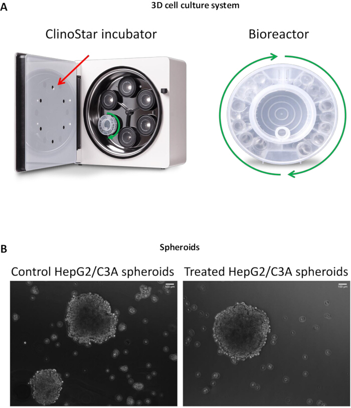
Figure 1: 3D culture system and spheroids. (A) 3D cell culture system. The bioreactor on the right is the device in which the cells are cultured. On the left is the incubator, which can hold up to 6 bioreactors and maintains a specific rotation speed, CO₂ level, and temperature. (B) HepG2/C3A spheroids during sodium butyratetreatment. The spheroids are cultured in 6-wells plate during the treatment with 5 mM of sodium butyrate for 24 h. Panel A has been modified with permission from https://celvivo.com/. Please click here to view a larger version of this figure.

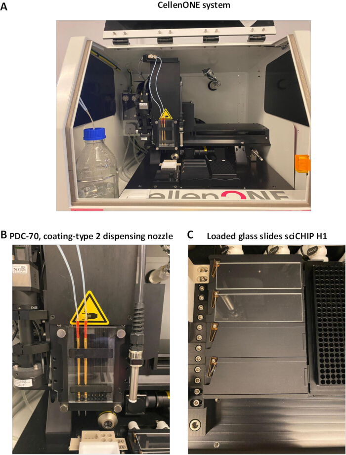
Figure 2: CellenONE instrument system. (A) Internal view of the instrument where sample preparation takes place. The figure shows the bottle containing milliQ water that feeds the instrument's liquid system, the nozzles involved in dispensing reagents and cells connected to the pumps, the glass slides loaded into the slide holder, the holder for the 384-well plate, and the cellenWASH station where the PCR tubes with reagents are placed. (B) PDC-70, coating-type 2 dispensing nozzles. The nozzles used during sample preparation are in positions 1 and 3. The nozzle in position 1 dispenses the cells, while the one in position 3 dispenses all the reagents used. The coated nozzles reduce cell and peptides sticking, useful for cell dispensing and optimal pick-up. Moreover, it gives a more reproducible droplet size. Compatible with all the reagents used in this protocol. (C) Glass slides sciCHIP H1 loaded. In the picture, there are two slides loaded in the slide holder that can hold up to 4 slides. The slides need to be very clean, flat, and aligned with the top right corner. Please click here to view a larger version of this figure.

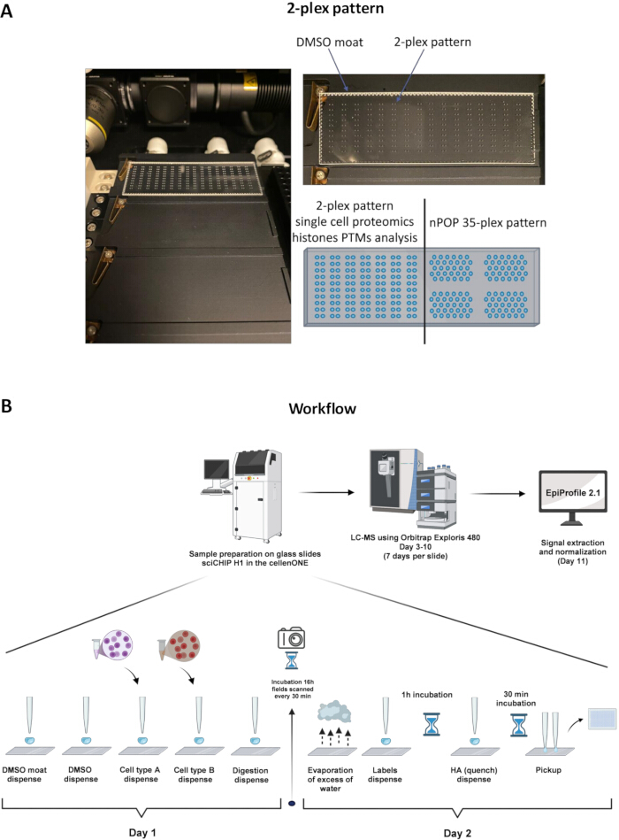
Figure 3: 2-plex pattern and workflow for sample preparation, data collection and data analysis. (A) Representation of the 2-plex pattern and DMSO moat. The figure shows the DMSO moat, which prevents excessive drying of the droplets during sample preparation, and the 2-plex pattern following DMSO dispensing. It also shows the difference between the 2-plex pattern described in this protocol and what is expected in an nPOP experiment with TMT 35-plex labeling. (B) Schematic overview of the experimental pipeline. Sample preparation takes place over two days: in the first part, DMSO, single cells, and the master mix for digestion are dispensed. The digestion is incubated overnight, during which photos of the droplets on the slides are taken every 30 min. In the second phase, after evaporation of any excess water that may have formed, labeling, quenching, and finally the pick-up of the cell sets in a 384-well plate are performed. Processed samples are analyzed by mass spectrometry, and the resulting data are subjected to computational analysis to obtain a quantitative profile of histone PTMs. Please click here to view a larger version of this figure.

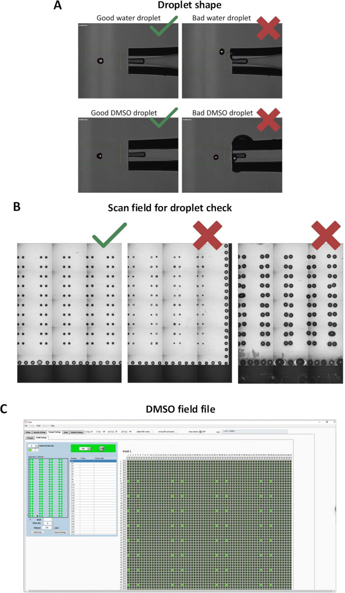
Figure 4: Accuracy of dispensed drops. (A) Images of autodrop test of the droplets. The first two images above show two autodrop test images in which the reagent is mainly composed of water. The first shows a correctly formed drop, while the second shows an incorrect drop that will need to be fixed before continuing with the preparation. The first two images below show two autodrop test images in which the reagent is mainly composed of DMSO. First, note how the DMSO appears transparent compared to water, and as in the previous images, one can see a correctly formed drop and an incorrect drop that will need to be corrected before continuing with the preparation. (B) Examples of fields scanned after dispensing. In the figure, the first image shows a successful dispensing in which the drops have the correct shape. The second shows drops that are too dry and therefore reduced in size, while the last shows drops that are too swollen and increased in size, where some have even merged. (C) Image of a field file used for DMSO dispensing. Representation of a file in which the position of the drops, the volume, the probe from which the reagent is dispensed, and the nozzle used are determined. Please click here to view a larger version of this figure.

Figure 5: Types of visualizations during cell sorting. (A) CellenONE dispensing viewer. The figure shows the window that opens during cell sorting. Cells can be isolated based on transmission, which mainly determines size and elongation, while fluorescence is used to isolate live cells based on intensity, following the use of dyes such as SytoxGreen, which tag dead cells. The bottom part shows the cells plotted during analysis and isolation, depending on whether they are detected, isolated, or not. (B) Visualization of cell isolation based on transmission. The single cell is about to be isolated based on characteristics determined after mapping and analysis. Cells sticking to the glass tip outside the nozzle following sample aspiration are noted; these do not interfere with isolation, as they are indicated as background. Please click here to view a larger version of this figure.

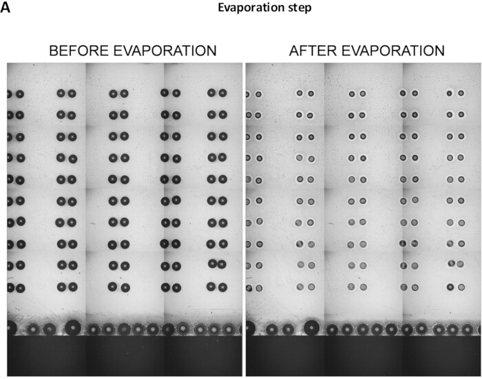
Figure 6: Evaporation step. The first image shows a scan field after overnight incubation of the digestion, in which the droplets are slightly swollen due to water collected from the humidity present in the system. The excess water is evaporated so that it does not interfere with the efficiency of labeling. The second image shows a scan field of droplets after the evaporation step, ready for the next labeling step. Please click here to view a larger version of this figure.

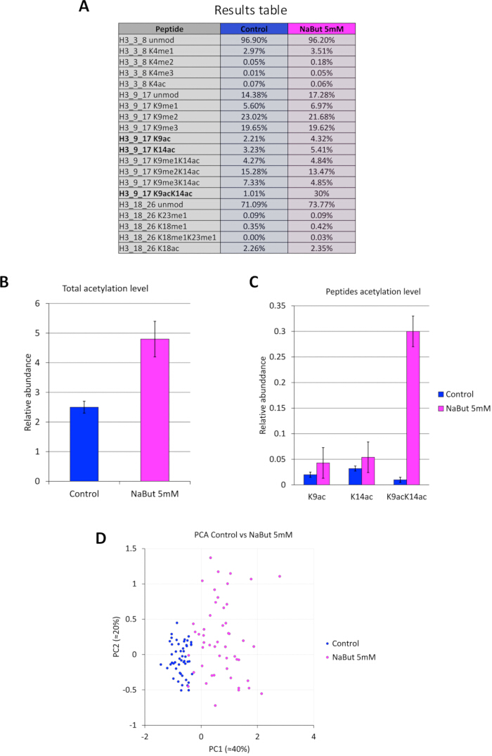
Figure 7: Data analysis of histone PTMs at a single cell level. (A) Table list of identified peptides with post-transcriptional modification sites and relative abundance of each of them in both conditions, control and treated. In this results table, every column corresponds to a cell. (B) Relative abundance of acetylation in the total of cells. (C) Relative abundance of acetylation for representative peptides of single and combinatorial modifications. (D) Principal component analysis (PCA) was performed to show the separation of the two cell groups and the heterogeneity of the treated cells. Please click here to view a larger version of this figure.

Discussion

The ability to measure histone post-translational modifications at the single-cell level represents a critical step toward understanding the true heterogeneity of chromatin regulation. Traditional bulk methods have provided invaluable insights into the average distribution of hPTMs across tissues, yet they mask cell-to-cell variability that is increasingly recognized as biologically meaningful⁵. Single-cell proteomic approaches now allow us to resolve this hidden layer of complexity, revealing distinct chromatin states that may underlie differential gene regulation, cellular plasticity, and disease vulnerability⁴. Histone modifications are particularly well suited for single-cell interrogation because they encode combinatorial information that directs transcriptional outcomes¹³. For example, the simultaneous presence of H3K9ac and H3K14ac marks is a stronger indicator of transcriptional activation than a single one of these marks¹⁰. Capturing such co-occurrence patterns at single-cell resolution is a new perspective in characterizing chromatin landscapes and their dynamics.

Despite these advantages, single-cell histone PTM analysis remains technically challenging. Limitations include extremely low protein input, the need for precise sample handling, and the difficulty of distinguishing technical from biological noise⁵. Furthermore, while histone purification would reduce background interference, it is technically incompatible with single-cell sample amounts because acid extraction requires centrifugation³. Our workflow, therefore, processes the entire cell lysate, which maximizes peptide recovery and minimizes loss during handling. Histones remain the dominant signal due to their high abundance and favorable behavior under propionylation, which selectively enhances detection of lysine-rich peptides. Non-histone proteins contribute minimally and, when detected, can provide additional internal references for normalization. Our workflow aims to simplify some of these challenges by providing a labeling technique to combine multiple conditions and an optimized protocol specifically dedicated to single-cell histone preparation. Isotopic 2-plex labeling was preferred compared to, e.g., isotopic labeling such as TMT, because it ensures accurate quantification of histone peptides that often exist as isobaric positional isomers¹². TMT labeling would require complex MS³ acquisition of unique fragment ions to distinguish isobaric species, which is not applicable in a straightforward manner in regular mass spectrometers. Because desalting causes disproportionate peptide loss at single-cell input, we omit cleanup and rely on SpeedVac concentration, direct low-volume injection, and DIA-targeted extraction to preserve sensitivity while minimizing matrix interference⁴.

Throughput, computational analysis of combinatorial PTMs, and integration with other single-cell omics remain areas for continued development. The push behind the development of these methods is the fact that studying histone modifications at the single-cell level has important biological implications. Cell-to-cell variability in hPTMs can reveal transient cell states, lineage trajectories, or subpopulations that respond differently to stimuli or treatment. In the context of development, aging, or disease, this resolution may uncover epigenetic mechanisms that drive heterogeneity in neuronal and glial function, explain why certain cells are more vulnerable to degeneration, or identify epigenetic subtypes predictive of therapeutic response. Ultimately, single-cell histone proteomics provides a framework to bridge chromatin biology with systems-level understanding of complex tissues.

Materials

List of materials used in this article

Name	Company	Catalog Number	Comments
1.5 mL microcentrifuge tubes	Bio-Rad	2239480
1000 µL wide bore pipet tips	Fisher Scientific	14222703
200 µL wide bore pipet tips	Fisher Scientific	14222730
384 well PCR plate Lo Bind	Eppendorf	30129547
96-well vacuum manifold	Millipore	MAVM0960R
Acetonitrile, Optima LC-MS/MS grade	Fisher Scientific	A955-1
Adhesive PCR plate foils	Thermo Fisher	AB0626
Anhydrous Acetonitrile	Fisher Scientific	AA42311AK	Labels stock solution for bulk
Arg-C Ultra, Mass Spec Grade	Promega	VA1831
Cell culture grade water	Corning	25-055-CV
CellenVIALs	SCIENION	/	Catalog number comes with a quote
DMSO, Anhydrous	Thermo Fisher	D12345	Labels stock solution
DTT	Sigma	D0632-5G
Dulbecco's Modified Eagle's Medium (DMEM)	Fisher Scientific	MT17205CV
Fetal Bovine Serum	Fisher Scientific	MT35010CV
Formic acid	Thermo	28905
Formic acid 98%–100% for LC-MS LiChropur	Sigma	5330020050
Hank's Balanced Salt Solution (HBSS)	Fisher Scientific	MT21022CV
HEPES (Ultra Pure)	Thermo Fisher	11344041
HPLC grade acetonitrile	Fisher Scientific	A955-4
HPLC grade water	Fisher Scientific	W5-4
Hydroxylamine solution 50 wt. % in H2O	Sigma	438227-50ML
L-glutamine	Fisher Scientific	MT25015CI
n-Dodecyl-beta-Maltoside (DDM) Detergent	Fisher Scientific	BN2005
Non-essential amino acids	Fisher Scientific	MT25025CI
Orbitrap Exploris 480 Mass Spectrometer	Thermo Fisher	BRE725539
Paraformaldehyde 16% Aqueous Solution EM Grade	Electron Microscopy Sciences	15710-S
PDC-CM (type 2 coating)	SCIENION	/	Catalog number comes with a quote
Penicillin-Streptomycin	Fisher Scientific	MT3002CI
Phosphate-buffered saline (PBS),10x, pH 7.4, RNase-free	Thermo Fisher	AM9625
Pierce Dimethylsulfoxide (DMSO), LC-MS Grade	Thermo Fisher	85190
Pipette gun	Eppendorf	Z666467 (Milipore Sigma)
Propionic anhydride ≥99%	Sigma	240311-50G
Propionic anhydride-d10 ≥98 atom % D, ≥99% (CP)	Sigma	615692-1G
Refrigerated centrifuge	Thermo	75-217-420
SciCHIP H1 coated glass slides	SCIENION	/	Catalog number comes with a quote
SpeedVac vacuum concentrator (96-well plates)	Thermo	15308325	Savant SPD1010
Sterile hood	Thermo	1375
Sterile serological pipettes	Fisher Scientific	1367549
SYTOX Green Dead Cell Stain, for flow cytometry	Thermo Fisher	S34860
TrypLE Express Enzyme (1X), no phenol red	Thermo Fisher	12604013
Vortex	Sigma	Z258415
Water bath	Fisher Scientific	FSGPD10

References

- Bannister, A. J., Kouzarides, T. Regulation of chromatin by histone modifications. Cell Res. 21 (3), 381-395 (2011).
- Jenuwein, T., Allis, C. D. Translating the histone code. Science. 293 (5532), 1074-1080 (2001).
- Sidoli, S., Bhanu, N. V., Karch, K. R., Wang, X., Garcia, B. A. Complete workflow for analysis of histone post-translational modifications using bottom-up mass spectrometry: from histone extraction to data analysis. J Vis Exp. (111), e54112(2016).
- Budnik, B., Levy, E., Harmange, G., Slavov, N. SCoPE-MS: mass spectrometry of single mammalian cells quantifies proteome heterogeneity during cell differentiation. Genome Biol. 19 (1), 161(2018).
- Slavov, N. Single-cell protein analysis by mass spectrometry. Curr Opin Chem Biol. 60 (1), 1-9 (2021).
- Leduc, A., Khoury, L., Cantlon, J., Khan, S., Slavov, N. Massively parallel sample preparation for multiplexed single-cell proteomics using nPOP. Nat Protoc. 19 (12), 3750-3776 (2024).
- Lund, P. J., Kori, Y., Zhao, X., Sidoli, S., Yuan, Z. F., Garcia, B. A. Isotopic labeling and quantitative proteomics of acetylation on histones and beyond. Methods Mol Biol. 1977 (1), 43-70 (2019).
- Cutler, R., et al. Mass spectrometry-based profiling of single-cell histone post-translational modifications to dissect chromatin heterogeneity. Nature Communications. , (2025).
- Davie, J. R. Inhibition of histone deacetylase activity by butyrate. J Nutr. 133 (7 Suppl), 2485S-2493S (2003).
- Stransky, S., Cutler, R., Aguilan, J., Nieves, E., Sidoli, S. Investigation of reversible histone acetylation and dynamics in gene expression regulation using 3D liver spheroid model. Epigenetics Chromatin. 15 (1), 35-35 (2022).
- Stransky, S., et al. Semi-automated phenotypic analysis of functional 3D spheroid cell cultures. J Vis Exp. (1), e65086(2023).
- Yuan, Z. F., Sidoli, S., Marchione, D. M., Simithy, J., Janssen, K. A., Szurgot, M. R., Garcia, B. A. EpiProfile 2.0: a computational platform for processing epi-proteomics mass spectrometry data. J Proteome Res. 17 (7), 2533-2541 (2018).
Reprints and Permissions