Multiplexed Immunofluorescence Assay for Spatial Assessment of Senescence Markers in vivo

Summary

Multiplexed immunofluorescence enables sequential labeling of multiple antibody markers within a single tissue section to support spatial analysis of tissue architecture and cell populations. Here, a workflow for multiplex detection of senescence-associated, structural, and immune markers is presented, including manual and automated slide preparation, iterative imaging, and single-cell analysis using digital pathology software.

Abstract

Multiplexed immunofluorescence (IF) staining represents a step-change in sophistication over traditional IF imaging allowing sequential detection of multiple antibody markers within a single tissue section. This facilitates profiling of a wider range of cell types and tissue structures, as well as allowing assessment of the spatial relationship between these in a way that is not feasible with sequential sections. There is no single universal marker of senescence, and it is now widely appreciated that senescence signatures vary by cell type, senescence trigger and time since induction. Thus, the combinatorial approaches offered by multiplex IF provide a powerful tool to enable unbiased senescent cell detection within a single tissue section.

Here, tissue microarrays containing cores from 34 human tissue types were employed. These were stained with a combination of structural, immune and senescence biomarkers in a 10-plex assay, with images acquired using a multiplex slide scanner. This method allows assessment of the abundance and spatial distribution of senescent cells in tissue. Sequential staining, imaging, and dye inactivation cycles were used to generate multiplex datasets, with images acquired using a multiplex fluorescence slide scanning system. Protocols for both manual slide preparation and automated processing using a slide stainer are described, together with single-cell segmentation and spatial analysis using digital pathology software. Overall, these methods provide a comprehensive guide for the staining, imaging and spatial analysis of senescence-associated biomarkers within tissue samples as well as a more general guide to multiplexed imaging.

Introduction

Senescence is a complex terminal cell fate that has been demonstrated to contribute to a wide range of processes including aging, cancer and immune function, as well as normal tissue homeostasis¹. However, no universal biomarker of senescence has been described, and identification relies on assessment of a range of so-called hallmarks². IF imaging of tissue has been limited to assessment of one or two biomarkers within a single section, making assessment of combinations of markers within the same sample challenging³. This issue is exacerbated by the emerging picture of senescent cell heterogeneity at the single-cell level⁴, and a paucity of in vivo senescence hallmarks², making the selection of narrow detection panels difficult in novel contexts or with precious samples^5,6.

Multiplexed IF imaging aims to overcome this limitation by facilitating the sequential detection of multiple biomarkers within a single tissue section³. This is feasible through either the use of fluorescently tagged oligonucleotide reporters or the use of labelled primary antibodies whose fluorescent signal is quenched through a dye inactivation process⁷. In both cases, sequential imaging is used to build up a spatially resolved panel of biomarkers, offering advantages over traditional IF for sequential tissue staining. Through the generation of these complex profiles within a single tissue sample, a greater number of senescent phenotypes, cell types and tissue structures can be detected, allowing sophisticated assessment of their spatial relationships and distributions⁷.

However, while the complexity of multiplexed IF imaging profiles are significantly beyond that of traditional IF, marker panels are generally limited to <100 biomarkers due to practical constraints³. These include both the potential loss of epitope antigenicity, signal intensities or tissue integrity with each subsequent round and the challenge of optimising large combinations of antibodies that must necessarily contain no cross-reactivity^8,9. Thus, determining the optimal composition of each round of antibodies is an important consideration in multiplex panel design. Consequently, overall “plex” is less than that achieved by techniques such as spatial transcriptomics. However, given that multiplex IF quantitates protein as opposed to transcript levels, the two techniques may be considered complementary and can be combined in large scale “multi-omics” pipelines¹⁰.

Here, human tissue microarrays containing cores from 34 tissue types were imaged. These were stained with a combination of structural, immune and senescence biomarkers in a 10-plex assay: Pan-cytokeratin (PANCK), CD31, alpha smooth muscle actin (aSMA), keratin 15 (K15), vimentin, FOXP3, CD8, Ki67, p16 and Lamin B1. Detailed step-by-step protocols for both the manual preparation of slides, as well as an adaptation to incorporate automation via an automated slide stainer are provided. Representative experimental comparisons show that the latter improves both tissue integrity and, for a majority of markers, fluorescence signal¹¹. Finally, a step-by-step guide for the analysis of multiplexed tissue microarray images via HALO digital pathology software is provided including single-cell segmentation and spatial analysis of biomarker expression. Representative results demonstrate the technical feasibility of senescent cell detection and quantitation based on the biomarker panel (as opposed to a comprehensive biological validation of senescence classification).

Overall, this methodology is presented as a guide to the multiplex assessment of senescence biomarkers in vivo as well as a more general guide to multiplexed imaging (Figure 1).

Protocol

Ethics statement

The tissue samples included in this work were surplus to diagnostic requirements from the Barts Health NHS archive, samples were obtained in compliance with all relevant institutional and regulatory guidelines and approved under ethics protocols 10/H0704/65 and 05/QO605/140.

1. ​Slide preparation, antigen retrieval and blocking

Note: Unless stated, all steps are performed at room temperature (~20–25 °C) under standard laboratory conditions.

1. Initial sample mounting
   1. To ensure optimal tissue retention, mount formalin fixed paraffin embedded (FFPE) tissue samples on high quality microscopy slides (positively charged), prepared from a new packet to ensure minimal charge loss.
   2. Ensure sections are no more than 5 µm thick with a maximum size of 4 x 2 cm² mounted centrally to ensure visibility within Coverslipless Slide Holder viewing window.
   3. Perform sample preparation either manually via a decloaking chamber or in an automated fashion via an automated stainer.
2. Decloaking chamber
   1. Bake up to 24 slides overnight at 60 °C with tissue facing upwards.
   2. Dewax and re-hydrate samples using sequential 5 min incubations in xylene (perform step twice) and decreasing concentrations of ethanol (100%, 100%, 90%, 70%) by fully submerging the slides in each reagent.
   3. Wash slides by submerging in PBS for 5 min (perform step twice).
   4. Permeabilize slides by submerging in 0.3% Triton X 100 diluted in PBS for 10 min.
   5. Wash slides by submerging in PBS for 5 min.
   6. Prepare the decloaking chamber by adding the following reagents to each of the separate sections:
      1. 500 mL ddH₂O into the main chamber.
      2. 250 mL ddH₂O into the central reservoir position on the metal rack basket.
      3. 250 mL pH 6 Antigen unmasking solution 1 (ARS1) in left reservoir position on the metal rack basket.
      4. 250 mL pH 9 Antigen unmasking solution 1 (ARS2) in right reservoir position on the metal rack basket (dilute in ddH₂O from 10x stock).
   7. Submerge samples into ARS1 solution and lay a steam strip over all three reservoirs.
   8. Place the lid on the decloaking chamber and twist to lock it into the closed position, ensuring the pressure release value is sitting flat on the pressure stem.
   9. Select and start a protocol which rises to a pre-programmed set temperature point of 110 °C and holds for 4 min.
   10. During the heating phase, when the temperature indicator panel displays 70 °C, start a timer for 20 min. The system will reach temperature, hold and begin to reduce pressure during this time.
   11. Fully decompress the system by carefully tilting the pressure release valve with a pair of tweezers and opening the lid. Check the stream strip to ensure temperature was reached.
   12. Move the samples from the ARS1 solution into the ARS2 solution. Place the lid of the chamber back on (but do not lock or repressurise) and start a timer for 20 min.
   13. Remove the reservoir basket containing the slides to the benchtop.
   14. Leave the basket on the benchtop at room temperature for 10 min.
   15. Wash samples by submerging in PBS for 5 min (perform this step four times).
   16. Block samples by submerging in PBS containing 10 % donkey Serum and 0.3% BSA for 1 h.
   17. Wash samples by submerging in PBS for 5 min.
   18. Counterstain samples by submerging in DAPI (1 µg·mL^-1) diluted in PBS for 15 min.
   19. Wash samples by submerging in PBS for 5 min.
   20. Mount the slides into Coverslipless Slide Holders.
3. Auto slide stainer (e.g. Bond RXm)
   1. Place wash, ER1 and ER2 bulk reagents into the lower drawer.
   2. Switch on the system to initialize.
   3. Ensure waste containers are empty, and all other reagents are above minimum levels.
   4. Prepare the reagent arm by filling the pot positions with the following reagents at the required volumes indicated by the system for the total number of slides:
      1. Insert reagent blank pot filled with PBS into reagent arm.
      2. Insert reagent pot containing 0.3% Triton X-100 diluted in PBS into reagent arm.
      3. Insert reagent pot containing blocking buffer – 10% donkey Serum in 0.3% BSA in PBS into reagent arm.
      4. Insert reagent pot containing DAPI (1 µg·mL^-1) diluted in PBS into reagent arm.
   5. Insert whole reagent arm (with prepared container pots) into the system.
   6. Following the onscreen instructions, construct an automated staining protocol which includes the following steps to be run overnight:
      1. Bake at 60 °C for 10 h.
      2. Incubate with 0.3% Triton X-100 diluted in PBS (10 min).
      3. Wash with bulk wash reagent (preprogrammed routine).
      4. Incubate with Epitope Retrieval 1 (ER1) bulk reagent (20 min, 100 °C).
      5. Wash with bulk wash reagent (preprogrammed routine).
      6. Incubate with Epitope Retrieval 2 (ER2) bulk reagent (20 min, 100 °C).
      7. Wash three times with bulk wash reagent (preprogrammed routine).
      8. Incubate with Blocking buffer - 10% donkey Serum and 0.3% BSA in PBS (1 h).
      9. DAPI (1 µg·mL^-1 in PBS) four times for 5 min each time.
      10. Wash (preprogrammed routine).
   7. Ensure all addition volumes are set to 150 µL and the preparation step is set to dewax using the drop-down menu.
   8. Add details for up to 30 slides and print barcode labels.
   9. Remove the slide tray and insert the slides facing upwards. Add cover tiles over each slide facing upwards. Place the barcode labels so they read top to bottom on the slide.
   10. Place the slide tray back into the autostainer and lock via the front tray button.
   11. Press the start button for each slide arm currently loaded with slides.
       Note: The full protocol takes ~15 h to run (including 10 h bake). The start time can be delayed in order to save rehydration washes.
   12. Mount the slides into Coverslipless Slide Holders following completion of the cycle.
4. Loading Coverslipless Slide Holder
   1. Place slides into the Coverslipless Slide Holder, making sure to align the top and right edges against the metal stops.
   2. Lock the slide in place with the plastic cams (using both at the same time) by turning to the closed padlock position.
   3. Check the slide is seated completely flat and does not rock within the holder.
   4. Place the Coverslipless Slide Holder insert chamber over the slide, by pinching in the side bars with two hands to limit pressure and prevent breakages.
   5. Load the Coverslipless Slide Holder via the inlet port with 2 mL mounting media consisting of 50% glycerol in PBS.
   6. Add a barcode label to the slide itself on the left-hand side of the slide in either orientation.
   7. Proceed to imaging.

2. Multiplex imaging

1. Region selection and autofluorescence imaging
   1. Open the multiplex imaging acquisition software (e.g. Mx workflow (4.2.0.4)) software and create a protocol with the required rounds / biomarkers and exposure times using the protocol publisher wizard.
      Note: Determine the assignment of each antibody to the available channels beforehand. Restrict weak markers (i.e. those requiring higher exposure times) to Cy5 and Cy7 channels which have the least autofluorescence. A maximum of 4 antibodies per round may be used in the multiplex fluorescence imaging system.
   2. If virtual H&E images are required, then ensure the Cy3 channel is acquired.
   3. Add the slides to a protocol (using the barcode number) via the batch creator tool to create a multiplex experiment workflow.
   4. Load the slide into the microscope via the acquisition software (4.2.0.4) and follow the workflow by drawing regions of interest via the 2x and 10x imaging steps for each slide. When selecting regions, ensure each field of view has at least two neighbours to prevent stitching issues.
   5. Minimize the amount of empty glass imaged to prevent stitching issues and reduce run times by not selecting empty fields.
   6. Perform the 20x autofluorescence imaging using the exposure times set in step 2.1.1 and follow the quality control (QC) wizard. Visually confirm there are no out of focus regions or artefacts. If these are identified, then fail the QC and reimage.
      ​Note: There is no single measure of acceptable QC stringency, and success will depend on the required experimental readouts and how precious the sample is. In focus tissue with sufficient staining intensity should ideally appear crisp and clear visually. Small areas of tissue detachment/degradation are often observed, which will not improve with additional imaging and can be tolerated if the rest of the sample has imaged well. If large bright artefacts are observed (e.g. dust) then it is best practise to remove these by cleaning the slide and reimaging.
   7. Generate background images that will be subtracted from the final biomarker signal, in a process that is repeated for each multiplex round.
      Note: All multiplex rounds will be automatically aligned via the acquisition software.
2. Use of robotic plate handler
   1. Ensure the acquisition software is closed.
   2. Open the Robotic integration software and click start.
   3. Place the stacked Coverslipless Slide Holder into the input stack.
   4. Ensure the output stack is empty.
   5. Open the Robotic Plate Handler Control Software (e.g. Harmony robotics software (3.2.0)) and follow the wizard, ensuring the correct plate type and number are selected.
   6. Click start and the plate handler will load the microscope, which will automatically know the correct workflow stage due to the slide barcode.
      ​NOTE: If utilising the robotic loader for the biomarker imaging steps below, it is essential to have the “dynamically set exposure times” option deselected in the software and to use pre-set exposure times.
3. Sequential biomarker staining, dye inactivation and multiplex imaging
   1. Centrifuge antibodies at 13,000 x g for 1 min at room temperature to limit artefacts.
   2. Prepare the antibody solution in PBS containing 0.3% BSA.
      Note: Final antibody concentrations will vary, but a 1:200 dilution is a good starting point for optimisation of a new antibody.
   3. Remove the mounting media by pipetting out from the Coverslipless Slide Holder port and wash by adding in 2 mL PBS containing 0.01% Tween for 5 min (repeat this step three times).
   4. Remove PBS and perform antibody staining by pipetting 350 µL antibody solution diluted in PBS into the port. This volume has been optimised to ensure full sample coverage within the staining chamber.
   5. Incubate for 1 h at room temperature on the bench top.
   6. Remove antibody solution by pipetting out from the Coverslipless Slide Holder port and wash by adding in 2 mL PBS containing 0.01% Tween for 5 min (repeat this step three times).
   7. Remove PBS and add 2 mL mounting media.
   8. Insert Coverslipless Slide Holder into the microscope to initiate automatic round specific imaging step.
   9. Once complete progress the workflow by passing QC steps as directed on screen.
   10. Remove the mounting media by pipetting out from the Coverslipless Slide Holder port and wash by adding in 2 mL PBS containing 0.01% Tween for 5 min (repeat this step three times).
   11. Freshly prepare the dye inactivation solution containing 7 mL ddH₂O, 2 mL 0.5M NaHCO₃ and 1 mL 30% H₂O₂. Prepare this solution immediately before use and apply to slides without delay.
       ​Caution: hydrogen peroxide should be handled using appropriate laboratory PPE.
   12. Remove PBS and add 2 mL dye inactivation per slide immediately after H₂O₂ is added to working solution.
   13. Incubate for 15 min on the benchtop in the slide holder.
   14. Remove dye inactivation solution by pipetting out from the Coverslipless Slide Holder port and wash for 5 min in 2 mL PBS containing 0.01% Tween.
   15. Remove PBS and add 2 mL mounting media.
   16. Insert Coverslipless Slide Holder holder into the microscope to initiate automatic round specific 20x autofluorescence imaging.
   17. Once complete progress the workflow by passing QC steps as directed on screen.
   18. Repeat steps 2.3.1 to 2.3.17 for as many rounds/markers as required. (The procedure has been validated by the manufacturer up to 10 rounds, although tissue integrity will be the primary determinant of this limit).

3. Automated HighPlex analysis Via digital pathology software

1. Loading data and segmenting TMA
   1. Drag and drop multiplexed IF images into the “studies” tab in the Digital Pathology Software.
      1. Virtual H&E images must be imported separately.
   2. For tissue microarray (TMA) samples use the “TMA module”. This allows labelling on a core-by-core basis, making tracking data far more straightforward than dealing with the slide as a whole.
   3. To create a TMA block, first navigate to block actions and create a new TMA map.
      1. This can be input manually or using an excel spreadsheet via the import wizard.
   4. Segment the TMA by right clicking the sample in the studies tab and selecting “Segment TMA”.
   5. Select the size of the cores and align them to the map by moving the red boxes. Click save once complete.
   6. Analysis and data export can now be run in a core-wise manner.
      ​Note: The following pipeline can also be run on full tissue sections without use of the TMA module.
2. Single target segmentation
   1. Navigate to the analysis tab.
   2. In the “settings actions” drop down menu click load and select the HighPlex fluorescence analysis module.
      1. For these results v5.2.2 was used.
      2. In dye selection, fill in the markers under assessment either manually or via the “autofill dyes” function.
      3. In nuclear detection select a segmentation type appropriate to the version of HALO (here the traditional, non-AI version is described).
      4. Set nuclear contrast threshold to pick up nuclei (usually in the range 0.4 – 0.6).
         1. Set minimum nuclear intensity to pick up nuclei (usually no lower than 0.05).
         2. Reduce the maximum image brightness to around 0.4 depending on the intensity of the DAPI signal (reduced from 1 due to the dynamic range of 16-bit images.
         3. Adjust further parameters, such as segmentation aggressiveness, fill holes, and size filters, depending on the tissue type.
      5. Repeat this process for membrane and cytoplasm detection.
         1. For traditional cytoplasm detection a collar radius of between 2 and 5 is often a good starting point.
3. Biomarker positive threshold selection
   1. Every biomarker selected at the dye selection stage will be measured for raw intensity values.
   2. Set either a binary (positive vs negative) or multiple (high, medium, low, negative) threshold classifications for each marker, adjust the values using the sliders in the nuclear, cytoplasmic or membrane compartments depending on the staining pattern.
      1. To set a binary threshold, adjust only the lower slider to determine the cut off value.
      2. Assess performance using the real time tuning window in the “Analyze” menu and by toggling on/off the analysis mask to compare with raw staining levels.
   3. Create combinations of markers by using the “phenotypes” function.
      1. Logic gating includes AND/OR positive/negative for all markers, allowing an unlimited matrix to be constructed across all stains.
   4. Set store object data to true if single target data is needed (required for spatial analysis).
   5. Save the protocol and in the studies tab highlight all slides for analysis, right click and analysis with desired protocol.

4. Reviewing Results

1. Spatial Assessment in Digital Pathology Software
   1. View all results in the “results tab” of the digital pathology software.
   2. The summary table at the top will be averages of all features across the current image.
      1. This will be for a single core if opened separately.
   3. The lower table will display the single target data for every feature.
      1. Interrogate individual data points by selecting from either the table or clicking in the image.
   4. Filter phenotypes, marker positivity or intensity thresholds in the appropriate columns. These can then be plotted by navigating to: “object action” > “plot” > “spatial plot”.
   5. Once this has been done for a number of different groups, spatial analysis can be performed.
   6. Selecting the “spatial analysis” button and selecting the options as required:
      1. Nearest Neighbour: Will find the distance to the nearest observation of a specified cell type from another.
      2. Proximity analysis: Will measure in bands around a selected cell type and quantitate both the number and distance of any other cell type.
      3. Infiltration analysis: Will measure in bands the distance into a specified annotation layer (marked up on the image via the annotations tool) that a particular cell type is found.
      4. Density Heatmap: Will generate a visualization of the distribution of a cell type throughout the image.
   7. Spatial analysis can be run across all TMA cores via the “spots result” button under slide actions and the “results actions” drop down menu.
2. Exporting Results from Digital Pathology Software
   1. Results can be exported from the TMA tab by navigating to the “slide actions” > “export”.
   2. Summary data only or full single target analysis can be exported via the advanced tab.
   3. Generate data as .csv files which can then be analysed in software such as R to generate population level analysis of biomarker intensity across all cells. Single object features include: Sample ID, unique object ID (per cell), raw intensity values for every marker, phenotype classifications and spatial co-ordinates.

Results

10-plex IF and paired virtual H&E images were generated for 136 tissue microarray cores covering 34 human tissue types across two slides prepared with different methodologies (Figure 2). These representative images demonstrate successful multiplex staining with preserved tissue morphology and clear detection of multiple biomarkers across tissue microarray cores. One slide utilized the automated slide stainer, and the other, the manual slide preparation process. A greater incidence of tissue artefacts was observed with the manual, decloaking chamber-based method including tissue detachment, as well as lost or slipped cores (Figure 3). These artefacts reduce the analysable tissue region per sample or core thereby impacting downstream multiplex image analysis. These observations confirm that the protocol enables reliable multiplex staining and imaging across diverse tissue types.

Successful multiplex imaging is indicated by preserved tissue morphology, consistent alignment across staining rounds, and clear, specific biomarker signal detection. In contrast, suboptimal outcomes are characterized by tissue detachment, signal loss, or imaging artefacts that reduce analysable regions and compromise downstream analysis.

Next, the staining profile of markers including PANCK (epithelial tissue), CD31 (endothelial tissue), aSMA (stromal tissue), keratin 15 (K15; basal epithelia), vimentin (mesenchymal cells), Ki67 (proliferation marker), CD8 (cytotoxic T cells) and FOXP3 (TREGs), were compared across both slide preparation techniques, with a minor reduction in signal observed qualitatively (visually) with the manual method (Figure 4A). By utilizing biomarker classification thresholds in Digital Pathology Software, the samples were stratified into positive and negative populations for every one of the ~630K cells in the dataset (Figure 4B). Quantitative assessment of marker signal was performed using intensity measurements derived from the digital pathology analysis workflow. Population density estimates (where the area under the curve represents 100% of the population) and median intensity values showed modest increases in 5/8 biomarkers within positive populations when using the automated slide stainer compared to the manual process (Figure 4C).

Completing the panel, the markers described above were then paired with further biomarkers for Lamin B1 (nuclear membrane) and p16 (cyclin-dependent kinase inhibitor), allowing visualization of relative tissue abundance and distribution of all 10 markers throughout a single sample (Figure 5). The ability to profile a large number of biomarkers is of particular utility in the field of senescence, which relies on the assessment of multiple orthogonal markers to ensure a valid classification². Here, we were able to profile the changes in Lamin B1 intensity within p16 high and low populations. Importantly, as this was a multiplex sample, these cells were able to be placed into a spatial context, by comparing to the distribution of other cell types within the same tissue (Figure 6A). Via the Digital Pathology Software classification thresholding, this staining was quantitated to demonstrate that the p16 positive cells were associated with lower levels of Lamin B1 than their negative counterparts (Figure 6B), a profile consistent with previously described senescence-associated marker patterns¹². We also observed that Lamin B1 negative cells had higher levels of p16 (Figure 6C). Using the phenotypes function in the Digital Pathology Software (which classifies cells based the on single-cell segmentation and thresholding of multiple markers), the combination of these markers was then used to define a population of cells as senescent, i.e., those being both p16 positive and Lamin B1 negative. Then, the proportion of these cells across all cores by tissue type was quantitated, along with each of the 10 markers individually (Figure 6D). This output enables quantitative comparison of biomarker-defined cell populations across multiple tissue types within the multiplex dataset. Although the analysis pipeline operates at the single-cell level, the current dataset is presented primarily using population-level distributions. The relatively low abundance of p16-positive cells in this dataset may limit statistical power for robust cell-by-cell correlation analysis between p16 and Lamin B1, and therefore such relationships should be interpreted cautiously.

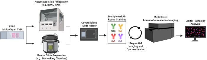
Figure 1: Schematic showing full multiplex immunofluorescence workflow. Please click here to view a larger version of this figure.

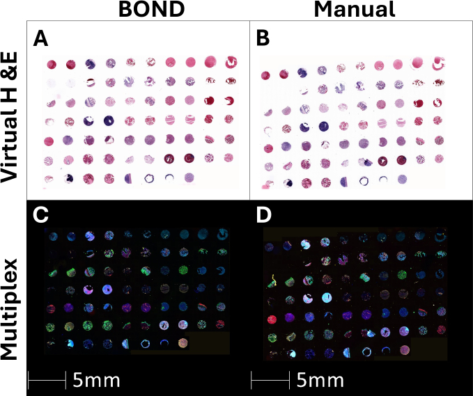
Figure 2: Overview of multiplex imaging: (A-B): Virtual H&E images generated from the DAPI staining and Cy3 autofluorescence of round 1 in order to visualise tissue integrity of the slides prepared using the automated slide stainer or manual slide preparation processes. (C-D): Multiplex IF staining of all biomarkers. Please click here to view a larger version of this figure.

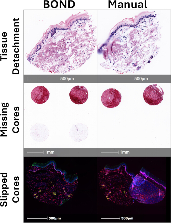
Figure 3: Examples of artefact types: Representative examples of different types of artefacts that can be generated primarily during slide preparation. Partial tissue detachment can be observed as out of focus regions and can cause issues with tissue alignment in subsequent rounds. Missing cores reduce experimental power and often happen disproportionately in delicate tissue types. Slipped or overlapping cores happen when a core detaches from its position on the TMA but clings to another region, compounding the loss of sample by making the hidden core difficult to analyse. Please click here to view a larger version of this figure.

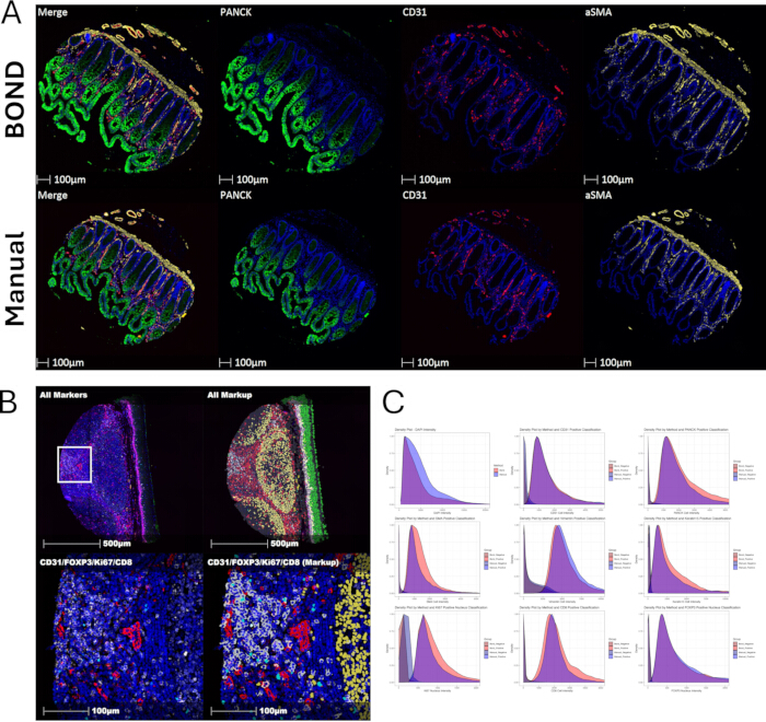
Figure 4: Comparison of BOND autostainer and manual slide preparation fluorescence signal: (A): Representative IF staining for structural markers pan cytokeratin (PANCK), CD31, and alpha smooth muscle actin (aSMA). A merge of these three images is shown in the first column. (B): Digital Pathology Software binary classification analysis masks, indicating positive marker detection across different cell type: CD31 (red), FOXP3 (turquoise), Ki67 (yellow), CD8 (white), PANCK (green). White box indicates digital zoom region in lower panels. (C): Quantitation of biomarker intensity in cell populations grouped by tissue preparation method (an automated slide stainer = red, Manual = blue) and marker positivity (dark = negative, light = positive). The area under each density plot represents 100% of the analyzed cell population. AF = Autofluorescence. Please click here to view a larger version of this figure.

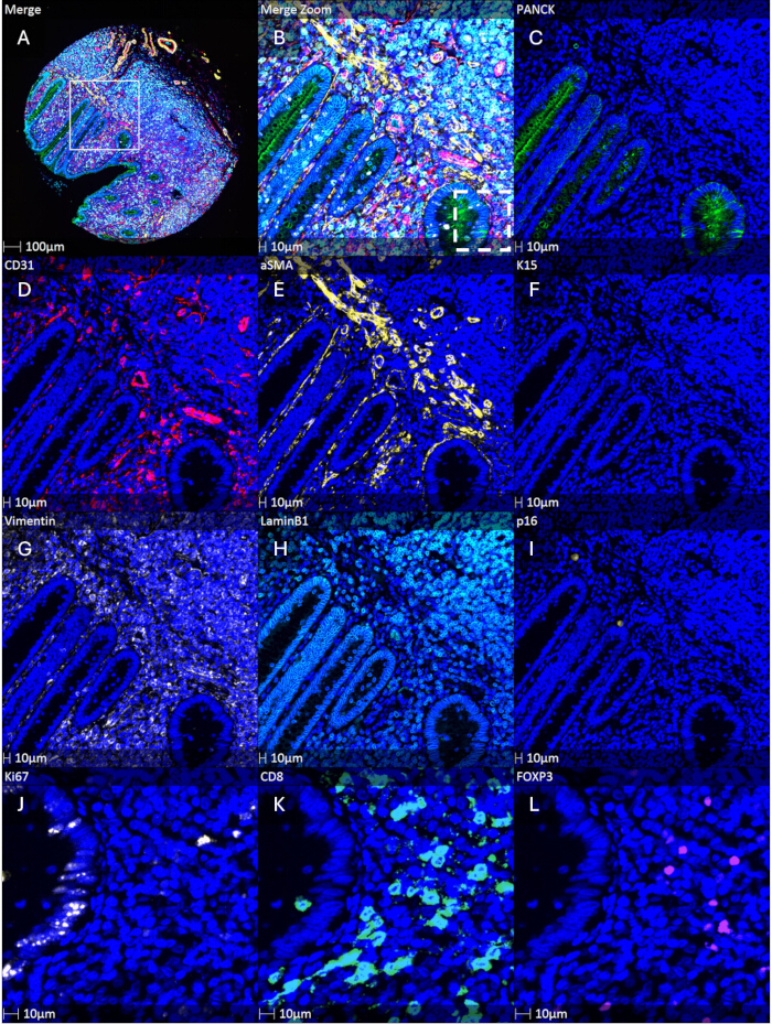
Figure 5: Full multiplex panel: Representative images from appendix tissue showing A-B: full 10-plex IF panel C: PANCK (green), D: CD31 (red), E:aSMA (yellow), F: K15 (pink), G: Vimentin (white), H: Lamin B1 (turquoise), I:p16 (gold), J: Ki67 (bright yellow), K: CD8 (bright green) and L: FOXP3 (purple). White box = digital zoom (Merge, CD31, aSMA, K15, Vim, LB1, p16), dashed box = digital zoom (Ki67, CD8, FOXP3). Please click here to view a larger version of this figure.

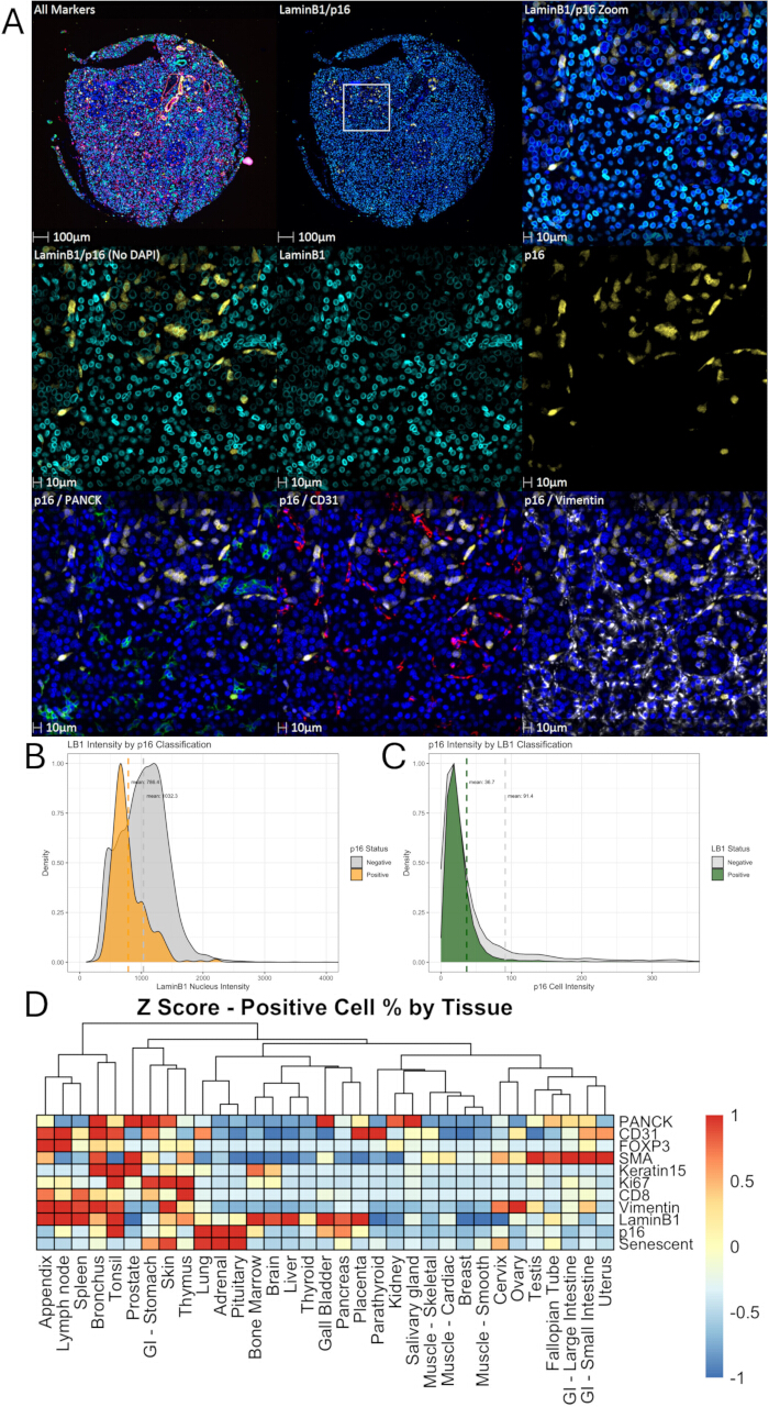
Figure 6: Senescence marker detection: (A): Representative IF from pancreas tissue images showing contrasting staining patterns of Lamin B1 (turquoise) and p16 (gold) along with spatial relationship to other markers PANCK (green), CD31 (red) and Vimentin (white). (B): Quantitation of Lamin B1 (LB1) nucleus intensity in p16 positive and negative cell populations. (C): Quantitation of p16 cellular intensity in Lamin B1 (LB1) positive and negative cell populations. Density plot area under curve represents 100% of the population. (D): Z-score normalized heatmap of average core percentage positivity for each biomarker or senescence phenotype (p16+/LB1-ve) across tissue types. Please click here to view a larger version of this figure.

Discussion

Multiplexed IF imaging through automated platforms facilitates the generation of nuanced profiles of a large panel of biomarkers within single tissue sections¹³. When paired with digital pathology software, such as HALO, this allows interrogation of both the abundance and spatial relationships of cell types, relative to one another as well as their distribution through different tissue structures³. This has the potential to bring significant value to the field of senescence, which relies on profiling combinations of hallmarks for robust classification of senescent cells, which in turn are established to possess significant heterogeneity and thus require single target cell profiling not possible with sequential tissue sections¹⁴. Furthermore, senescent cell burden varies across tissues, may accumulate at different rates during ageing, and there is an established paucity of reliable in vivo markers of senescence, making the ability to utilise a larger panel of biomarkers desirable in novel contexts where greater flexibility may be required^5,15,16. Importantly, previous studies have demonstrated that the accumulation and temporal dynamics of senescent cells are highly tissue-dependent, with substantial variation in both abundance and onset across organ systems, highlighting that senescence does not occur synchronously across tissues. Alternative spatial profiling techniques, such as spatial transcriptomics or imaging mass cytometry, can provide complementary molecular information; however, multiplex immunofluorescence directly measures protein expression and enables high-resolution spatial analysis of cell phenotypes within intact tissue sections. The sequential nature of multiplex IF also lends itself to an iterative discovery pipeline.

Multiplex IF imaging can be performed in high-throughput workflows by integrating with an automated slide stainer. In addition to providing significant advantages in terms of standardisation, the automated slide preparation also appears to lead to fewer artefacts than using a manual, decloaking chamber-based approach, as less tissue detachment and lost cores were observed. However, these observations are based on qualitative comparison, and further quantitative evaluation would be required to formally establish differences in processing-induced tissue damage. This is a particular concern in fatty tissue types such as skin and breast. Furthermore, the Coverslipless Slide Holder system allows integration with robotic plate handlers, enabling higher throughput and reducing operator time by facilitating workflow improvements such as overnight imaging runs. While automation is expected to improve throughput and standardisation, quantitative benchmarking of these improvements was not formally assessed in this study and should be interpreted as a practical observation rather than a measured outcome. With samples prepared as tissue microarrays, it becomes feasible to generate these comprehensive analyses for hundreds of patient samples across a relatively low number of slides which may facilitate future studies investigating senescent cells in clinical tissue samples^5,11.

Whilst slight increases in marker intensities using the automated slide stainer over the manual slide preparation process were observed, in practice this advantage is minor, as low signal can usually be overcome through either the use of longer exposure times or adjustments to analysis thresholds. Several key steps critically influence assay success, including antibody optimisation, multiplex panel design, and selection of imaging parameters. Careful validation of antibody compatibility, signal intensity, and resistance to repeated staining cycles is essential to ensure reproducible and high-quality multiplex data. Much more important is the round optimization and channel selection of biomarkers. These are assessed on test samples individually and in combination, to ensure the lack of cross-reactivity between antibodies, as well as to demonstrate that dye inactivation and epitope detection is possible in the desired rounds. It is recommended to use weak or less abundant markers in the Cy5 and Cy7 channels which typically exhibit lower autofluorescence. The final panel is tested in the tissue type of interest, as some widely used optimisation tissues (e.g. tonsil) often require lower concentrations and exposure times than experimental settings, which may also differ in properties such as autofluorescence. However, such positive control tissues can be useful when cell type presence is uncertain in experimental tissues, as lack of signal cannot be readily differentiated from the absence of target cells. Diligence in these panel optimisations within the target tissue type is the single most critical experimental step to ensuring a successful assay, to minimise the loss of biomarkers from final experimental runs. The majority of issues arise due to cross reaction of antibodies, insufficient signal due to low antibody concentrations or low signal to noise in FITC/Cy3 channels. Additionally, antigen preservation under repeated dye inactivation steps is both antibody and tissue-dependent, further necessitating the use of comprehensive optimisation steps to ensure selection of appropriate panel/round compositions for the experimental samples. A key limitation of multiplex immunofluorescence workflows is the dependence on high quality antibodies, together with the stability of epitopes across repeated staining and dye inactivation cycles.

Overall, the multiplexed imaging, coupled to automation platforms, represents a step-change in sophistication for the IF assessment of in vivo tissue samples, facilitating comprehensive spatial analysis of complex panels of biomarkers at the single-cell level. Future applications of this workflow include large-scale profiling of senescence-associated biomarkers across diverse tissue types and integration with emerging spatial omics approaches to further resolve cellular heterogeneity within complex tissue environments.

Materials

List of materials used in this article

Name	Company	Catalog Number	Comments
30% Hydrogen Peroxide (H2O2)	Merck	H1009
Antigen unmasking solution 1 (H3300) (ARS1)	Vector Labs.	H-3300	Prepare with 12.5 ml Antigen Unmasking Solution + 237.5 ml ddH2O
Antigen unmasking solution 2 (ARS2)	Sigma	T6066 / E5134	Prepare 10x stock (12.9 g Trizma base, 3.7 g EDTA, 5 mL Tween 20, 995 mL ddH20).
Bovine Serum Albumin (BSA)	Merck	A2153
Bulk Dewaxing Solution	Leica	AR9222
Bulk Epitope Retrieval 1 (ER1)	Leica	AR9961
Bulk  Epitope Retrieval (ER2)	Leica	AR9640
Bulk Wash Solution	Leica	AR9590
DAPI	Merck	D3571
Doubled distilled water (ddH20)	N/A	N/A
DMSO	Merck	472301
Donkey Serum	Merck	D9663
EDTA	Merck	E5134
Glycerol	Merck	G5516
NaHCO3	Merck	S5761
Phosphate Buffered Saline (PBS)	Merck	BP399
Propyl Gallate	Merck	P3130
Sodium Bicarbonate	Merck	S5761
Triton X 100	Merck	H5141
Trizma Base	Merck	T6066
Tween20	Merck	P1379
Other consumables or Equipment
Decloaking chamber	BioCare	DC2012
Steam strips	BioCare	613QC
Bond RXm Auto Slide Stainer	Leica	HIS2330	Referred to as automated slide stainer
Cell DIVE	Leica	29429159	Referred to as multiplex fluorescence imaging system
Click Well slide holders	Leica	29463259	Referred to as Well Coverslipless Slide Holder
Antibody List
CD31 (Pecam-1)	Cell Signalling	61255	Clone: 89C2 Fluorophore: AF555 Dilution: 1 in 50
CD8a	BioLegend	372906	Clone: C8/144B Fluorophore: Alexa 647 Dilution: 1 in 100
CDKN2A/p16	Santa Cruz	sc-56330 AF647	Clone: jc8 Fluorophore: Alexa 647 Dilution: 1 in 200
FOXP3	BioLegend	320114	Clone: 206D Fluorophore: Alexa 647 Dilution: 1 in 50
Keratin 15	Abcam	ab194065	Clone: EPR1614Y Fluorophore: AF_488 Dilution: 1 in 200
Ki67	Abcam	ab215226	Clone: EPR3610 Fluorophore: AF555 Dilution: 1 in 50
Lamin B1	Abcam	ab194106	Clone: EPR8985(B) Fluorophore: AF_488 Dilution: 1 in 100
PanCK_AE1/AE3	Thermofisher	53-9003-82	Clone: AE1/AE3 Fluorophore: AF_488 Dilution: 1 in 100
SMA	R&D systems	IC1420S	Clone: 1A4 Fluorophore: Alexa 750 Dilution: 1 in 100
Vimentin	Cell Signalling	69227	Clone: D21H3 Fluorophore: Alexa 750 Dilution: 1 in 100

References

- Gorgoulis, V., et al. Cellular senescence: Defining a Path Forward. Cell. 179 (4), 813-827 (2019).
- Hernandez-Segura, A., Nehme, J., Demaria, M. Hallmarks of cellular senescence. Trends Cell Biol. 28 (6), 436-453 (2018).
- De Souza, N., Zhao, S., Bodenmiller, B. Multiplex protein imaging in tumour biology. Nat Rev Cancer. 24 (3), 171-191 (2024).
- Teo, Y. V., et al. Notch signaling mediates secondary senescence. Cell Rep. 27 (3), 997-1007 (2019).
- Ogrodnik, M., et al. Guidelines for minimal information on cellular senescence experimentation in vivo. Cell. 187 (16), 4150-4175 (2024).
- Sharpless, N. E., Sherr, C. J. Forging a signature of in vivo senescence. Nat Rev Cancer. 15 (7), 397-408 (2015).
- Schürch, C. M., et al. Coordinated cellular neighborhoods orchestrate antitumoral immunity at the colorectal cancer invasive front. Cell. 182 (5), 1341-1359.e19 (2020).
- Lin, J. R., et al. Highly multiplexed immunofluorescence imaging of human tissues and tumors using t-CyCIF and conventional optical microscopes. eLife. 7, e31657(2018).
- Tomimatsu, K., et al. Precise immunofluorescence cancelling for highly multiplexed imaging to capture specific cell states. Nat Commun. 15, 3657(2024).
- Kiessling, P., Kuppe, C. Spatial multi-omics: novel tools to study the complexity of cardiovascular diseases. Genome Med. 16 (1), 14(2024).
- Chaib, S., Tchkonia, T., Kirkland, J. L. Cellular senescence and senolytics: the path to the clinic. Nat Med. 28, 1556(2022).
- Freund, A., Laberge, R. M., Demaria, M., Campisi, J. Lamin B1 loss is a senescence-associated biomarker. Mol Biol Cell. 23 (11), 2066-2075 (2012).
- Eng, J., et al. A framework for multiplex imaging optimization and reproducible analysis. Commun Biol. 5 (1), 1-11 (2022).
- Wallis, R., et al. Senescence-associated morphological profiles (SAMPs): an image-based phenotypic profiling method for evaluating inter- and intra-model heterogeneity of senescence. Aging (Albany NY). 14, 1-27 (2022).
- González-Gualda, E., Baker, A. G., Fruk, L., Muñoz-Espín, D. A guide to assessing cellular senescence in vitro and in vivo. FEBS J. 288 (1), 56-80 (2021).
- O’Sullivan, E. A., Wallis, R., Mossa, F., Bishop, C. L. The paradox of senescent-marker positive cancer cells: challenges and opportunities. NPJ Aging. 10 (1), 1-11 (2024).
Reprints and Permissions