An Integrated Multimethod Simulation Framework for Tin Debris Control in Extreme Ultraviolet Lithography

Summary

This protocol aims to guide users through an integrated simulation framework to achieve tin debris control in extreme ultraviolet (EUV) and emerging Blue-X lithography, integrating kinetic modeling, the Boltzmann transport equation (BTE), and density functional theory (DFT)–based methods to evaluate ion interactions and hydrogen-assisted cleaning.

Abstract

This protocol is a conceptual, integrated modeling framework illustrated with representative results and instructs users on combining the Boltzmann transport equation (BTE), particle-in-cell (PIC), and kinetic simulations to investigate tin (Sn) debris mitigation in extreme ultraviolet (EUV) lithography. The protocol includes the reflectivity of Mo/Si multilayer mirrors (MLM), sputtering yield, implantation depth, kinetic modeling, and BTE computation. BTE and PIC simulations are used to resolve the electron energy distribution function (EEDF) of hydrogen plasmas and analyze the generation and acceleration of energetic Sn ions under different plasma conditions. The influence of hydrogen flow on ion slowing and radiation efficiency is also quantified. Based on the ionization cross sections and dissociation channels of Sn_xH_y species, the interaction potentials for Sn-H collision are computed using the density functional theory (DFT) method, which are used to calculate the implantation depth. In addition, the MLM reflectivity and sputtering yield from the interaction between Sn debris and the Ru coating on the MLM are calculated using a semi-empirical formula. By following this protocol, users can obtain key physical parameters relevant to Sn debris control, including sputtering yields, implantation depths, MLM reflectivity, and SH₄ formation under various hydrogen plasma EEDFs. These outputs enable systematic evaluation of contamination, cleaning, and detection processes in EUV lithography systems.

Introduction

Extreme-ultraviolet lithography (EUVL) is the state-of-the-art technology for advancing integrated circuit miniaturization, enabling patterning of features smaller than 2 nm. In a typical EUV source, a tin (Sn) microdroplet is first vaporized and ionized by a prepulse from a Nd:YAG laser, and the resulting plasma cloud is reheated by a CO₂ laser operating at 10.6 µm, thereby generating EUV radiation, which is collected by Mo/Si multilayer mirrors (MLM)^1,2. For commercial systems such as those developed by ASML, source power has reached levels sufficient for mass production. Nevertheless, ongoing research—particularly in China—continues to focus on improving the efficiency of CO₂ laser-produced Sn plasmas.

One major challenge in EUV light sources is the production of energetic Sn ions. Irradiation of Sn droplets with high-intensity CO₂ laser pulses generates ions with energies in the keV range, which can damage multilayer mirrors (MLMs) and shorten system lifetime^3,4,5. To reduce ion-induced damage, hydrogen (H₂) is widely employed as a buffer gas. By collisional slowing, H₂ mitigates Sn ion transport and reduces debris reaching optical components. Reliable stopping power data and accurate models of Sn–H interactions are therefore crucial for optimizing both source efficiency and durability^5,6,7.

Another important issue is linked to the deposition of Sn fragments on surfaces within the vacuum chamber, particularly the collector mirrors positioned near the plasma. Even a thin Sn coating reduces EUV reflectivity and degrades optical performance and operational stability^8,9,10. A practical industrial solution is the continuous injection of H₂ as a background gas¹¹. In this approach, hydrogen radicals etch Sn coatings through the following exothermic reaction, producing volatile stannane (SnH₄), which is removed by pumping.

Sn(s) + 4H(g) → SnH₄(g),

While effective in enhancing Sn removal, this method introduces new complications. Hydrogen radicals produced from H₂ plasma dissociation can induce chain decomposition of SnH₄, regenerating Sn and causing secondary contamination⁹. Such processes reduce cleaning efficiency and may compromise mirror stability and optical performance. A detailed understanding of tin hydride formation, decomposition, and surface interactions is thus essential for improving hydrogen-based cleaning methods. Recent surface studies underscore the importance of characterizing tin hydrides and their intermediates to correctly identify contamination pathways and suppress Sn redeposition¹².

Despite these efforts, key aspects of Sn–H plasma chemistry remain insufficiently characterized. In particular, the structure, reactivity, fragmentations, and formation/dissociation rates of Sn-H species (e.g., Sn₂H₂ and SnH_x) under EUV-relevant plasma conditions lack direct experimental validation¹³. Furthermore, side reaction pathways in Sn-H plasmas, the factors governing their occurrence probabilities, critical thresholds for adverse reactions, and long-term operational stability have not been systematically investigated¹⁴.

Taken together, these issues underscore the need for fundamental investigations of plasma–surface interactions from the perspectives of atomic and molecular physics, plasma physics, and quantum chemistry. Existing modeling approaches typically address only isolated aspects of the Sn debris control, such as Sn ions generation, stopping power of H₂ to high-energy Sn ions, or ion-surface interaction, and therefore, cannot capture the full contamination–cleaning–detection cycle. To address these limitations, we aimed to develop an integrated simulation protocol that combines particle-in-cell (PIC) simulations, Boltzmann transport equation (BTE) analysis, density functional theory (DFT), and kinetic modeling. Extreme ultraviolet (EUV) light source studies involve multiple coupled processes, including laser–droplet, laser–plasma, plasma–plasma, and plasma–gas interactions. This protocol describes an integrated simulation framework combining fluid dynamics, particle-in-cell (PIC), and density functional theory (DFT) methods to model tin (Sn) debris mitigation and hydrogen cleaning. This protocol provides a unified, reproducible workflow for investigating Sn debris generation, transport, surface interactions, and hydrogen-assisted mitigation. The following section details the step-by-step implementation of this methodology.

Protocol

NOTE: The overall workflow, including the integration of fluid, kinetic, and quantum-chemical approaches. The workflow is illustrated in Figure 1 (highlighted in the red box).

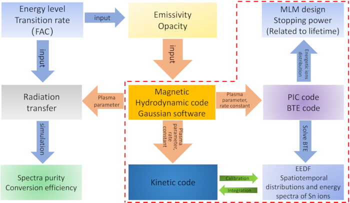
Figure 1. Schematic of the integrated simulation framework for extreme ultraviolet lithography. Abbreviations: MLM = multilayer mirrors; PIC = particle-in-cell; BTE = Boltzmann transport equation; EEDF = Electron energy distribution function. Please click here to view a larger version of this figure.

1. MLM reflectivity simulation

1. Set up multilayer parameters. Use Mo/Si MLMs as collectors in EUV sources. Define Mo/Si multilayer mirror (MLM) structure with the following layer thicknesses: Mo (1.950 nm), Mo-on-Si (0.806 nm), Si (3.843 nm), and Si-on-Mo (0.386 nm)¹⁵.
2. Evaluate surface protection materials. As the Mo/Si surface is prone to oxidation and carbide formation, which reduces optical performance over time, include Ru, RuO₂, ZrO₂, and TiO₂ coatings to assess oxidation and carbide resistance¹⁶.
3. Calculate MLM reflectivity. Evaluate the reflectivity of a Mo/Si multilayer with a Ru capping layer using refractive index data, enabling a quantitative assessment of trade-offs between protection and optical efficiency.
   
   
   
   NOTE: δ and β values for different materials are available at the Center for X-Ray Optics at Lawrence Berkeley National Laboratory¹⁷.
4. MLM reflectivity against Ru capping layer: Compute reflectivity changes as a function of capping-layer thickness using refractive indices. Compare results to determine the trade-off between optical efficiency and durability (Figure 2).
5. Output and reproducibility checkpoint: Confirm successful execution of this section by generating a reflectivity–thickness curve at 13.5 nm as Figure 2 or the reference values reported by Liu et al.¹⁵.

Figure 2. Reflectivity of a Mo/Si multilayer with varying thicknesses of the Ru capping layer. Please click here to view a larger version of this figure.

2. Sputtering yield calculation

1. Apply the Yamamura formula. Calculate the sputtering yield (Y) using the formula proposed by Yamamura et al.¹⁸
2. Compute stopping cross sections. Evaluate nuclear (S_n) and electronic (S_e​) stopping cross sections using Eqs. (3)–(4).
   
   and
3. Determine constants. Calculate the empirical constant K using Eq. (5)
   
   Where Z₁ and Z2 represent the atomic number of the incident projectile and target material, respectively; m1 and m2 represent the mass of the incident projectile and target material, respectively. E_r and E_th are the reduced energy and threshold energy, respectively, E_s is the surface binding energy of target material¹⁸.
4. Execution steps: Calculate the sputtering yield by executing the Python script shown in Figure 3. Implement the Yamamura formula using the Python script shown in Figure 4. Ensure that the computer is equipped with Python 3 and the NumPy library. Executing the Python script shown in Figure 3 generates a two-column text file named yield.dat containing the calculated sputtering yields, as shown in Figure 5.
5. Reproducibility checkpoint: Confirm successful execution of this section by generating a sputtering-yield–versus–incident-energy curve for Sn ions impacting Ru (Figure 5). Verify that the calculated sputtering yield for Ar on Ru agrees with published experimental data within ±30%, serving as a calibration check.

Figure 3. Python script for calculating sputtering yield. Please click here to view a larger version of this figure.

Figure 4. Python script for Yamamura formula. Please click here to view a larger version of this figure.

Figure 5. Calculated sputtering yields of Ar in Ru and Sn in Ru. Left: Ru; right: Sn in Ru. Yamamura et al.’s formula described in Step 2.1 was used. The comparison between present simulations and those of Wu et al.²⁶ and Laegreid et al.²⁷ are performed. Please click here to view a larger version of this figure.

3. Implantation depth simulation

1. Select the potential model. Use the KrC potential in the RustBCA code¹⁹ for ion–solid interactions:
2. Define screening function. Implement Φ(r/a) as a sum of exponential terms:
   
   1. Express the value of a for KrC potential as in the following equation with other parameter c_i and d_i from Table 1.
3. Execution steps: Calculate the implantation depth by executing the Python script shown in Figure 6, where the RustBCA execution command is integrated into the script:
   1. Type the command = "cargo run --release 1D "+ InputFile
   2. Then, type os.system(command)
4. Open the Python script shown in Figure 6, set the parameters according to the script, and run it to obtain a two-column text file named depth.dat, which contains the calculated implantation depth.
5. Reproducibility checkpoint: Confirm successful execution of this section by generating an average implantation depth of Sn (Figure 7).

c1	c2	c3	d1	d2	d3
0.19095	0.47367	0.33538	0.27854	0.63717	1.91925

Table 1: The parameter c_i and d_i involved in KrC potential.

Figure 6. Python script for calculating implantation depth. Please click here to view a larger version of this figure.

Figure 7. Calculated implantation depth of Sn ions in Ru-Mo-Si multilayer mirrors. Left: The implantation depth distribution of 10000 incident Sn ions at two incident energy, 2.0 keV (yellow) and 3.0 keV (blue); Right: The average implantation depth of Sn. Calculated by KrC potential implemented in RustBCA described by protocol step 3.1. Please click here to view a larger version of this figure.

4. Stopping power calculation

1. Model hydrogen as a buffer gas. To mitigate the damage of keV Sn ions to MLM, introduce hydrogen as a buffer gas.
   NOTE: Hence, the stopping power and sputtering of keV Sn ions in the presence of hydrogen and MLM surfaces remain critical issues.
2. Use DFT-based potentials. Fit the calculated interatomic potentials for hydrogen–metal systems to both the Ziegler–Biersack–Littmark (ZBL) and Morse potential forms.
   NOTE: In a recent work²⁰, an interatomic potential for hydrogen–metal systems based on density functional theory (DFT) calculations has been developed.
3. Reproducibility checkpoint: Validate the computed stopping power of Sn ions in hydrogen by comparing the energy-dependent stopping curves with reference data obtained from SRIM simulations and published experimental datasets.
   NOTE: These data should be compared to Figure 6 of Feng et al.²⁰.
4. Combine outputs from Sections 1–4 (MLM reflectivity, sputtering yield, implantation depth, and stopping power) to estimate the relative lifetime of Mo/Si multilayer mirrors under Sn ion exposure.
   NOTE: Effects such as surface roughness evolution, mirror geometry, and ray tracing are not included in the present protocol and should be incorporated in future extensions.
5. Apply the same workflow to alternative wavelength regimes, such as Blue-X lithography, by adjusting optical constants and ion energy distributions accordingly.

5. SnH₄ formation and decomposition

NOTE: Detailed kinetic study of formation and decomposition of SnH₄ requires several cross sections and reaction rates between Sn-H. Previously, some electron-impact ionization and fragmentation of stannane²¹, reaction rates of XH₄+H→XH₃+H₂ and SnH₄+SnH→Sn₂H₃+H₂, SnH₄+SnH→Sn₂H₅^22,23 have been reported. However, the plasma-phase formation of SnH₄, as well as the interactions and reaction mechanisms with various materials, have not yet been fully characterized or understood. Experimental studies on stannane chemistry and related decomposition pathways, therefore, remain scarce^12,24, highlighting the need for further investigation.

1. DFT and TST calculations: Use density functional theory (DFT) in combination with transition state theory (TST) implemented in Gaussian 16 to calculate missed reaction rates.
   NOTE: These computational approaches allow for the calculation of reaction energetics, transition states, and rate constants, providing a detailed mechanistic understanding of stannane formation under plasma conditions.
2. Define reaction pathways. Two successive reaction pathways leading to the formation of SnH₄ are included here.
   (1) Sn+H₂→SnH₂
   (2) SnH₂+H₂→SnH₄
3. Perform DFT and TST calculations. Calculate reaction energies, transition states, and rate constants (k) for the two reactions, with the results shown in Figure 8 and Figure 9. Summarize reaction thermodynamics in Table 2 and Table 4 and Arrhenius parameters in Table 3 and Table 5.
4. Output and reproducibility checkpoint: Validate the computed reaction rate constants by reproducing the temperature-dependent rate curves shown in Figure 8 and Figure 9, or with reported values^22,23.
5. Export the validated rate constants in tabulated or machine-readable format (e.g., CSV or TXT) for direct use as input parameters in subsequent kinetic modeling of Sn–H plasma chemistry.

Figure 8. The reaction rate and energy barrier for Sn+H₂→SnH₂. Left: Reaction rate constants of Sn+H₂→SnH₂; Right: energy barrier for the reaction pathways (All gray atoms represent H, and blue atoms represent Sn). The calculations are performed by Gaussian 16. Please click here to view a larger version of this figure.

Reaction	Product	ΔH	ΔG	ΔE
Sn+H2→SnH2	SnH2	-24.71	-19.13	17.87

Table 2: Reaction Enthalpies (H), Gibbs free energy (G) and potential barriers (E) (kcal/mol) for the three reaction channels at 298.15 K and 1 atm.

Arrhenius Parameters	Methods	Reactions
		Sn+H2→SnH2
A	TST	2.50×10-13
	TST/Wigner	1.13×10-13
	TST/Eckart	1.45×10-29
n	TST	0.85
	TST/Wigner	0.93
	TST/Eckart	5.56
Ea(kJ/mol)	TST	68.99
	TST/Wigner	65.3
	TST/Eckart	30.4
k(298K)(cm3mol-1sec-1)	TST	2.72×10-23
	TST/Wigner	8.94×10-23
	TST/Eckart	1.03×10-21

Table 3: Arrhenius parameters of Sn+H₂→SnH₂ reaction within the temperature range of 180 to 2000 K.

Figure 9. The reaction rate and energy barrier for SnH₂+H₂→SnH₄. Left: Reaction rate constants of SnH₂+H₂→SnH₄; Right: energy barrier for the reaction pathways (All gray atoms represent H, and blue atoms represent Sn). The calculations are performed by Gaussian 16. Please click here to view a larger version of this figure.

Reaction	Product	ΔH	ΔG	ΔE
SnH2+H2→SnH4	SnH4	-26.5	-32.81	26.26

Table 4: Reaction Enthalpies (H), Gibbs free energy (G) and potential barriers (E) (kcal/mol) for the three reaction channels at 298.15 K and 1 atm.

Arrhenius Parameters	Methods	Reactions
		SnH2+H2→SnH4
A	TST	3.73×10-17
	TST/Wigner	1.23×10-17
	TST/Eckart	1.29×10-37
n	TST	1.55
	TST/Wigner	1.67
	TST/Eckart	7.5
Ea(kJ/mol)	TST	136.39
	TST/Wigner	132.94
	TST/Eckart	90.83
k(298K)(cm3mol-1sec-1)	TST	3.39×10-37
	TST/Wigner	9.33×10-37
	TST/Eckart	6.56×10-36

Table 5: Arrhenius parameters of SnH₂+H₂→SnH₄ reaction within the temperature range of 180 to 2,000 K.

6. Electron energy distribution function (EEDF) calculation

NOTE: Boltzmann transport equation

The Boltzmann equation for an ensemble of electrons in an ionized gas is

Where f is the electron distribution in six-dimensional phase space, v are the velocity coordinates, e is the elementary charge, m is the electron mass (9.10956 × 10^-31 kg), E is the electric field,  is the velocity-gradient operator, and C represents the rate of change in f due to collisions.

1. Run BOLSIG+ solver using the two-term approximation to solve the Boltzmann transport equation for hydrogen plasma²⁵.
2. Execution steps: BOLSIG+ is a graphical window.
   1. Click the Read collisions button as shown in Figure 10A to read the cross sections data of H₂.
   2. Select the calculation parameters in the “conditions” file as shown in Figure 10B.
   3. Finally, as presented in Figure 10C, click the plot EEDF button to draw the EEDF image.
3. Output and reproducibility checkpoint: Confirm successful execution of the BOLSIG+ solver by generating the electron energy distribution function (EEDF) for hydrogen plasma over the specified reduced electric field (E/N) range. Verify that the EEDF with Figure 11.
4. Export the final EEDF data in tabulated form (e.g., ASCII or CSV format) for direct use as input in kinetic modeling of Sn–H plasma chemistry.

Figure 10. The graphical interface of BOLSIG+ software. Please click here to view a larger version of this figure.

7. Kinetic modeling of Sn–H plasma chemistry

1. Import plasma parameters from PIC simulations. Extract plasma parameters, including electron density and plasma temperature, from fluid simulations. Use these parameters as initial conditions for PIC simulations to obtain the spatiotemporal distributions and energy spectra of Sn ions.
2. Perform kinetic simulations. Solve the coupled rate equations for Sn, SnH_x, and related intermediates using the PIC-derived ion energy distributions and DFT/TST-derived reaction rates as inputs. Track the temporal evolution of species densities under hydrogen plasma conditions relevant to EUV source operation.
3. Couple kinetic outputs with surface interaction models. Combine kinetic results with stopping power, sputtering yield, and implantation depth distributions obtained in sections 2–4. Use these coupled outputs to evaluate degradation mechanisms and estimate the effective lifetime of Mo/Si MLM.

Results

Sputtering yield calibration and validation
Calculate the sputtering yield of Ar atoms in Ru as a calibration step. These sputtering yields represent output from protocol step 2.1 (Yamamura model). The results are shown in Figure 5 (left). Experimental data reported by Wu et al.²⁶ and Laegreid et al.²⁷ are largely consistent. The theoretical results from the present model show good agreement with experimental measurements a...

Discussion

The integrated methodology that combines the Boltzmann transport equation (BTE), particle-in-cell (PIC), and kinetic simulations establishes a unified framework for investigating tin (Sn) debris mitigation in extreme ultraviolet (EUV) lithography. Specifically, the fluid simulation yields the plasma parameters—density and temperature, which can be integrated into a PIC program to obtain the spatiotemporal distribution of Sn_xH_y molecules. By coupling these PIC results with reaction rates obtain...

Materials

List of materials used in this article

Name	Company	Catalog Number	Comments
BOLSIG+	Laboratory Plasma et Conversion d'Energie, University Paul Sabatier	The version updated on April 24, 2025
Gaussian	Gaussian Inc.	Gaussian 16
RustBCA	Department of Nuclear, Plasma, and Radiological Engineering, University of Illinois at Urbana-Champaign	1.2.0