A Protocol For Uncovering Neural Mechanisms Of Neurotherapeutic Effects On Electroencephalography Using The Human Neocortical Neurosolver

Summary

This protocol demonstrates how physics-based neural simulations can be used to interpret electrophysiological biomarkers of neurotherapeutics and uncover their effect on neural circuits, providing a mechanistically grounded approach for neurotherapeutic development.

Abstract

Electroencephalography (EEG) and electrophysiological methods provide millisecond-resolution biomarkers for central nervous system disorders and are widely used to assess treatment-related effects. However, limited understanding of the neural mechanisms generating these biomarkers impedes the development of diagnostics and therapeutics based on these signals. The Human Neocortical Neurosolver (HNN) is an open-source biophysical modeling software that links localized EEG biomarkers to their multiscale neural generators. This protocol demonstrates a hypothesis-driven workflow using HNN to test neural mechanisms of neurotherapeutic-induced EEG biomarkers by optimizing model parameters to achieve a fit between simulated and empirical current source waveforms. Corresponding multiscale cell- and circuit-level activity can then be visualized and quantified, providing validation targets for model predictions in follow-up empirical studies. An example is provided demonstrating how to examine the neural mechanisms underlying early event-related potential components of an auditory evoked response (P1, N1, and P2), and to assess changes following neurotherapeutic-induced modifications in neural circuit activity. This protocol enables the design of simulation experiments to generate testable predictions linking EEG biomarkers to underlying neural circuit mechanisms. A similar workflow can be applied to study disease mechanisms or other therapeutic interventions.

Introduction

Central nervous system (CNS) therapeutic development faces unique challenges, with approval rates lower than in other disease areas, highlighting the need for innovative methodological approaches¹, particularly those that can uncover treatment-related effects on brain dynamics. A well-established approach to study the effect of therapeutics on neural activity is electroencephalography (EEG)^2,3. EEG provides a signature of in vivo circuit-level brain dynamics and offers strong translational potential from rodent models to human trials, as the neural circuitry generating EEG signals shows homology across species^4,5,6,7,8. In pharmaceutical development, EEG can serve multiple roles, including providing translational readouts between animal and human studies, evaluating drug safety, guiding compound selection, informing dose-response relationships, assessing proof-of-mechanism in early clinical phases, and enabling clinical trial stratification and cohort enrichment^{9,10,11,12,13,14}. Despite these advantages, the interpretation of EEG signals remains a major challenge, particularly when attempting to link observed changes to underlying neural mechanisms.

A robust EEG biomarker used in CNS drug discovery is the event-related potential (ERP). ERPs reflect time-locked sensory-evoked brain activity and have been widely used to study neurodevelopmental and neuropsychiatric disorders, including depression^15,16, schizophrenia^17,18, autism spectrum disorder^19,20, and Alzheimer’s disease²¹. ERPs are also used to assess treatment effects and dose ranges on brain circuits^22,23,24,25, where normalization toward healthy responses may indicate therapeutic efficacy²⁶. However, a key limitation of ERPs and other EEG biomarkers (e.g., brain oscillations) is that their associations with disease states or drug effects are largely correlational. While statistical analyses can identify relationships between biomarkers and outcomes, they do not provide mechanistic insight into how specific neural circuit elements generate these signals. The causal contributions of specific cell types and circuit mechanisms therefore remain unclear. Understanding the cellular and circuit origins of EEG signals could considerably enhance their value by linking observed signatures to underlying physiology^27,28. In this manuscript, the term EEG “biomarker” refers to measurable changes in EEG signals following therapeutic intervention, consistent with the Food and Drug Administration–National Institutes of Health Biomarkers, EndpointS, and other Tools (FDA–NIH BEST) framework definition²⁹, rather than implying formal qualification for a specific clinical use³⁰.

While invasive electrophysiological recordings can provide detailed cell- and circuit-level insights, these approaches are largely restricted to animal models and are difficult to translate directly to human studies. Alternative approaches, such as inverse modeling techniques, can estimate source activity from EEG signals but often lack explicit mechanistic representations of underlying neural circuitry. Biophysical simulations offer a complementary framework by modeling the physical processes through which neural circuits generate measurable EEG signals^31,32,33,34 (Figure 1). Compared to purely statistical biomarker analyses or inverse methods without mechanistic grounding, biophysical modeling enables direct testing of hypotheses linking neural circuit dynamics to observed electrophysiological signals.

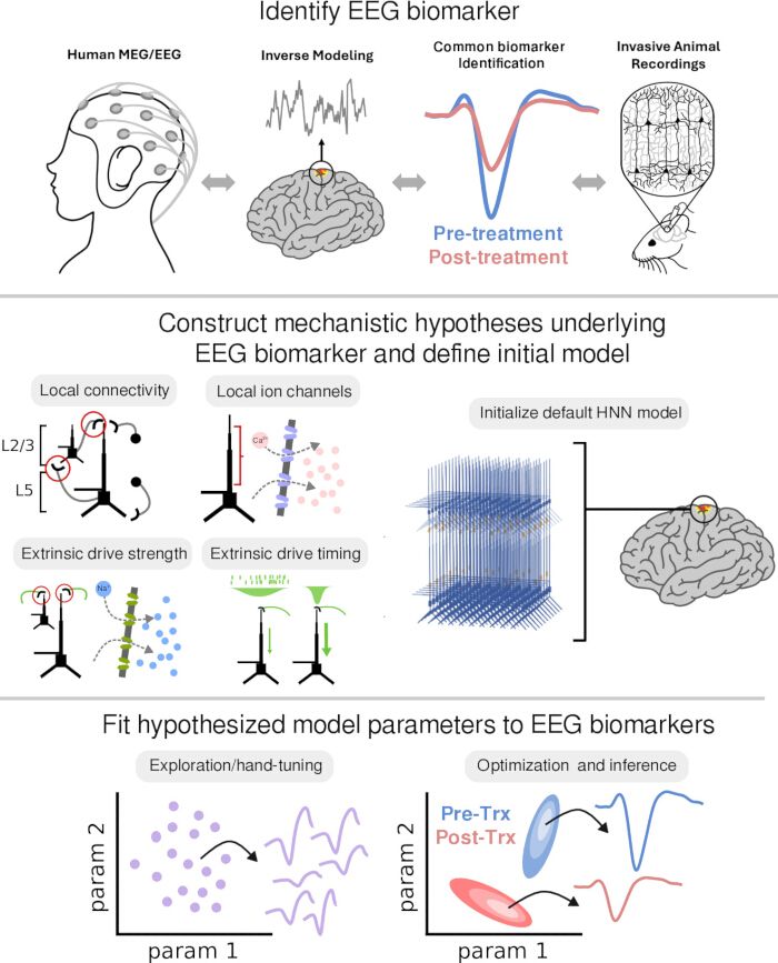
Figure 1. Biophysical modeling to develop and test mechanistic hypotheses underlying pharmacological electroencephalography (EEG) biomarkers. (A) Identification of an EEG biomarker based on differences in brain signals between conditions. An example is an auditory event-related potential (ERP) that is reduced in the post-treatment condition (red) relative to the pre-treatment condition (blue). (B) Biophysical modeling enables testing of mechanistic hypotheses explaining how EEG biomarkers arise and change with pharmacological intervention. Hypotheses are formulated regarding drug-induced changes in neural activity, and corresponding model parameters are identified. (C) The default Human Neocortical Neurosolver (HNN) model is used as a starting point to test hypotheses by manually modifying model parameters or applying automated optimization and inference algorithms. Differences in parameter values between pre-treatment and post-treatment conditions correspond to model-based predictions. Please click here to view a larger version of this figure.

This protocol uses the Human Neocortical Neurosolver (HNN), an open-source biophysical modeling framework, to link ERP biomarkers of treatment-related effects to their underlying cell- and circuit-level mechanisms³³ (Figure 2). HNN is based on the principle that synchronous intracellular current flow in aligned pyramidal neuron dendrites generates the primary current dipoles underlying EEG signals^6,35,36,37. The model represents a canonical neocortical column consisting of excitatory pyramidal neurons and inhibitory interneurons distributed across cortical layers 2/3 and 5. The default HNN network includes 100 pyramidal neurons and 33 inhibitory neurons per layer, forming a reduced yet biologically grounded representation of cortical circuitry. Pyramidal neurons are modeled with multicompartment dendritic structures to capture key morphological features³⁸, while inhibitory neurons are represented as single compartments due to their limited contribution to extracellular currents³³. Synaptic interactions include excitatory α-amino-3-hydroxy-5-methyl-4-isoxazolepropionic acid (AMPA) and N-methyl-D-aspartate (NMDA) receptors, and inhibitory gamma-aminobutyric acid type A and gamma-aminobutyric acid type B (GABA_B) receptors, with all neurons incorporating active ionic conductances governed by Hodgkin–Huxley dynamics.

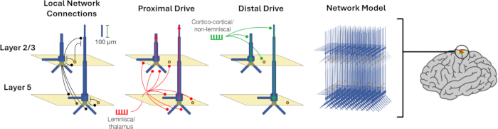
Figure 2. Schematic of the HNN model. Visualization of the major components of the HNN model, including local network connections between excitatory and inhibitory neurons, and exogenous input pathways termed “proximal drive” and “distal drive.” Please click here to view a larger version of this figure.

Neural activity in HNN is driven by exogenous inputs representing feedforward and feedback pathways. Feedforward “proximal” drives correspond to inputs from lemniscal thalamus which target proximal dendrites, while feedback “distal” drives represent cortico-cortical and non-lemniscal thalamic inputs targeting distal dendrites. These inputs are modeled as trains of action potentials that evoke synaptic currents and generate intracellular current flow along pyramidal neuron dendrites. The resulting population-level current dipole is expressed in nanoampere-meters, enabling direct comparison with orientation-constrained source-localized EEG or magnetoencephalography (MEG) data. The default parameterization of HNN is informed by empirical data from somatosensory cortex studies^39,40,41 and has been successfully applied to auditory^42,43,44, visual⁴⁵, and frontal cortical signals⁴⁶, with model-derived predictions validated in subsequent experimental studies^7,41,47.

HNN simulations can be applied at multiple stages of pharmaceutical research and development, including target validation, comparison of drug mechanisms of action, dose optimization, and hypothesis generation for follow-up experiments^14,48,49,50. This enables users to incorporate mechanistic modeling into practical research workflows, supporting the generation and testing of hypotheses about how neurotherapeutics influence neural circuits. In this protocol, we focus on the early P1, N1, and P2 components of auditory ERPs, as these features are well characterized and provide constraints for hypothesis-driven modeling⁵¹. While the focus is on drug-induced changes, the approach can be extended to other neurotherapeutic interventions, such as brain stimulation or behavioral training, as well as to studies of CNS disorders.

The use of HNN follows an iterative modeling framework in which model structure and parameters are initially constrained by existing data and then refined through comparison with empirical observations. Large-scale neural models contain many parameters, but only a subset—referred to as parameters of interest—are adjusted to test specific hypotheses. These parameters are not selected arbitrarily; rather, they are chosen based on prior experimental evidence and literature describing potential mechanisms of action of the neurotherapeutic. In this protocol, parameters related to exogenous input timing and strength, local inhibitory connectivity, and dendritic ion channel conductances are selected as examples of biologically interpretable variables that may be influenced by neurotherapeutics.

Beginning with a default model, users first fit parameters to pre-treatment ERP data using a combination of manual tuning and automated optimization. Manual tuning adjusts global scaling and input parameters to approximate the empirical waveform, providing an intuitive understanding of how parameter changes affect model output. Automated methods such as covariance matrix adaptation evolution strategy (CMA-ES), Bayesian optimization, and constrained optimization by linear approximation are then used to refine parameter values and improve the fit. Once a pre-treatment model is established, parameters hypothesized to account for post-treatment changes are adjusted to fit post-treatment ERP data.

To address uncertainty in parameter estimation, simulation-based inference (SBI) is used to estimate distributions of parameter values that reproduce the observed data^52,53. SBI accounts for the possibility that multiple parameter combinations can produce similar outputs and enables quantification of parameter uncertainty. Differences between pre-treatment and post-treatment parameter distributions can be assessed using an overlap index (OVL)^54,55, providing insight into potential mechanisms of action.

A key advantage of this approach is that fitting the model to a specific data modality generates predictions across multiple scales of neural activity, including cell spiking, layer-specific local field potentials (LFPs), and current source density (CSD). These predictions provide targets for experimental validation using complementary techniques. If predictions are not supported by empirical data, the model can be updated by incorporating new constraints, forming an iterative cycle of hypothesis generation, testing, and refinement (Figure 3).

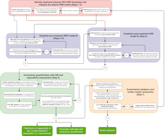
Figure 3. Iterative workflow for developing and testing ERP biomarker predictions with HNN. The workflow corresponds to the protocol steps. Identification of an EEG biomarker and initialization of the default HNN model are shown in red (Steps 1–2). Manual tuning and optimization are used to fit model parameters to pre-treatment and post-treatment ERP signals (purple; Steps 3–5). Uncertainty quantification using simulation-based inference (SBI) is shown in green (Step 6). Model predictions are then examined and compared with experimental data to validate or further constrain the model (orange; Step 7). Please click here to view a larger version of this figure.

This protocol is designed for use with orientation-constrained, source-localized EEG or MEG data collected during evoked response paradigms. Standard preprocessing and source localization methods (e.g., minimum norm estimation [MNE]-Python⁵⁶) can be used to generate the required input data. Source-level signals expressed in nanoampere-meters are directly comparable to HNN outputs. For fast sensory responses, source- and sensor-level signals are often highly similar, allowing insights from source-localized modeling to inform interpretation of sensor-level EEG data^57,58.

Protocol

All procedures involving human data were performed in accordance with relevant institutional guidelines and regulations. The dataset used in this study was obtained from a previously published study⁴³, and no additional ethical approval was required. No hazardous materials or procedures are involved in this protocol.

1. Identify a treatment-induced EEG event–related potential biomarker and define model hypotheses

1. Collect or identify a dataset containing experimentally recorded EEG signals from subjects of interest (e.g., pre-treatment and post-treatment in the context of neurotherapeutics). Record EEG measurements during presentation of a sensory stimulus and record timestamps of the sensory stimulus simultaneously with EEG data to enable segmentation into trials. Ensure that EEG data are stored in a format compatible with preprocessing software (e.g., .fif, .set, or .edf).
   NOTE: The associated code repository (https://github.com/ntolley/hnn_jove) provides the data files used to generate the representative results. The repository includes a preprocessed auditory MEG ERP from Kohl et al. (2022), which serves as the pre-treatment ERP (original data available at: https://github.com/kohl-carmen/HNN-AEF). The hypothetical post-treatment ERP is generated by scaling the pre-treatment waveform using a Gaussian-tapered window. The corresponding data files are located in the repository at data/pre-treatment.txt and data/post-treatment.txt. Because MEG and EEG signals reflect similar underlying neural generators, this protocol is applicable to both modalities.
2. Identify a set of candidate ERP biomarker features that are hypothesized to distinguish treatment-related effects (e.g., ERP peak timings and magnitudes).
   NOTE: In this example protocol, peak magnitudes are used as a biomarker of interest.
3. Preprocess EEG data and extract biomarker features of interest.
   NOTE: Several software packages support preprocessing and ERP analysis, including MNE-Python⁵⁶, EEGLAB⁵⁹, and FieldTrip⁶⁰. Source localization is recommended for modeling ERP signals but is not required. An example workflow is available at https://jonescompneurolab.github.io/hnn-core/stable/auto_examples/workflows/plot_simulate_somato.html. Several prior works describe the preprocessing and analysis of EEG signals in full detail; readers are particularly invited to check out^56,61 for a more complete background.
   1. Perform source localization using sensor-level signals from all channels, or select EEG sensors to be analyzed. Use source-localized data for direct comparison with model output; sensor-level data will not have unit correspondence.
      NOTE: One-to-one unit correspondence described below will not hold for sensor-level signals.
   2. Segment recorded EEG data into trials using timestamps of the sensory stimulus.
   3. Compute trial-averaged ERP waveforms for pre-treatment and post-treatment conditions.
   4. Extract candidate ERP biomarkers from trial-averaged waveforms (e.g., compute N1 peak magnitudes). Define peak detection criteria (e.g., time window and polarity) prior to extraction.
4. Conduct statistical tests to determine which ERP features are significantly different across conditions (e.g., pre-treatment versus post-treatment). Select appropriate statistical tests based on study design and apply multiple-comparison correction where necessary (e.g., repeated-measures ANOVA followed by Tukey HSD post-hoc testing for multiple comparisons).
   NOTE: A code example of statistical testing is available at https://mne.tools/stable/auto_tutorials/stats-sensor-space/20_erp_stats.html.
5. Output specific statistically significant distinguishing EEG biomarker features (e.g., differences in N1 magnitudes). Save outputs for use in subsequent steps.
6. Define literature-based hypotheses on drug mechanisms and associated model parameters of interest. Consult prior literature and experimental data to identify biophysical properties altered by the neurotherapeutic that may account for feature differences.
7. Identify which parameters of the biophysical neural model (HNN) are directly represented or indirectly related to the biological properties identified in Step 1.6. Define these as parameters of interest. Map biological mechanisms to model parameters using prior literature and HNN documentation.
8. Output an identified set of model parameters of interest corresponding to biophysical properties hypothesized to generate the identified EEG feature differences. Use the default HNN model (initialized in Step 2) as the starting point for all parameter values and save outputs for subsequent steps.

2. Initialize the default HNN model: Install modeling software and set up the project folder

NOTE: The software versions used in this study are specified in the Table of Materials, along with minimum system requirements. Multiple installation options are available (i.e., pip, conda, and source installation) for Linux, macOS, and Windows.

1. Download and install a functioning version of Anaconda Python. Create and activate a new Python environment for the installation of required software packages.
2. Install the biophysical neural modeling HNN-core software using operating system-specific installation instructions available at https://jonescompneurolab.github.io/textbook/content/01_getting_started/installation.html.
   NOTE: To efficiently install the software dependencies used in this study, the associated code repository (https://github.com/ntolley/hnn_jove) uses pixi (https://pixi.prefix.dev/latest/). Follow the instructions in the repository README file to install pixi and set up a local version of the code repository.
3. Verify that the installed version of the biophysical neural modeling software is 0.6.0 or greater by typing the following command into the terminal: pip show hnn_core
4. Ensure that the Python environment is activated and that installation completed successfully. Launch the graphical user interface (GUI) by typing hnn-gui in the terminal and pressing Enter.
5. Create a new project folder in the computer file system to store all data files generated in this protocol. Create the folder in an accessible directory (e.g., home directory or working project directory).

3. Establish pre-treatment model fit with manual tuning

1. Start with the canonical HNN ERP simulation and its default parameters. Manually tune the scaling factor and exogenous drive parameters to fit the pre-treatment ERP (e.g., pre-treatment ERP).
   NOTE: The HNN GUI automatically loads model parameters fit to a somatosensory ERP⁴⁰, which through numerous studies has been shown to be a good “canonical ERP” starting point. This tutorial focuses on modifying the scaling factor and exogenous input parameters from this starting point.
2. Load the pre-treatment empirical ERP waveform from Step 1 into the HNN GUI (Figure 4A–4F)
   1. Click the Load data button on the menu bar located on the lower left portion of the GUI window (Figure 4D).
      NOTE: The nomenclature on ERP peak naming varies widely across the literature; the P1/N1/P2 labels in Figure 4F are for illustrative purposes only and may not correspond to naming conventions used in other studies.
   2. In the file browser window, select a .csv or .txt file containing the ERP waveform to be modeled (i.e., the target waveform). Ensure that the file is comma-delimited and formatted with two columns: the first column contains time (ms), and the second column contains the source-localized empirical dipole waveform (nAm). The first row is treated as a header and should not contain data values. Informative column labels (e.g., “Time (ms)” and “Dipole (nAm)”) may be optionally included.}
      NOTE: The empirical data file is named pre-treatment.txt in the associated code repository.
   3. Inspect the waveform that is automatically plotted in the figure panel (Figure 4F).
3. Run the default simulation of a canonical ERP
   1. Set the parameter values of tstop, dt, Trials, Backend, and Cores in the Simulation Parameters panel (Figure 4B) to the desired values. Use tstop to control the simulation length, dt to control the integration time-step, and Trials to control the number of repeated simulations run with the same model parameter values. Select Backend as either serial (Joblib) or parallel (MPI), and specify the number of computer Cores.
      NOTE: Variability across trials comes from the standard deviation of the exogenous evoked drive timing described in Step 3.5 below.
   2. Click the Run button (Figure 4D) to start the default simulation of a canonical ERP.
4. Create a plot that compares simulated ERP to empirical ERP
   1. Click the Visualization tab on the top left of the GUI window (Figure 4A).
   2. Click the dropdown menu labeled Data to compare (not shown) and select the loaded target waveform from Step 3.2.
   3. Click Clear axis to reset the plot.
   4. Click Add plot to generate a new plot with the simulated initial ERP waveform (blue) and target waveform (orange) overlaid, along with text indicating the automatically calculated correlation coefficient (Corr) and root mean squared error (RMSE) between the two waveforms (Figure 4F).
      NOTE: The HNN-GUI provides the option to calculate two goodness-of-fit measures: Corr and RMSE. These measures are used for manual hand tuning and optimization (Step 4).
5. Modify the scaling factor
   1. Modify the scaling factor by manual hand tuning to approximately match the magnitudes of the simulated and empirical dipole waveforms. Set the default Dipole scaling parameter (Figure 4C) in the Simulation tab (Figure 4A) to 3000.
      NOTE: The scaling factor corresponds to a prediction of the estimated number of neurons underlying the generation of the EEG signal. The default value of 3000 indicates that 200 pyramidal neurons (size of the HNN model) × 3000 = 600,000 neurons are necessary to generate an evoked response with the magnitude in nAm indicated on the y-axis of Figure 4F.
6. Modify timing of exogenous drives
   1. Modify the mean and standard deviation of exogenous drives by manual hand tuning to obtain a closer fit to the timing of the empirically recorded pre-treatment ERP peaks (i.e., P1/N1/P2) (Figure 5A–5D).
      NOTE: The default local connectivity and cell parameters distributed with HNN were tuned to reproduce healthy single-cell and network-level activity patterns. While local network parameters can be adjusted, it is recommended to leave the pre-tuned local HNN neocortical template model parameters fixed initially and test whether a reliable fit can be achieved by adjusting only the exogenous drives.
   2. Identify which simulated ERP peaks are misaligned in time with the empirical ERP waveform (Figure 4).
      NOTE: This example assumes three early peaks in the empirical ERP, as in the default canonical ERP simulation. To add peaks, simulate additional external drives.
   3. Click the External drives tab on the top left of the GUI window (Figure 4A and Figure 5A).
      NOTE: The parameters for three predefined exogenous drives are visible, representing the feedforward proximal (evprox1), feedback distal (evdist1), and re-emergent feedforward proximal drive (evprox2) that generate the default canonical ERP simulations (see Introduction for details of the HNN model and exogenous drive structure). Histograms depicting spike times and counts are shown in Figure 4E.
   4. Click on the dropdown of the exogenous drive whose Mean time is closest to the misaligned peak.
   5. Modify the values in the text boxes for Mean time and Std dev time to better match the timing and width of peaks in the target waveform (Figure 5B–5D). Adjust Mean time to shift peak timing and Std dev time to change peak width.
      NOTE: The Mean time and Std dev time control the mean and variance of the exogenous spikes that activate the local network in proximal or distal projection patterns (see histograms in Figure 4E). These parameters do not fully determine ERP peak timing or width. The exact timing and width depend on both exogenous drives and intrinsic network activity.
      1. Set the Mean time for the evprox1 external drive to 60 ms.
      2. Set the Mean time for the evdist1 external drive to 100 ms.
      3. Set the Mean time for the evprox2 external drive to 150 ms.
7. Modify magnitude of exogenous drives
   1. Modify synaptic weights (post-synaptic conductance) of exogenous drives by manual hand tuning to obtain a closer fit to the magnitude of the empirically recorded ERP peaks (i.e., P1/N1/P2) (Figure 6A and Figure 6B).
   2. Identify which simulated ERP peaks are misaligned in magnitude with the empirical ERP waveform.
   3. Click the External drives tab on the top left of the GUI window (Figure 4A).
   4. Click on the dropdown of the exogenous drive whose Mean time is closest to the misaligned peak.
   5. Modify the values in the text boxes under AMPA weights and NMDA weights to adjust synaptic conductances. Increasing proximal drive strength to L5 and L2/3 pyramidal neurons generally produces more positive peaks, while increasing distal drive strength generally produces more negative peaks.
      NOTE: Similar to exogenous drive timing, ERP peak magnitude is not fully determined by drive strength. Spiking dynamics can produce non-intuitive effects. Test changes over one order of magnitude (e.g., AMPA L5_pyramidal from 0.014 to 0.14) and refine iteratively. Figure 6 shows values set to 10× smaller than the default simulation.
      1. Set the AMPA weights of the evdist1 drive to L5_pyramidal = 0.014243 and L2_pyramidal = 0.0000007.
      2. Set the NMDA weights of the evdist1 drive to L5_pyramidal = 0.0080074 and L2_pyramidal = 0.0004317.
      3. Set the AMPA weights of the evprox2 drive to L5_pyramidal = 0.0684013 and L2_pyramidal = 0.143884.
         NOTE: A complete set of parameters used to generate the representative results is available in the associated code repository (https://github.com/ntolley/hnn_jove; see data/opt_baseline_config_correlation_best.json). Users are encouraged to load this configuration file along with the provided data files (data/pre-treatment.txt and data/post-treatment.txt) and refer to the example workflows in the notebooks/ directory to reproduce the reported simulations.
8. Save modified simulation setup.
   1. After completing modifications in Steps 3.5–3.7, click the Simulation tab (Figure 4A) and enter “pre-treatment_handtuned” in the Name text box (Figure 4B).
9. Run modified simulation
   1. Click the Run button to simulate the modified parameter set.
   2. Inspect the generated plot in the figure panel (Figure 4F and Figure 7A–7D). Access previous plots using the corresponding figure tabs (e.g., “Figure 1” and “Figure 2”).
10. Iterate manual tuning
    1. Continue iterative manual tuning to improve the correlation coefficient.
    2. Repeat Step 3.4 to replot the simulation with the target waveform and recalculate the correlation coefficient.
11. Save final model outputs.
    NOTE: The protocol can be paused after saving the simulation outputs. Resume by loading the saved configuration files into the software.
    1. Click the Save Network button to save the best-fit parameter set as a .json file named “pre-treatment_handtuned.json”.
    2. Click the Save simulation button to save a .txt file named “pre-treatment_handtuned.txt”, which contains the simulated dipole waveform (Figure 4D).
    3. Move both files to the project folder created in Step 2.5. Ensure that file names match the simulation name in the dropdown menu.
       NOTE: Files are saved to the default download directory of the web browser used to run the GUI. Move files manually or temporarily change the browser download directory.

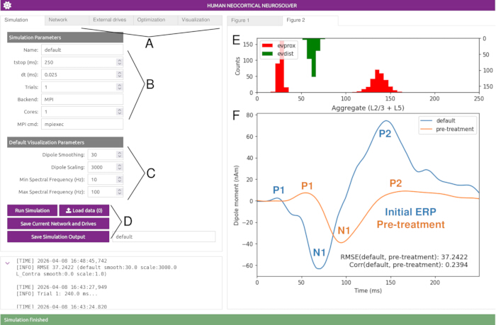
Figure 4. Comparison of canonical HNN simulated ERP waveform with empirical pre-treatment ERP. (A) Parameter categories accessible through graphical user interface (GUI) tabs. (B) Simulation parameters controlling simulation length and number of trials. (C) Visualization parameters controlling waveform display. (D) Simulation control panel for loading data, running simulations, and saving outputs. (E) Spike histograms showing distributions of exogenous drive inputs in the canonical ERP simulation. (F) Dipole waveform of the canonical ERP simulation (blue) overlaid with an empirical auditory ERP (orange) from Kohl et al.⁴³. The initial simulation does not fit the data, with misaligned peak timing and magnitude (Corr < 0.95). The experimental paradigm used to generate the empirical ERP is described in Kohl et al.⁴³: tones (1 kHz, 50 ms duration, 10 ms fade-in/out) were presented alternatingly to left and right ears, with inter-stimulus intervals of 0.8–1.2 s at 60 dB above subjective hearing level. Please click here to view a larger version of this figure.

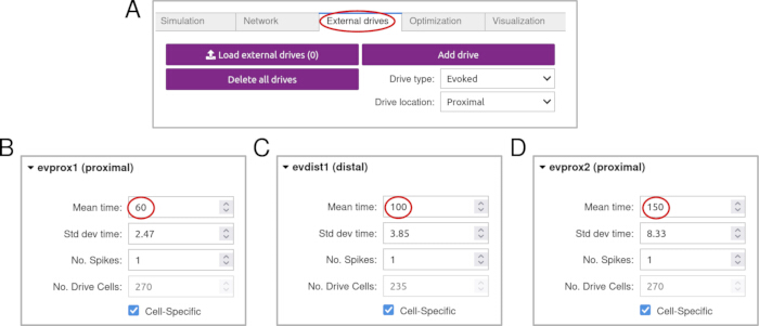
Figure 5. Modification of exogenous drive timing to align ERP peaks. (A) The “External drives” tab in the GUI, used to configure evoked inputs to the model. (B–D) Adjustment of mean time parameters for individual exogenous drives to align simulated ERP peaks with empirical data. Specifically, (B) proximal drive evprox1 aligned to ~60 ms, (C) distal drive evdist1 aligned to ~100 ms, and (D) proximal drive evprox2 aligned to ~150 ms. Adjusting the mean time parameter (highlighted) shifts the timing of simulated peaks and improves correspondence with the empirical waveform. These adjustments contribute to improved alignment and increased correlation with the target ERP (see Figure 7B). Please click here to view a larger version of this figure.

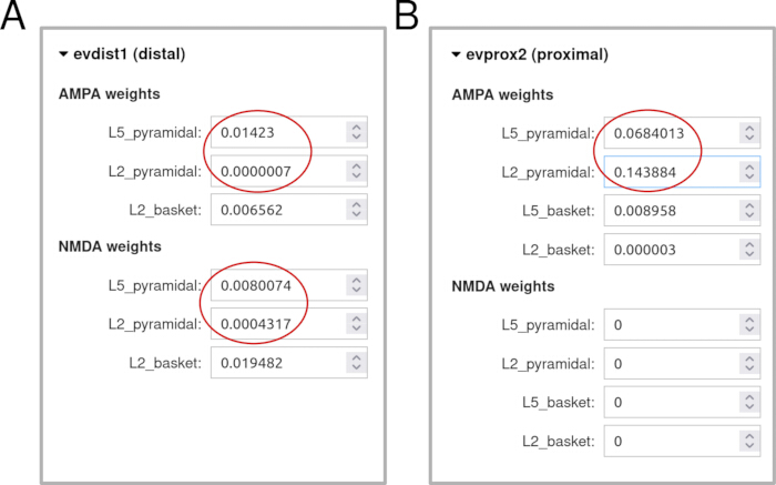
Figure 6. Modification of exogenous drive strength to adjust ERP peak magnitudes. (A and B) Synaptic weights for α-amino-3-hydroxy-5-methyl-4-isoxazolepropionic acid (AMPA) and N-methyl-D-aspartate (NMDA) receptors are modified through the “External drives” tab in the graphical user interface (GUI). (A) Adjustment of synaptic weights for the distal drive (evdist1), including AMPA and NMDA conductances targeting layer 2/3 (L2/3) and layer 5 (L5) pyramidal neurons. (B) Adjustment of synaptic weights for the proximal drive (evprox2), primarily affecting AMPA conductances in pyramidal neurons. In this example, synaptic weights are reduced by a factor of 10 relative to default values, resulting in decreased ERP peak magnitudes and improved agreement with the empirical waveform (see Figure 7C). Please click here to view a larger version of this figure.

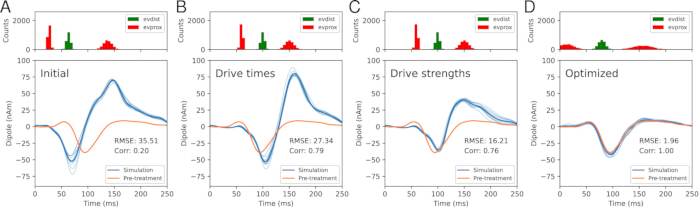
Figure 7. Manual tuning and optimization to fit model parameters. All simulations show 5 trials, with average ERP (dark blue) and individual trials (light blue). (A) Canonical ERP simulation (blue) overlaid with pre-treatment ERP (orange). (B) Adjustment of exogenous drive timing improves peak alignment. (C) Reduction of synaptic weights decreases peak magnitudes. (D) Automated optimization produces a close fit to the empirical waveform (Corr = 1.0), including increased variability in evoked drive timing. Please click here to view a larger version of this figure.

4. Establish pre-treatment model fit with parameter optimization

NOTE: Control of random seeding for optimization is not currently available in the GUI. For reproducible optimization runs, use the Python API. The associated code repository contains an example implementation (see code/baseline_optimization.py), where a fixed random seed can be set by passing a seed parameter to the optimization function (e.g., optim.fit(..., seed=123)).

NOTE: This example shows how to optimize targeted parameters to estimate single values that produce a close fit to the waveform using CMA-ES (not to be confused with SBI; both are approaches to fit model parameters, but the primary output of SBI is a distribution). An example of how to estimate distributions of parameters that can account for waveforms is shown in the Results section. For pre-treatment ERPs, start by optimizing exogenous drive parameters under the assumption that cell and local network connection parameters in the default HNN neocortical model are fixed. The multiscale prediction provided by HNN described in Step 7 provides targets for validation of this assumption. As new information becomes available to constrain model predictions, the HNN framework allows estimation of any set of parameters.

1. Open optimization settings
   1. Click the Optimization tab on the top left corner of the GUI (Figure 8A).
   2. Configure the settings of the optimization run, including the number of iterations, solver, and objective function.
      NOTE: The default optimization settings (Objective function = “dipole_corr”; Solver = “cma”) are appropriate for ERP waveforms. This objective function maximizes the correlation coefficient between simulated and empirical waveforms. Increase the maximum iterations if optimizing many parameters. The correlation coefficient is a scale-free measure; therefore, when using “dipole_corr”, adjust the scaling factor after optimization (Step 4.7.1). Alternatively, use “dipole_rmse” to minimize RMSE, in which case the scaling factor remains fixed.
   3. Click on the Max iterations textbox and enter 100.
2. Select parameters for optimization
   1. Click on the dropdown menu of an exogenous drive whose parameters will be optimized (Figure 8A and Figure 8B, red circle).
   2. Select the drive parameters to be optimized by clicking the checkbox under “Optimized against?” (Figure 8B).
3. Define parameter constraints
   1. Specify the range of parameter values explored by the optimizer by entering values into the Min and Max textboxes under Constraints (%) (Figure 8B).
      NOTE: Default values of 20% are suitable for simulations that already have a high correlation coefficient (Corr > 0.9). For example, applying a 20% range to a Mean time of 65.53 ms produces bounds of 52.42–78.64 ms. For poor initial fits, increase Min and Max percentages; however, the number of simulations required may increase significantly.
4. Run optimization
   1. Click the Run Optimization button (Figure 8A) to execute the optimization routine.
5. Save optimization results
   1. Click the Save Optimization History button (Figure 8A).
   2. Move the saved file to the project folder created in Step 2.5.
      NOTE: Optimization results can be stored and reused. The protocol may be paused at this stage and resumed by loading the saved optimization history.
6. Assess optimization quality
   1. Evaluate the quality of the optimization run.
      NOTE: When using correlation coefficient as the goodness-of-fit measure, a stopping criterion of Corr > 0.95 is recommended, as this generally reflects a simulated waveform that reproduces prominent peaks and troughs of the target ERP. Early stopping is not currently supported but is under development. Increase the number of iterations if the stopping criterion is not met but the loss continues to decrease every 10 iterations.
7. Determine next steps based on optimization outcome
   1. If a good fit to the pre-treatment ERP is achieved (i.e., Corr > 0.95), re-adjust the scaling factor to minimize RMSE and proceed to Step 5.
      NOTE: As described in Step 4.1, when “dipole_corr” is used as the objective function, re-adjust the scaling factor after optimization. In this example, the scaling factor was reduced from the default of 3000× (Figure 7A–7C) to 1000× (Figure 7D).
   2. If optimization fails to achieve a good fit to the pre-treatment ERP, return to Step 4.2 and perform troubleshooting by increasing the maximum iterations, improving the manually tuned starting point, or selecting alternative parameters to adjust.
      NOTE: Refer to the section “Troubleshooting when fitting parameters to data features” in the Discussion for a detailed explanation of troubleshooting steps.

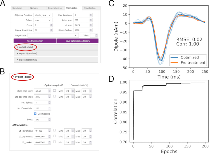
Figure 8. Optimization of exogenous drive parameters to improve fit to pre-treatment ERP. (A) Optimization tab in the GUI for configuring optimization parameters. (B) Selection of parameters and constraint ranges for optimization. (C) Example optimization result showing improved fit to empirical ERP data from Kohl et al.⁴³. (D) Optimization loss curve showing convergence after approximately 80 iterations. Please click here to view a larger version of this figure.

5. Establish post-treatment model fit

1. Start with the optimized pre-treatment ERP simulation. Manually tune and optimize the parameters of interest to fit the post-treatment ERP.
2. Load post-treatment empirical ERP waveform
   1. Load the post-treatment empirical ERP waveform from Step 1 into the GUI (same procedure as Step 3.2; Figure 9A).
3. Load optimized pre-treatment parameters
   1. Load the optimized pre-treatment ERP parameters from Steps 1–4 as a starting point (Figure 9A).
4. Perform manual tuning and optimization
   1. Perform manual hand tuning and parameter optimization (same procedures as Steps 3.2–3.11 and Step 4) on the parameters of interest identified in Step 1.7.
   2. Continue tuning and optimization until a high correlation (Corr > 0.95) between simulated and post-treatment ERP is achieved.
      NOTE: For illustrative purposes, in Figure 9B, hand tuning was applied to a signal-targeted parameter (decreased local network GABA_B maximal conductance), which produced a closer fit to the post-treatment data. Optimization was not performed to evaluate how well this parameter change accounts for the data. The “Representative Results” section describes how to estimate distributions of multiple parameters hypothesized to be post-treatment parameters of interest using SBI. SBI (detailed in Step 6) is recommended for rigorous investigations because it estimates distributions of parameters that account for an ERP waveform, enabling robust comparisons across parameter fits.
5. Save model configuration and compare parameters
   1. Save the model configuration and compare optimized values for parameters of interest between pre-treatment and post-treatment conditions (data not shown).
   2. Repeat Step 3.11 to export a .json file of model parameters. Move the file to the project folder created in Step 2.5.
   3. View exogenous drive parameters by clicking Load external drives (Figure 5A) and selecting either the pre-treatment or post-treatment network configuration file.
   4. View local network parameters by clicking Load local network connectivity (Figure 9C) and selecting either the pre-treatment or post-treatment network configuration file.
   5. Identify changes in parameter values across pre-treatment and post-treatment network configurations. Interpret these changes as model-based predictions of post-treatment biomarker mechanisms.

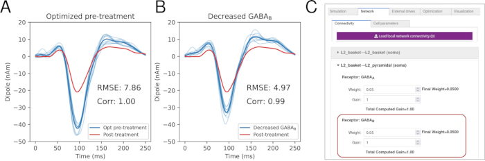
Figure 9. Evaluation of gamma-aminobutyric acid type B (GABA_B) synaptic strength as a mechanism of post-treatment EEG biomarkers. (A) Optimized pre-treatment simulation (blue) overlaid with post-treatment ERP (red), showing reduced peak magnitudes. (B) Reduction of GABA_B synaptic strength decreases N1 amplitude, suggesting a potential mechanism. (C) GUI panel showing where local GABA_B synaptic strength is modified. Please click here to view a larger version of this figure.

6. Perform uncertainty quantification with SBI and assess separability using the HNN-Python application programming interface

NOTE: SBI requires installation of a separate Python package⁶². Refer to the associated repository (https://github.com/ntolley/hnn_jove) for a code example detailing how to run parameter inference in HNN using the SBI software package. The code is organized to follow the steps in the subsequent protocol. A full discussion of applying SBI to the HNN model is provided in⁵⁵.

1. Install the SBI package
   1. Install the SBI package by running the following command in a terminal with the Python environment activated: pip install sbi.
2. Define prior parameter ranges
   1. Identify parameter ranges around the targeted subset of pre-treatment and post-treatment ERP parameters to create a bounded prior distribution for uncertainty quantification.
3. Generate training dataset.
   1. Define a parameter update function (same approach as parameter optimization).
   2. Fix the random seed for generating samples from the prior distribution to ensure reproducibility. If using NumPy for random sample generation, create a random number generator instance in the Python script (e.g., rng = np.random.default_rng(123)) and use this generator for sampling.
      NOTE: The associated code repository (https://github.com/ntolley/hnn_jove) provides an example of using a NumPy random generator in code/generate_simulations.py.
   3. Sample parameters from the prior distribution.
      NOTE: 10,000 samples were used to generate the representative results.
   4. Generate a dataset of simulated ERPs using the sampled parameter values.
4. Select summary statistics.
   1. Choose a summary statistic that characterizes the EEG waveform.
      NOTE: A summary statistic is any quantity that captures key features of an EEG waveform. Common choices include peak timing and magnitude. In this manuscript, principal component analysis (PCA) is used to extract summary statistics (i.e., the loadings of the first four principal components). See⁵⁵ for a complete discussion.
   2. Train SBI network
      NOTE: This tutorial uses the default training parameters (e.g. density_estimator=”maf”, training_batch_size=200, learning_rate=0.0005) distributed with the SBI package for the neural posterior estimator object. Training parameters are described in the SBI documentation (https://sbi.readthedocs.io/en/stable/api_reference/_autosummary/sbi.inference.NPE_B.html).
   3. Set the global PyTorch random seed to ensure reproducible training by including torch.manual_seed(0) in the Python script after importing torch.
   4. Train the SBI network to map parameter combinations to simulated ERP waveforms.
      NOTE: The trained SBI network is a Python object that accepts summary statistics from EEG data as input and outputs a distribution of parameters (posterior distribution). If training is successful, simulating parameters from this distribution in the HNN model produces EEG waveforms similar to the empirical data (posterior predictive check [PPC]).
   5. Generate posterior samples and evaluate fit
   6. Provide the experimental EEG waveform as a conditioning input to the trained network.
   7. Draw parameter samples from the posterior distribution conditioned on the experimental EEG waveform.
   8. Simulate the parameter samples drawn from the posterior distribution.
   9. Calculate the similarity between the simulated waveforms and the experimental EEG waveform provided as input.
      NOTE: This procedure is referred to as a PPC. A well-trained network produces simulations that closely match the empirical waveform (high correlation or low RMSE). If the PPC does not produce satisfactory simulations, two possibilities exist: (1) the hypothesized mechanisms do not account for the biomarker, requiring new hypotheses and updated prior distributions; or (2) the SBI network was not successfully trained. In this case, increase the training budget or modify the summary statistics.
   10. If simulated ERPs from the sampled parameter distributions fit the pre-treatment and post-treatment ERP (PPC with Corr > 0.95), proceed to Step 6.8. Otherwise, proceed to Step 6.7.
5. Troubleshoot SBI network training
   NOTE: A failed PPC indicates that the training parameters of the SBI network require modification. Refer to the section “Troubleshooting when fitting parameters to data features” in the Discussion for a detailed explanation.
   1. Increase the size of the training dataset.
   2. Modify the summary features.
   3. Select a different SBI architecture for training.
6. Visualize posterior distributions and assess separability
   1. Pass the array of parameter samples from Step 6.6.2 to the pairplot function and assign distinct colors to the distributions corresponding to each ERP condition.
      NOTE: The associated code repository demonstrates plotting functionality to reproduce Figure 10.
   2. Inspect the diagonal panels of the generated pairplot for non-overlapping distributions. Assess separability by calculating the OVL (Figure 10A). Parameters with highly separated distributions (OVL < 0.1) correspond to predicted mechanisms of action of the neurotherapeutic that change post-treatment relative to pre-treatment.
      NOTE: OVL is a metric that quantifies distribution separability in the range (0,1), where OVL = 0.0 indicates no overlap and OVL = 1.0 indicates complete overlap^54,55. Code to calculate OVL is provided in the associated code repository.

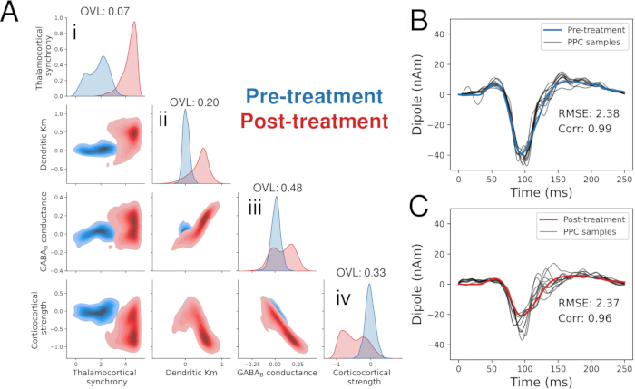
Figure 10. SBI for parameter uncertainty quantification and identification of neurotherapeutic mechanisms. (A) Pairplot visualization of parameter distributions estimated using SBI. Diagonal panels (i–iv) show univariate distributions for individual parameters, including (i) thalamocortical synchrony, (ii) dendritic K_m conductance, (iii) GABA_B conductance, and (iv) corticocortical feedback strength. Units for (i) are expressed as a multiplicative scaling factor of the default (pre-treatment) parameter value. Units for (ii-iv) are expressed as a multiplicative scaling factor of the default (pre-treatment) parameter value on a log scale. Distributions for pre-treatment (blue) and post-treatment (red) conditions demonstrate varying degrees of separability, with thalamocortical synchrony exhibiting the lowest overlap (overlap value, OVL = 0.07), indicating the strongest treatment-related effect. Off-diagonal panels show bivariate relationships between parameters. (B) Posterior predictive check (PPC) for pre-treatment ERP; simulated waveforms (black) closely match empirical data (blue). (C) PPC for post-treatment ERP; simulated waveforms (black) closely match empirical data (red). Please click here to view a larger version of this figure.

7. Perform examination, validation, and further model constraint

NOTE: This step provides examples of how to visualize elements of simulated activity in the GUI. These multiscale details provide targets to validate and inform model-derived predictions in follow-up experiments^7,47. This protocol does not provide guidance on selecting which predictions are best suited for validation experiments or how validation experiments should be performed (i.e., Step 7.3).

1. Load model parameters and run simulations
   1. Load model parameters optimized for pre-treatment and post-treatment conditions and run simulations.
      NOTE: Parameters from optimization in Steps 4–5 can be loaded and examined. Examples of how to export network parameters produced by SBI in Step 6 from the Python interface are included in the associated GitHub repository.
2. Examine multiscale predictions
   1. Examine multiscale predictions from simulated outputs.
   2. Plot cell-level spiking activity
   3. Click the Visualization tab (Figure 4A).
   4. Click the dropdown menu labeled Layout template and select Dipole Layers-Spikes.
   5. Under the Dataset dropdown, select the simulation results to be plotted.
   6. Click Make figure to visualize the spiking activity contributing to the dipole waveform.
      NOTE: Certain microcircuit features (e.g., LFP and CSD) are only available through the HNN-Python application programming interface (API). Code-based tutorials for these features are available on the HNN examples page (https://jonescompneurolab.github.io/hnn-core/stable/index.html).
3. Validate model predictions with empirical data
   1. Identify existing datasets and/or collect new empirical data (e.g., invasive electrophysiology, laminar MEG/EEG, and magnetic resonance spectroscopy) to test multiscale model predictions.
   2. Compare multiscale model predictions with empirical datasets.
   3. If multiscale predictions match empirical datasets, consider the model validated for the selected microcircuit feature.
   4. If multiscale predictions do not match empirical datasets, update the default HNN network by constraining it with new empirical data and return to Step 3.

Results

This section presents a scenario in which a neurotherapeutic with an unknown mechanism of action is investigated using the HNN modeling software. The goal is to use pre-treatment and post-treatment EEG signals to generate predictions on how the neurotherapeutic alters neural circuits. The results are presented for demonstration purposes to illustrate how HNN modeling can be applied to investigate neurotherapeutic mechanisms.

Developing mechanistic hypotheses underlying EEG ERP biomarkers (Step 1)

In this example, a hypothetical sensory ERP paradigm is used to examine how the neurotherapeutic alters the signal (Step 1). Figure 1A shows a pre-treatment auditory ERP (blue) alongside a hypothetical post-treatment ERP (red; see also Figure 9). The pre-treatment auditory ERP is experimentally recorded source-localized data from Kohl et al.⁴³, and the hypothetical post-treatment ERP is generated by scaling the pre-treatment waveform with a Gaussian-tapered window. As shown, the hypothetical neurotherapeutic produces a large decrease in the magnitude of the P1, N1, and P2 components relative to the pre-treatment ERP.

Note that in Kohl et al.⁴³, from which the pre-treatment ERP data was obtained, the HNN simulations used a model in which pyramidal neurons were enhanced with more realistic calcium channel dynamics than in the default HNN model. As a result, the simulation results in Kohl et al.⁴³, differ slightly from those shown here. The Kohl et al. 2020 model (and other updated HNN models) can be accessed through the Python API (https://jonescompneurolab.github.io/hnn-core/stable/generated/hnn_core.calcium_model.html#hnn_core.calcium_model). Access to such expanded models through the GUI is currently under development.

Next, identify model parameters representing treatment-related effects (i.e., parameters of interest) that are hypothesized to explain how the neurotherapeutic reduces the P1, N1, and P2 magnitudes (Steps 1.6–1.8). Broad categories of candidate neural mechanisms (and corresponding model parameters) include timing of exogenous synaptic inputs, local neuronal ion channel conductances, local synaptic connectivity, and exogenous synaptic connectivity (Figure 1B). In this example, candidate mechanisms from each category are evaluated using HNN to assess how changes in these parameters impact the simulated ERP.

Parameters of interest

1. Standard deviation of the first (thalamocortical) proximal drive (i.e., thalamocortical synchrony), representing variability in synchronization of initial feedforward sensory inputs.
2. Muscarinic potassium (K_m) channel conductance in layer 5 (L5) pyramidal neurons, controlling neuronal excitability, such that excitability decreases as conductance increases.
3. Local GABA_B receptor strength, corresponding to a slow inhibitory synapse delivered by interneurons to all cells in the local network.
4. Conductance strength of the feedback (corticocortical) distal drive, representing the strength of the ~100 ms sensory-evoked feedback input to AMPA and NMDA synapses in supragranular layers.

Establishing the pre-treatment ERP model fit (Steps 3–4)

Simulate the pre-treatment ERP by following Steps 3–4 (final pre-treatment simulation shown in Figure 8C). A successful result is indicated by a close match between simulated and empirical waveforms, as quantified by a high correlation coefficient and low RMSE.

Establishing the post-treatment ERP model fit (Step 5)

Use the pre-treatment ERP model as a starting point and apply manual tuning and parameter optimization to determine whether the parameters of interest can reproduce the empirical post-treatment ERP. A successful fit indicates that the hypothesized parameters are sufficient to explain treatment-related changes in the ERP waveform.

Uncertainty quantification with SBI (Step 6)

Due to parameter degeneracy inherent in biophysical models, uncertainty quantification using SBI (Step 6) is essential for making predictions about pre- to post-treatment parameter changes. A critical prerequisite for SBI is achieving accurate fits to pre-treatment and post-treatment ERPs (Steps 3–5). If accurate fits are not achieved, posterior samples generated by SBI may not reproduce the empirical waveforms, leading to unreliable predictions.

If a successful fit cannot be achieved in Steps 3–5, revise the selection of parameters of interest and their prior ranges before applying SBI.

In this example, SBI is applied only to the four post-treatment parameters of interest, while all other parameters are held fixed. Although applying SBI to a larger parameter set can improve robustness, it substantially increases computational cost (see Discussion).

SBI is used to estimate full parameter distributions that generate simulated ERPs closely matching target waveforms. Briefly, SBI is a Bayesian inference approach that trains a neural network to map model outputs to distributions of model parameters^52,53,55. The trained network is then applied to empirical waveforms to infer parameter distributions consistent with the data. This requires prior hypotheses on parameter ranges.

In this example, a uniform prior distribution is defined over the four parameters of interest: thalamocortical synchrony, pyramidal neuron dendritic Km conductance, local GABAB conductance, and corticocortical feedback strength. Prior bounds are defined as scalar multiples of default values: 0–5× for thalamocortical synchrony and 10⁻¹–10¹× for the remaining parameters.

Figure 10A shows the resulting parameter distributions for pre-treatment and post-treatment ERPs, visualized using a pairplot. Diagonal panels display univariate distributions, while off-diagonal panels display bivariate relationships. Mechanistic predictions correspond to parameters with strongly separated distributions between conditions.

Inspection of the univariate distributions shows that thalamocortical synchrony exhibits the greatest pre- to post-treatment separability (lowest OVL of 0.07) and increases following treatment (Figure 10A(iii), red). This indicates that the HNN framework predicts modulation of thalamocortical synchrony as a potential mechanism of action.

Posterior predictive validation

Validate inferred parameter distributions using a PPC. Generate independent parameter samples from the posterior distribution and simulate corresponding ERPs. A successful PPC is indicated when simulated waveforms closely match the empirical ERP.

As shown in Figure 10B and Figure 10C, both pre-treatment (Figure 10B, blue) and post-treatment (Figure 10C, red) waveforms closely match simulations generated from posterior samples (black), with correlation coefficients of 0.99 and 0.96, respectively (averaged over 10 independent samples). These results confirm that the inferred parameter distributions produce accurate waveform reconstructions.

An example of an unsuccessful PPC is provided in Supplementary Figure 1. The example follows the same structure as Figure 10 and uses the same trained SBI network; however, an alternate post-treatment waveform is used that is not well represented in the training set (e.g., ERP waveforms with a positive deflection at the N1 latency). The failed PPC is indicated in Supplementary Figure 1C, where the correlation coefficient is low (e.g., Corr < 0.95). Notably, the posterior distribution in Supplementary Figure 1A shows highly separated parameter distributions. Without performing a PPC, these results could be misinterpreted as meaningful differences between pre-treatment and post-treatment conditions. This example highlights the importance of conducting a PPC alongside interpretation of posterior distributions, as results from a failed PPC are unreliable and should not be further analyzed.

Model examination and validation (Step 7)

Using the HNN model, it is possible to directly inspect and visualize cell- and circuit-level activity, such as spiking, underlying each ERP simulation (Step 7.2.2). Figure 11A and Figure 11B shows simulated ERPs sampled from pre-treatment and post-treatment parameter distributions, alongside corresponding cell-specific spiking activity (Figure 11C and Figure 11D).

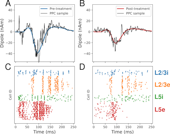
Figure 11. Cell-level spiking activity underlying EEG biomarker generation. (A) Pre-treatment ERP (blue) with a single posterior predictive simulation (black). (B) Post-treatment ERP (red) with a corresponding posterior predictive simulation (black). (C) Simulated spiking activity underlying the pre-treatment ERP. (D) Simulated spiking activity underlying the post-treatment ERP. Please click here to view a larger version of this figure.

The waveforms are visualized without smoothing to emphasize the contribution of spike timing to the current dipole. In experimental EEG signals, large neuronal populations produce spatially averaged signals that appear smoother. Because HNN simulates a smaller population (200 pyramidal neurons), smoothing is used to approximate larger-scale activity (>100,000 neurons).

A notable difference between conditions is reduced spiking activity in L5 pyramidal neurons following treatment (Figure 11C and Figure 11D, red dot). Note that Figure 11 shows a single sample from the posterior distribution; multiple samples should be analyzed to generate robust predictions. These results demonstrate that the hypothetical neurotherapeutic alters multiscale circuit activity, resulting in decreased P1–N1–P2 amplitudes.

Predictions such as these can be directly tested through invasive electrophysiology (e.g., high-density laminar probe recordings) or other imaging modalities (Step 7.3). Newly acquired data can then be used to further constrain model predictions. While this protocol focuses on fitting macroscale EEG data to infer microcircuit activity, the framework can also be applied in reverse by fitting microcircuit data (e.g., spiking, LFP/CSD) to infer macroscale EEG signals.

Supplementary Figure 1. Example of a failed posterior predictive check in the SBI workflow. Plots are organized identically to Figure 10. The pre-treatment data (blue) is identical to Figure 10. The hypothetical post-treatment data was generated identically as before (waveform multiplied with a Gaussian-tapered window), but transformed to produce a positive peak that is not well represented in the training set of HNN simulations. (A) Pairplot visualization of parameter distributions estimated using SBI. Diagonal panels (i–iv) show univariate distributions for individual parameters, including (i) thalamocortical synchrony, (ii) dendritic K_m conductance, (iii) GABA_B conductance, and (iv) corticocortical feedback strength. Distributions for pre-treatment (blue) and post-treatment (red) conditions demonstrate high separability for all parameters (OVL < 0.1). Off-diagonal panels show bivariate relationships between parameters. (B) Posterior predictive check (PPC) for pre-treatment ERP; simulated waveforms (black) closely match empirical data (blue). (C) PPC for post-treatment ERP; simulated waveforms (black) are highly dissimilar to the empirical data (red), with Corr < 0.95 indicating a failed PPC.Please click here to download this file.

Discussion

Computational neural modeling of EEG biomarkers may allow deeper insight into how CNS therapeutics reconfigure neural circuits and provide predictions on the biological processes underlying therapeutic effects. The workflow presented here demonstrates how a commonly measured EEG biomarker, auditory ERPs, together with biophysical modeling using the HNN, can be used as a window into the mechanisms by which a drug impacts neural activity. By linking macroscale EEG measurements to underlying cellular and circuit-level processes, this protocol provides a structured and hypothesis-driven framework for mechanistic interpretation. Importantly, the approach is not restricted to ERPs and can be extended to investigate other local EEG signals, including low-frequency neural oscillations^40,63 and transient spectral events^7,47,64, thereby broadening its applicability across electrophysiological biomarkers and experimental paradigms.

Compared to other frameworks for neural modeling of EEG, HNN offers a balance of model complexity and computational efficiency that is particularly advantageous for iterative hypothesis testing. For example, The Virtual Brain enables simulation of large-scale brain networks that generate spatiotemporal EEG signals^34,65. However, to achieve whole-brain modeling, neural activity is represented using reduced mathematical formulations, which eliminate detailed cellular features such as pyramidal neuron morphology and limit the ability to directly link model parameters to cellular mechanisms of drug action. Conversely, large-scale morphologically and physiologically detailed models can simulate EEG signals with high biological realism^66,67,68,69, but at a substantial computational cost, often requiring several hours of computation to simulate only a few seconds of neural activity. This computational burden can limit accessibility and slow the iterative process required for hypothesis generation and testing. HNN occupies an intermediate position (Figure 2), enabling simulation of localized neocortical circuits with sufficient biological detail to generate cell- and circuit-level predictions while maintaining computational efficiency (i.e., simulations on the order of seconds), making it well suited for integration into experimental workflows.

Despite these advantages, several limitations should be considered when applying EEG and biophysical neural modeling to study brain disease and drug mechanisms. The biophysical cell and circuit properties that generate EEG signals do not capture the full spectrum of biological processes affected by pharmacological interventions. For example, systemic or immunological responses may not directly influence EEG signals and therefore may not be reflected in the modeled outputs. In addition, mechanistic hypotheses are often derived from animal studies, which may not fully translate to human brain function, particularly in neuropsychiatric disorders where clinical outcomes are based on behavioral and cognitive assessments^70,71. Another important challenge is distinguishing between acute and chronic pharmacological effects. While acute drug-receptor interactions are relatively well characterized, the long-term adaptations induced by sustained drug exposure are less well understood and may not be fully captured in current modeling frameworks. Furthermore, the HNN model represents a single localized canonical neocortical network, whereas neurotherapeutics and CNS diseases often exert distributed effects across multiple brain regions. Although influences from other regions can be approximated through changes in the timing and strength of exogenous inputs, direct empirical characterization of these upstream or downstream circuits is often limited, which constrains model interpretation.

Parameter degeneracy represents a fundamental challenge in all biophysical neural models, as multiple parameter configurations can produce similar model outputs. In this protocol, SBI is used to address this issue by estimating distributions of parameters that generate ERP waveforms consistent with empirical data (Figure 10). This approach enables quantification of uncertainty in model parameters, providing a more robust framework for mechanistic interpretation than single-point estimates. However, for computational tractability, SBI is applied to a limited subset of parameters corresponding to hypothesized drug mechanisms, and assumptions regarding non-estimated parameters can influence the resulting network dynamics. Expanding inference to larger parameter spaces can be achieved using approaches such as sequential neural posterior estimation, which iteratively refines parameter estimates and enables exploration of higher-dimensional parameter distributions⁵² (>10 dimensions). In addition to probabilistic inference, incorporating independent experimental constraints can further reduce parameter uncertainty and improve the specificity of model predictions. Because EEG signals primarily reflect coordinated activity across cortical layers, complementary techniques such as invasive laminar electrophysiology—including measurements of cell spiking, LFP, and CSD—provide valuable information for constraining model solutions and refining mechanistic hypotheses.

Successful application of this protocol depends on careful execution of several critical steps. After identifying an ERP biomarker and installing the modeling framework (Steps 1–2), the primary requirement is achieving successful outcomes at each stage of the workflow (Figure 3). In Steps 3–5, this involves selecting and refining hypothesized parameters that can be manually tuned or optimized to achieve a close fit between simulated and empirical pre-treatment and post-treatment ERPs. If a satisfactory fit cannot be obtained, alternative parameters should be explored and iteratively tested. While repeated failures are unlikely given prior demonstrations of HNN’s ability to reproduce ERP features, persistent failure may indicate the need to modify the default network model or incorporate additional biophysical detail. Step 6 requires careful configuration of SBI, including appropriate selection of parameter ranges, summary statistics, and training parameters to ensure accurate estimation of parameter distributions. Upon successful completion of Step 6, the protocol yields both model-based predictions and associated uncertainty estimates. Step 7 is critical for validating these predictions, although the specific validation strategies depend on available experimental modalities. Potential validation approaches include laminar electrophysiological recordings to assess layer- and cell-specific spiking activity and LFP/CSD signals⁷, layer-resolved MEG/EEG measurements, magnetic resonance spectroscopy or positron emission tomography for assessing neurotransmitter systems, and diffusion tensor imaging for evaluating structural connectivity such as thalamocortical pathways.

Troubleshooting and customization are integral to adapting the protocol to different datasets and experimental contexts, particularly in Steps 3–6 where model parameters are fit to empirical data. Parameter optimization (Steps 4–5) may fail to converge to a high correlation (Corr > 0.95), in which case several adjustments can be made. These include modifying optimizer hyperparameters (e.g., increasing population size in the CMA-ES solver to improve robustness, with increased computational cost), refining scaling and smoothing parameters (e.g., testing smoothing values between 5 and 60 ms), and expanding the range of exogenous drive parameters or introducing additional drives to better capture waveform features. In some cases, optimized simulations may achieve high correlation while failing to capture lower-amplitude ERP features such as the P1 component; this can be addressed by applying stricter loss thresholds or weighting specific time windows to emphasize these features during optimization. For SBI (Step 6), failure of PPCs indicates that the simulated waveforms do not adequately reproduce the empirical data (Supplementary Figure 1). In such cases, the prior parameter distributions should be revised by expanding parameter ranges or including additional parameters, and the size of the training dataset may need to be increased. Additional improvements can be achieved by modifying summary statistics or selecting alternative SBI architectures. Finally, when validation in Step 7 fails, the default HNN network may require modification to include additional or alternative circuit elements. The modular design of HNN supports such extensions, allowing modification of synaptic connectivity and cellular properties through the GUI, and more advanced structural changes through the Python interface. For example, prior work has modified the default model to incorporate more detailed interneuron connectivity in frontal cortex⁴⁶, resulting in new testable predictions. The open framework of HNN facilitates sharing and reuse of expanded models, supporting continued refinement and validation across experimental contexts.

Materials

List of materials used in this article

Name	Company	Catalog Number	Comments
Anaconda Python	Anaconda, Inc.	N.A.	Python distribution; Python version ≥3.9 and <3.14
Computer workstation	N.A.	N.A.	Operating system: Windows ≥10, Linux, or macOS. Minimum recommended hardware: ≥16 GB RAM, ≥8 CPU cores
EEGLAB	EEGLAB Developers	N.A.	Optional MATLAB-based toolbox for EEG preprocessing and ERP analysis
FieldTrip	Donders Institute for Brain, Cognition and Behaviour, Radboud University	N.A.	Optional MATLAB-based toolbox for EEG/MEG analysis
Human Neocortical Neurosolver (HNN-core)	HNN Developers	N.A.	Biophysical neural modeling software; version ≥0.6.0 used in this study
MATLAB	MathWorks	N.A.	Required to run EEGLAB and FieldTrip (if used)
MNE-Python	MNE Developers	N.A.	Used for EEG preprocessing and source localization
NumPy	NumPy Developers	N.A.	Used for numerical computations and random number generation
Pixi (package/environment manager)	Prefix.dev	N.A.	Used for managing dependencies in the associated code repository
PyTorch	PyTorch Developers	N.A.	Used for training SBI neural networks and setting random seeds
SBI (Simulation-Based Inference) package	SBI Developers	N.A.	Python package for parameter inference and uncertainty quantification
Windows Subsystem for Linux (WSL2)	Microsoft Corporation	N.A.	Required only for Windows-based installations

References

- Gribkoff VK, Kaczmarek LK. The need for new approaches in CNS drug discovery: Why drugs have failed, and what can be done to improve outcomes. Neuropharmacology. 2017;120:11-19.
- Loo SK, Lenartowicz A, Makeig S. Research review: Use of EEG biomarkers in child psychiatry research—current state and future directions. J Child Psychol Psychiatry. 2016;57(1):4-17.
- McLoughlin G, Makeig S, Tsuang MT. In search of biomarkers in psychiatry: EEG-based measures of brain function. Am J Med Genet B Neuropsychiatr Genet. 2014;165(2):111-121.
- Douglas RJ, Martin KAC. Neuronal circuits of the neocortex. Annu Rev Neurosci. 2004;27:419-451.
- Harris KD, Shepherd GMG. The neocortical circuit: themes and variations. Nat Neurosci. 2015;18(2):170-181.
- Murakami S, Okada Y. Contributions of principal neocortical neurons to magnetoencephalography and electroencephalography signals. J Physiol. 2006;575(3):925-936.
- Sherman MA, et al. Neural mechanisms of transient neocortical beta rhythms: Converging evidence from humans, computational modeling, monkeys, and mice. Proc Natl Acad Sci U S A. 2016;113(33):E4885-E4894.
- Shin H, et al. The rate of transient beta frequency events predicts behavior across tasks and species. eLife. 2017;6:e29086.
- De Pieri M, et al. Pharmaco-EEG of antipsychotic treatment response: A systematic review. Schizophrenia. 2023;9(1):85.
- Hyun J, Baik M, Kang U. Effects of psychotropic drugs on quantitative EEG among patients with schizophrenia-spectrum disorders. Clin Psychopharmacol Neurosci. 2011;9(2):78-85.
- Jobert M, et al. Guidelines for the recording and evaluation of pharmaco-EEG data in man: The International Pharmaco-EEG Society (IPEG). Neuropsychobiology. 2012;66(4):201-220.
- Mandema JW, Danhof M. Electroencephalogram effect measures and relationships between pharmacokinetics and pharmacodynamics of centrally acting drugs. Clin Pharmacokinet. 1992;23:191-215.
- Leiser SC, Dunlop J, Bowlby MR, Devilbiss DM. Aligning strategies for using EEG as a surrogate biomarker: A review of preclinical and clinical research. Biochem Pharmacol. 2011;81(12):1408-1421.
- Wilson FJ, Danjou P. Early decision-making in drug development: The potential role of pharmaco-EEG and pharmaco-sleep. Neuropsychobiology. 2016;72(3-4):188-194.
- Klumpp H, Shankman SA. Using event-related potentials and startle to evaluate time course in anxiety and depression. Biol Psychiatry Cogn Neurosci Neuroimaging. 2018;3(1):10-18.
- Proudfit GH, et al. Depression and event-related potentials: Emotional disengagement and reward insensitivity. Curr Opin Psychol. 2015;4:110-113.
- Luck SJ, et al. A roadmap for the development and validation of event-related potential biomarkers in schizophrenia research. Biol Psychiatry. 2011;70(1):28-34.
- Salisbury DF, Collins KC, McCarley RW. Reductions in the N1 and P2 auditory event-related potentials in first-hospitalized and chronic schizophrenia. Schizophr Bull. 2010;36(5):991-1000.
- Kang E, et al. Atypicality of the N170 event-related potential in autism spectrum disorder: A meta-analysis. Biol Psychiatry Cogn Neurosci Neuroimaging. 2018;3(8):657-666.
- Modi ME, Sahin M. Translational use of event-related potentials to assess circuit integrity in ASD. Nat Rev Neurol. 2017;13(3):160-170.
- Horvath A, et al. EEG and ERP biomarkers of Alzheimer’s disease: A critical review. Front Biosci (Landmark Ed). 2018;23:183-220.
- Malver LP, et al. Electroencephalography and analgesics. Br J Clin Pharmacol. 2014;77(1):72-95.
- Preskorn SH, et al. Normalizing effects of EVP-6124 on event-related potentials and cognition: A randomized trial in schizophrenia. J Psychiatr Pract. 2014;20(1):12-24.
- Schwertner A, et al. Effects of subanesthetic ketamine on visual and auditory event-related potentials in humans: A systematic review. Front Behav Neurosci. 2018;12:70.
- Visser S, et al. Dose-dependent EEG effects of zolpidem provide evidence for GABAA receptor subtype selectivity in vivo. J Pharmacol Exp Ther. 2003;304(3):1251-1257.
- Okoroafor F, et al. Neurophysiologic biomarkers of invasive neuromodulation therapy for epilepsy. Neuromodulation: Technol Neural Interface. 2026;29(3):360-375.
- Maki-Marttunen T, et al. Biophysical psychiatry—how computational neuroscience can help understand the complex mechanisms of mental disorders. Front Psychiatry. 2019;10:534.
- Murray JD, Demirtas M, Anticevic A. Biophysical modeling of large-scale brain dynamics and applications for computational psychiatry. Biol Psychiatry Cogn Neurosci Neuroimaging. 2018;3(9):777-787.
- Cagney DN, et al. The FDA NIH biomarkers, endpoints, and other tools (BEST) resource in neuro-oncology. Neuro Oncol. 2018;20(9):1162-1172.
- Cecchi M, et al. Validation of a suite of ERP and QEEG biomarkers in schizophrenia. Schizophr Res. 2023;254:178-189.
- Dura-Bernal S, et al. NetPyNE, a tool for data-driven multiscale modeling of brain circuits. eLife. 2019;8:e44494.
- Linden H, et al. LFPy: a tool for biophysical simulation of extracellular potentials. Front Neuroinform. 2014;7:41.
- Neymotin SA, et al. Human Neocortical Neurosolver (HNN), a new software tool for interpreting MEG/EEG data. eLife. 2020;9:e51214.
- Sanz Leon P, et al. The Virtual Brain: a simulator of primate brain network dynamics. Front Neuroinform. 2013;7:10.
- Hamalainen M, et al. Magnetoencephalography—theory, instrumentation, and applications. Rev Mod Phys. 1993;65(2):413-497.
- Ikeda H, Wang Y, Okada YC. Origins of the somatic N20 and high-frequency oscillations evoked by trigeminal stimulation in the piglets. Clin Neurophysiol. 2005;116(4):827-841.
- Okada YC, Wu J, Kyuhou S. Genesis of MEG signals in CNS structure. Electroencephalogr Clin Neurophysiol. 1997;103(4):474-485.
- Bush PC, Sejnowski TJ. Reduced compartmental models of pyramidal cells. J Neurosci Methods. 1993;46(2):159-166.
- Jones SR, et al. Neural correlates of tactile detection. J Neurosci. 2007;27(40):10751-10764.
- Jones SR, et al. Quantitative analysis of MEG mu rhythm. J Neurophysiol. 2009;102(6):3554-3572.
- Law RG, et al. Thalamocortical mechanisms regulating beta events. Cereb Cortex. 2022;32(4):668-688.
- Fernandez Pujol C, Blundon EG, Dykstra AR. Laminar specificity of the auditory perceptual awareness negativity: A biophysical modeling study. PLoS Comput Biol. 2023;19(6):e1011003.
- Kohl C, Parviainen T, Jones SR. Neural mechanisms underlying auditory evoked responses. Brain Topogr. 2022;35(1):19-35.
- Lankinen K, Ahveninen J, Jas M, Raij T, Ahlfors SP. Neuronal modeling of cross-sensory visual evoked magnetoencephalography responses in the auditory cortex. J Neurosci. 2024;44(17):e1119232024.
- Kaplan L, et al. Modeling cortical dynamics using HNN [poster presentation]. Presented at: Society for Neuroscience Annual Meeting; San Diego, CA, USA; 2025.
- Diesburg DA, Wessel JR, Jones SR. Biophysical modeling of ERP generation. J Neurosci. 2024;44(20).
- Bonaiuto JJ, et al. Laminar dynamics of beta bursts. Neuroimage. 2021;242:118479.
- Ferrante M, Blackwell KT, Migliore M, Ascoli GA. Computational models of neuronal biophysics. Curr Med Chem. 2008;15(24):2456-2471.
- Geerts H, et al. Quantitative systems pharmacology for neuroscience drug discovery. CPT Pharmacometrics Syst Pharmacol. 2020;9(1):5-20.
- Geerts H, et al. Computational neuroscience and systems pharmacology. J Pharmacokinet Pharmacodyn. 2024;51(5):563-573.
- Kappenman ES, Luck SJ. ERP components: brainwave recordings. Oxford Handbook ERP Components. 2012;1:3-30.
- Goncalves PJ, et al. Training neural density estimators. eLife. 2020;9:e56261.
- Papamakarios G, et al. Normalizing flows for probabilistic modeling. J Mach Learn Res. 2021;22(57):1-64.
- Pastore M, Calcagni A. Measuring distribution similarities. Front Psychol. 2019;10.
- Tolley N, et al. Estimating parameters in neural models with SBI. PLoS Comput Biol. 2024;20(2):e1011108.
- Gramfort A, et al. MEG and EEG analysis with MNE-Python. Front Neuroinform. 2013;7:267.
- Sliva DD, et al. Transcranial stimulation and EEG perception. Front Psychol. 2018;9:2117.
- Thorpe RV, et al. Distinct neocortical mechanisms underlie human SI responses to median nerve and laser evoked peripheral activation. bioRxiv. 2021; Available at: https://doi.org/10.1101/2021.10.11.463545.
- Delorme A, Makeig S. EEGLAB toolbox. J Neurosci Methods. 2004;134(1):9-21.
- Oostenveld R, et al. FieldTrip software. Comput Intell Neurosci. 2011;2011:156869.
- Puce A, Hämäläinen MS. A review of issues related to data acquisition and analysis in EEG/MEG studies. Brain Sci. 2017;7(6):58.
- Tejero-Cantero A, et al. sbi: toolkit for simulation-based inference. J Open Source Softw. 2020;5(52):2505.
- Lee S, Jones SR. Distinguishing mechanisms of gamma frequency oscillations in human current source signals using a computational model of a laminar neocortical network. Front Hum Neurosci. 2013;7:869.
- Szul MJ, et al. Beta burst waveform motifs. Prog Neurobiol. 2023;228:102490.
- Hashemi M, et al. Bayesian virtual epileptic patient. Neuroimage. 2020;217:116839.
- Billeh YN, et al. Systematic integration of structural and functional data into multi-scale models of mouse primary visual cortex. Neuron. 2020;106(3):388-403.
- Borges FS, Moreira JV, Takarabe LM, Lytton WW, Dura-Bernal S. Large-scale biophysically detailed model of somatosensory thalamocortical circuits in NetPyNE. Front Neuroinform. 2022;16:884245.
- Markram H, et al. Reconstruction of neocortical microcircuitry. Cell. 2015;163(2):456-492.
- Hagen E, Næss S, Ness TV, Einevoll GT. Multimodal modeling of neural network activity: computing LFP, ECoG, EEG, and MEG signals with LFPy 2.0. Front Neuroinform. 2018;12:92.
- Geerts H. Of mice and men in CNS drug discovery. CNS Drugs. 2009;23(11):915-926.
- Nestler EJ, Hyman SE. Animal models of neuropsychiatric disorders. Nat Neurosci. 2010;13(10):1161-1169.
Reprints and Permissions