From Tissue to Morphometry: A Step-by-Step Golgi–Cox Workflow for Neuronal and Dendritic Spine Analysis in Adult Mice

Summary

This article describes a step-by-step method for Golgi–Cox staining in adult mice, covering solution preparation, tissue impregnation, cryoprotection, sectioning, development, and mounting. It emphasizes tissue preservation and homogeneous, low-background staining, enabling clear visualization of neuronal morphology. The method labels dendritic arbors and supports quantitative morphometric analysis of dendritic spines.

Abstract

Neuronal morphology analysis in health and disease is fundamental for understanding brain function and for assessing the effects of experimental interventions. Golgi–Cox staining remains a classical, yet highly relevant technique for visualizing complete neuronal arbors and dendritic spines. However, published protocols frequently differ in critical procedural steps and often lack essential methodological details, leading to substantial variability in staining quality and making laboratory standardization time-consuming and challenging. Here, a comprehensive, step-by-step Golgi–Cox protocol for adult mice is presented, encompassing the entire workflow from in vivo handling and tissue processing to imaging and morphometric data extraction. It details practical considerations and common pitfalls that influence impregnation efficiency, section integrity, and signal-to-noise ratio, and provide methodological guidance to improve reproducibility. Overall, this protocol enables reliable visualization and quantitative analysis of whole neurons, dendritic segments, and dendritic spines. It is anticipated that this resource will facilitate the implementation of Golgi–Cox staining with greater consistency, transparency, and technical rigor, while offering a clear framework for adapting the method to diverse laboratory settings.

Introduction

The overall goal of the Golgi–Cox staining method is to enable high-resolution visualization of complete neuronal morphology, including dendritic arbors and dendritic spines, in fixed brain tissue^1,2,3,4. This technique allows detailed structural analysis of individual neurons within complex neural circuits, making it particularly valuable for studies of synaptic plasticity, neurodevelopment, neurodegeneration, and experience-dependent structural remodeling^5,6.

The rationale for the development and continued use of Golgi-based methods lies in their unique ability to produce sparse and complete neuronal impregnation^1,2. Originally described by Camillo Golgi in 1873 and refined in 1891 by Cox^7,8, the method relies on the precipitation of silver chromate within a limited subset of neurons, enabling full morphological reconstruction without overlapping labeling³. The Golgi–Cox modification replaces the silver nitrate used in the original Golgi method with mercuric chloride, improving tissue penetration and consistency of staining². Compared to alternative neuronal labeling techniques such as fluorescent protein expression, viral tracing, or dye-filling approaches, Golgi–Cox staining offers several advantages. It does not require genetic manipulation, stereotaxic injections, or specialized microscopy equipment, and it permits visualization of dendritic spines with high contrast under brightfield microscopy^1,2. Although modern fluorescence-based methods provide cell-type specificity, Golgi–Cox staining remains particularly advantageous for unbiased morphological sampling^9,10 and for use in species or experimental conditions where transgenic tools are not available.

Within the broader literature, Golgi-based methods have been extensively employed to quantify dendritic spine density and morphology in studies of learning and memory⁵, stress and psychiatric disorders¹¹, aging¹², and neurodegenerative diseases such as Alzheimer’s disease^12,13,14. Its continued use across decades highlights its reliability for structural neuroanatomy². This method is particularly appropriate for researchers analyzing dendritic architecture and spine morphology in brain tissue when whole-cell visualization is required¹. It is well-suited for comparative morphological studies across experimental groups. However, investigators requiring cell-type specificity, live imaging, or molecular colocalization may benefit more from fluorescent or genetically encoded labeling approaches^9,10.

Protocol

Adult female wild-type B6129SF2/J mice (n = 3) were used in this study. However, similar staining can be accomplished using both sexes at the adult stage. All experimental procedures received previous Bioethics Committee approval. (#117.A, Institute of Neurobiology (INb), National Autonomous University of Mexico)

1. Preparation of solutions

CAUTION: Mercuric chloride is highly toxic and corrosive. Handle inside a chemical fume hood while wearing gloves, a lab coat, and eye protection. Dispose of waste in a labeled hazardous waste container. Potassium dichromate and potassium chromate are toxic and carcinogenic oxidizers. Handle inside a chemical fume hood and avoid skin contact or inhalation.

1. Prepare stock impregnation solutions
   1. Weigh 15 g of potassium dichromate. Dissolve it in 300 mL of double-distilled water to obtain a 5% (w/v) solution.
   2. Weigh 15 g of mercuric chloride. Dissolve it in 300 mL of double-distilled water to obtain a 5% (w/v) solution.
   3. Weigh 15 g of potassium chromate. Dissolve it in 300 mL of double-distilled water to obtain a 5% (w/v) solution.
   4. Wrap all containers in aluminum foil and store at room temperature, protected from light.
2. Prepare Golgi–Cox working solution
   1. Mix 50 mL potassium dichromate solution, 50 mL mercuric chloride solution, and 40 mL potassium chromate solution.
   2. Add 100 mL of distilled water and mix thoroughly.
   3. Incubate the mixture for 48 h at room temperature, protected from light.
   4. Allow the precipitate to settle. Use only the supernatant for tissue impregnation.
      ​NOTE: The Golgi–Cox solution can be stored for up to 1 month when kept protected from light. To reduce reagent waste and ensure solution freshness, prepare only the required volume of both the stock solutions and the final Golgi–Cox solution needed for the experiment. Prepare at least 23 mL per brain to obtain 20 mL usable supernatant after precipitate loss.
3. Prepare cryoprotectant solution
   1. Dissolve 300 g sucrose in 0.1 M phosphate-buffered saline (PBS), pH 7.4, prepared with anhydrous sodium phosphate dibasic, monohydrated sodium phosphate monobasic, and sodium chloride.
   2. Adjust the final volume to 1 L.
   3. Store at 4 °C for up to one week.

2. Tissue collection and impregnation

1. Perform Intracardiac perfusion
   1. Anesthetize the animal with sodium pentobarbital (252 mg/kg, i.p.). Confirm adequate depth of anesthesia by the absence of pedal withdrawal before proceeding.
   2. Perform intracardiac perfusion with approximately 30 mL of 0.1 M PBS (pH 7.4) until the effluent runs clear, ensuring complete removal of blood from the brain tissue. No fixative was used; the Golgi–Cox solution itself serves as the fixative in this workflow.
   3. Extract the brain carefully and rinse it in distilled water. Ensure that the brain is properly perfused and free of residual blood (Figure 1A).
2. Impregnate tissue
   1. Divide the brain into hemispheres or coronal blocks (~3 mm thickness) using a brain matrix to improve impregnation. Smaller tissue blocks facilitate more uniform impregnation and reduce variability, whereas larger samples may require longer incubation times and may exhibit less homogeneous staining.
   2. Place the brain in 10 mL Golgi–Cox solution. Protect from light.
      ​NOTE: A volume of 10 mL of Golgi–Cox solution is sufficient for a whole adult mouse brain. When using a single hemisphere or smaller coronal blocks (~3 mm thickness), the volume of solution may be reduced proportionally, provided that the tissue remains fully immersed. If the entire brain is used, it is recommended to section it while preserving the region of interest to ensure optimal reagent penetration and homogeneous impregnation.
   3. Incubate for 24 h at room temperature.
   4. Replace with 10 mL of fresh Golgi–Cox solution. Incubate for 10-14 days at 22–25 °C in the dark.
      PAUSE POINT: Store tissue in Golgi–Cox solution up to 15 days without major loss of viability.
      NOTE: Following Golgi–Cox impregnation, the brain develops a dark golden appearance and becomes highly fragile; therefore, handle it with care (Figure 1B). Using plastic tweezers for manipulation is recommended to avoid chemical reactions with steel materials.

3. Cryoprotection

1. Transfer the tissue into 10 mL cryoprotectant solution (30% sucrose (w/v) in 0.1 M PBS, pH 7.4, prepared in step 1.3).
2. Incubate for 24 h (4 °C).
3. At the same temperature (4 °C), replace with fresh cryoprotectant solution and incubate for at least 4–7 days.
   PAUSE POINT: Before sectioning, store tissue in cryoprotectant solution up to 3 weeks at 4 °C.

4. Embedding and sectioning

1. Embed tissue
   1. Prepare 8% (w/v) agarose in hot distilled water. Allow it to cool to approximately 40 °C.
   2. Place the tissue in embedding molds and orient appropriately.
   3. Pour agarose over the tissue and allow it to solidify for 1 h at room temperature or 30 min at 4 °C (Figure 1C).
   4. Trim excess agarose from the block (Figure 1D).
2. Section tissue
   1. Secure the agarose block onto the vibratome stage using adhesive. (Figure 1E)
   2. Fill the cutting chamber with cryoprotectant solution.
   3. Section tissue at 100–200 µm thickness. Thinner sections (e.g., 100–120 µm) are recommended for dendritic spine analysis to improve imaging resolution, whereas thicker sections (e.g., 150–200 µm) may be used for whole-neuron reconstruction. In this study, sections were cut at 120 µm (Figure 1F).
   4. Collect sections using a soft brush.
      NOTE: Record vibratome settings in the Table of Materials. Do not rinse the slides under any circumstances once the sections have been mounted. The sucrose will protect the tissue until the development step.

5. Mounting

1. Preparation of gelatin-coated slides
   1. Prepare a coating solution by dissolving 0.5 g of gelatin in 100 mL (0.5% w/v) of distilled water heated to boiling.
   2. Stir until the gelatin is completely dissolved and allow the solution to cool to room temperature.
   3. Add 0.05 g of chromium potassium sulfate (0.05% w/v) and mix until fully dissolved. Remove residual foam if necessary.
   4. Filter the gelatin solution through filter paper to remove undissolved particles and residual foam, ensuring a uniform coating of the slides.
   5. Wash glass slides with neutral detergent and water, rinse thoroughly, and then rinse with distilled water.
   6. Immerse slides in 96% ethanol until no visible droplets remain.
   7. Dry slides in an oven at 50–60 °C for 30 min or until completely dry.
   8. Dip slides into the gelatin solution and allow excess solution to drain.
   9. Place slides in an oven at 50–60 °C for 30 min or until completely dry.
   10. Repeat the coating and drying process at least five times to ensure proper adhesion.
   11. After the final drying step, allow slides to cool to room temperature in a dust-free environment (e.g., inside a chemical fume hood) and store them in a clean, closed container until use.
       NOTE: Prepare only the volume of gelatin solution required for the number of slides to be coated. Reagent quantities can be scaled proportionally while maintaining the specified concentrations (w/v).
2. Place sections onto gelatin-coated microscope slides using a soft brush
   NOTE: Use microscope slides coated with at least five layers of 0.5% gelatin. Prepare the slides freshly to ensure tissue integrity during development. Electrocharged slides were not tested in this protocol.
3. Soak absorbent paper with cryoprotectant solution and place it over the sections.
4. Press gently with the palm to eliminate air bubbles and ensure uniform contact between the tissue section and the gelatin-coated slide, promoting stable adhesion during subsequent processing.
   NOTE: Gentle pressure improves adhesion by maximizing contact between the section and the gelatin layer, reducing the risk of detachment during aqueous development.
5. Remove the paper carefully and allow slides to dry in the dark for 2–3 days at room temperature.
   NOTE: Drying in a low-humidity environment is critical for stable adhesion. Protection from light minimizes photochemical alterations of Golgi–Cox–impregnated tissue, which is sensitive to light due to the presence of chromate salts. In addition, residual agarose does not significantly interfere with the development process and can be observed surrounding the tissue in the developed section (Figure 2A). The presence of agarose facilitates safer handling of the tissue during mounting, as Golgi–Cox–impregnated tissue is highly fragile. If desired, excess agarose can be carefully removed manually after the sections have been mounted onto slides.
   PAUSE POINT: Keep the slides protected from light.

6. Development

CAUTION: Xylene is flammable and toxic by inhalation. Handle in a chemical fume hood and avoid open flames. Ammonia is corrosive and produces irritating vapors. Handle in a fume hood.

1. Rehydrate Sections
   1. Immerse slides in distilled water for 5 min.
   2. Transfer to fresh distilled water for 5 min.
   3. Immerse in 50% ethanol for 5 min.
      ​NOTE: The 50% ethanol step provides a gradual transition from aqueous conditions to dehydration, facilitating reagent penetration and helping preserve tissue integrity prior to the development step.
2. Develop staining
   1. Incubate slides in aqueous ammonia solution prepared by mixing 2 volumes of 25% ammonia with 1 volume of distilled water (2:1, v/v) for 8 min
   2. Wash in distilled water for 5 min.
   3. Wash again in distilled water for 5 min.
   4. Incubate in 5% (w/v) sodium thiosulfate in distilled water for 10 min in the dark.
   5. Wash in distilled water for 1 min.
   6. Wash again in distilled water for 1 min.
      ​NOTE: Complete the development process without interruption once started.
3. Dehydrate and Clear
   1. Immerse slides in 70% ethanol for 5 min.
   2. Immerse slides in 96% ethanol for 5 min.
   3. Immerse slides in 100% ethanol for 5 min.
   4. Transfer slides into xylene for at least 6 min.

7. Permanent mounting

1. Apply Permount® mounting medium (refractive index ~1.52) to each section.
   NOTE: The refractive index of the mounting medium should be compatible with oil-immersion objectives to ensure optimal image quality.
2. Place a coverslip carefully to avoid air bubbles.
3. Seal the edges with clear nail polish.
4. Allow slides to dry in the dark for 48 h at room temperature.

8. Imaging

NOTE: Imaging modalities and acquisition configurations vary by microscope brand; the optimal settings should be determined for each system.

1. Turn on the microscope.
2. Open the microscope software
3. Place a slide on the microscope stage.
4. Capture a 2D wide-view image of the brain section using a low magnification objective such as 1X/0.04 N.A. or 4x/0.10 (Figure 2A, B).

9. Imaging whole neurons

1. Capture high-resolution image stacks of the area containing the neuron of interest, using a 10x/0.25 N.A. or 20x/0.40 N.A. objective (Figure 2C).
   NOTE: Neurons selected for analysis should exhibit complete and homogeneous Golgi–Cox impregnation, with clearly defined dendritic arbors and minimal background staining. Cells with truncated processes, incomplete impregnation, overlapping structures, or high background signal should be excluded to ensure accurate morphometric analysis.
2. Focus the image and adjust camera settings, including the exposure and white balance.
3. Set the upper and lower boundaries for the image stack.
4. Set the step distance to 0.5 µm within the image acquisition window.
5. Capture the image stack using the software command for stack acquisition.
6. Repeat the above steps to capture every area of interest.
7. Save the data file and save all image files.TIFF format for external processing.

10. Imaging dendritic spines

1. Capture high-resolution image stacks of the area containing the neuron of interest, using a 63x/1.4 N.A. oil-immersion objective in an appropriate bright-field microscope (Figure 2D).
   NOTE: In the present manuscript, high-resolution images of dendritic spines shown in Figure 2D were obtained using the bright-field mode of a confocal microscope, Zeiss model LSM 780. However, other bright-field microscopes may serve to obtain 63x high-quality z-stack images, whose parameters should be standardized by each laboratory.
2. Apply 1–2 drops of immersion oil to the slide and place the objective over the slide, ensuring to make contact between the objective and oil.
3. Focus the image and adjust camera settings, including the exposure and white balance.
4. Set the upper and lower boundaries for the image stack.
5. Set the step distance to 0.3 µm within the image acquisition window.
6. Capture the image stack using the software command for stack acquisition.
7. Repeat the above steps to capture every area of interest
8. Save the data file and save all image files in TIFF format for external processing.
   ​NOTE: For steps 9 and 10. If the microscope is not equipped with a motorized stage for Z-stack acquisition, images can be collected manually by adjusting the micrometric focus. However, the spacing between optical sections may be less precise. In this case, Z-stacks can be reconstructed afterward in image processing software (e.g., ImageJ) from the acquired image sequence.

11. Morphometric analysis

NOTE: Various approaches and specialized software programs can be used for this purpose. Some free access tools for dendritic spine analysis include ImageJ or, as in this study, PyReconstruct¹⁵. For a more detailed description of PyReconstruct and its functionality for neuronal reconstruction and morphometric analysis, see the referenced source.

1. Procedure for dendritic spine morphometric analysis
   1. Once the file is opened in ImageJ, change the format to RGB by selecting Image > Type > RGB Color.
   2. Convert the Z-stacks into an image sequence in ImageJ: click File > Save As > Image Sequence. Save each image sequence in a separate folder for subsequent analysis. In PyReconstruct, load the image sequence by clicking File > New > From Images.
   3. A dialog window will appear, prompting the assignment of a name to the file (e.g., WTVR1N1 – Wild-Type Vehicle Mouse 1 Neuron 1).
   4. Three successive dialog windows will then appear. In the first window, enter the calibration value (µm/px). This information is available in the Z-stack metadata and can be accessed in ImageJ.
   5. In the second window, enter the thickness of each consecutive optical section (µm). Finally, the image series will begin loading automatically (Supplementary Figure 1A).
   6. Once the segment of interest has been identified, according to the inclusion criteria defined by the investigator, proceed with tracing to obtain quantitative data.
   7. Assign a distinct name and domain for each type of trace. Locate the domains in the lower panel, where they are represented by different colored geometric shapes (Supplementary Figure 1B).
   8. Draw a line corresponding to the desired sample length using the pencil tool. Then, generate a second trace through the Z-stack along the dendritic segment using the Z tool.
   9. Use the initial trace to determine the appropriate segment length and verify it under Lists > Z-trace List (Supplementary Figure 1B).
   10. Navigate through the Z-stack and identify dendritic spine heads with optimal focus. Using the pencil tool, trace the widest distal region of each spine head. Then, use the Z tool to trace the spine neck throughout the Z-stack (Supplementary Figure 1C, D). Repeat this procedure until all spine heads and necks within the selected dendritic segment have been traced.
2. Export spine head measurements
   1. Open the lists containing spine head width and length measurements. Access these under Lists > Trace List (for width) and Lists > Z-trace List (for length), respectively.
   2. Export the data to the desired location on the computer. Two separate Excel files will be generated, each containing the corresponding measurement data.
3. Classify spine morphology and calculate density
   1. Extract the width and length measurements of spine heads and necks from the previously generated Excel files.
   2. The data should be organized into the corresponding columns labeled Width and Length for morphological classification based on the following criteria¹⁶: filopodia (>2 µm), thin (< 2 µm), stubby (length-to-head width ratio ≤1), and mushroom (head width >0.6 µm). (Supplementary Figure 1E). Filopodia were rarely observed in the analyzed dendritic segments and were therefore not included in the analysis.
   3. The total number of spines per analyzed dendritic segment is determined at this stage, along with spine density (spines per linear µm), as well as the type and number of each spine subtype. The Excel template¹⁶ used for this analysis is available in is available in the referenced source. Using this method, basal dendritic spine density was quantified in the CA1 region of the hippocampus in 12-month-old female mice.
   4. Export quantified data and generate graphs with specialized scientific software applications designed for data analysis, graphing, and statistics. Here, the graph in Figure 3 was built with GraphPad Prism software.

Results

Tissue impregnation and sectioning
The Golgi–Cox protocol described here produced reliable and homogeneous neuronal staining in adult mouse brain tissue. After impregnation in Golgi–Cox solution, the brain acquired a characteristic dark golden coloration, indicating successful diffusion of the staining solution throughout the tissue. Vibratome sectioning preserved the structural integrity of neuronal somata and dendritic processes.

Neuronal visualization
Brightfield imaging revealed clearly defined neuronal cell bodies and dendritic arbors with minimal background staining. Individual neurons could be visualized in their entirety, including secondary and tertiary dendritic branches. At higher magnification, dendritic segments showed well-resolved spines, enabling morphometric analysis.

Quantitative analysis of dendritic spines
To demonstrate the applicability of this protocol for quantitative structural analysis, basal dendritic spine density was measured in pyramidal neurons from the CA1 region of the hippocampus in 12-month-old female mice. Dendritic spine morphometry was performed using tissue obtained from three animals. For each animal, six neurons were analyzed, and three dendritic segments (10 µm each) were evaluated per neuron. Spine density values were first averaged across segments for each neuron and subsequently averaged across neurons to obtain a single value per animal. Morphometric analysis was performed using open-source software (ImageJ-Fiji and PyReconstruct), enabling the extraction of geometric measurements and the classification of spine subtypes.

Representative quantification
Representative quantification of dendritic spine density and subtype distribution is shown in Figure 3. The analyzed dendritic segments showed a mean spine density of 1.20 ± 0.04 spines per µm of dendrite. Thin spines represented the most abundant subtype, followed by mushroom spines, while stubby spines represented a smaller proportion. These results demonstrate that the protocol provides sufficient staining quality and structural resolution for reliable dendritic spine morphometric analysis.

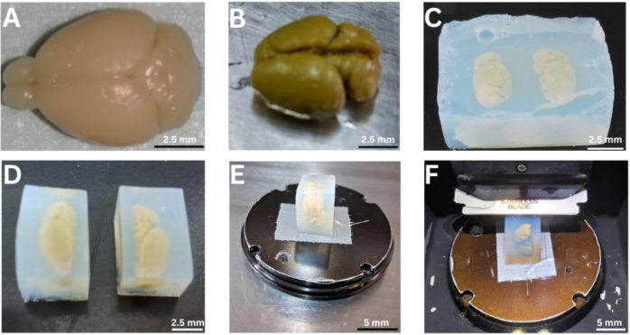
Figure 1: Tissue appearance and sectioning. Brain before and after 10 days of immersion in Golgi–Cox solution (A and B), hemispheres embedded in 8% agarose (C), agarose-embedded hemispheres prepared for vibratome sectioning (D), hemisphere mounted on the vibratome stage with coronal orientation for sectioning (E), and vibratome stage positioned inside the cutting chamber (F). Scale bars: A, B, C, D = 2.5 mm; E, F = 5.0 mm. Please click here to view a larger version of this figure.

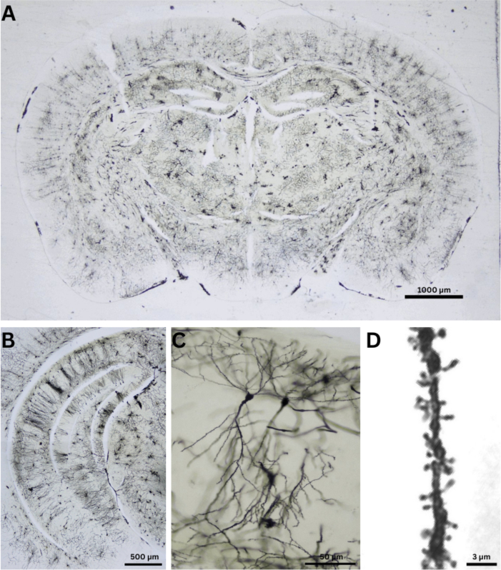
Figure 2: Golgi–Cox staining in the adult mouse brain. Neurons from multiple brain regions are uniformly and reliably stained using the Golgi–Cox protocol described here. (A) Representative whole-brain coronal section at low magnification. (B) Higher magnification image of one hippocampal hemisphere. (C) Representative hippocampal neuron showing the complete dendritic arbor. (D) Dendritic segment displaying clearly resolved dendritic spines. Sections cut at 120 µm. Scale bars: A = 1000 µm, B = 500 µm, C = 50 µm, and D = 3 µm. Please click here to view a larger version of this figure.

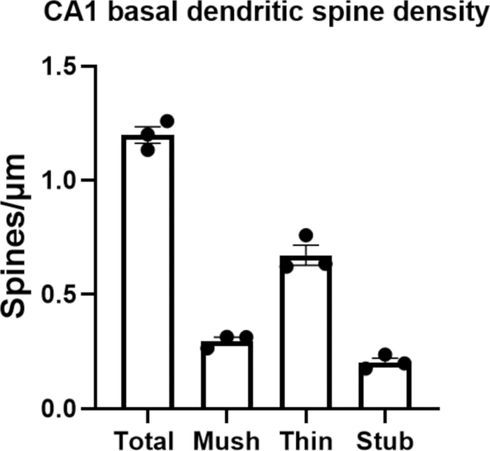
Figure 3: Quantification of dendritic spines in hippocampal CA1 neurons. Basal dendritic spine density was quantified in pyramidal neurons from the CA1 region of the hippocampus in 12-month-old female mice using the Golgi–Cox staining protocol described in this study. The graph shows total spine density (spines per µm) and the distribution of dendritic spine subtypes, including mushroom (Mush), thin (Thin), and stubby (Stub), as well as total (sum of mushroom, thin, and stubby) spines. Individual data points represent mean values per animal (n = 3), calculated by averaging measurements across neurons (n = 6) and dendritic segments (n = 3) within each animal. Bars represent mean ± SEM. Please click here to view a larger version of this figure.

Supplementary Figure 1: Workflow for dendritic spine morphometric analysis using PyReconstruct. (A) Z-stack image sequences are first imported into the software and calibrated using metadata parameters. (B) The dendritic segment of interest is then identified and traced to determine the length of the analyzed segment. (C) Dendritic spine heads are manually traced at the widest distal region using the pencil tool. (D) Spine necks are traced across the Z-stack using the Z-trace tool. (E) Geometric measurements are subsequently extracted and used to classify dendritic spine subtypes based on predefined criteria for head width and spine length.Please click here to download this file.

Discussion

The Golgi–Cox staining method remains one of the most widely used techniques for visualizing neuronal morphology and dendritic spines in fixed brain tissue^3,4. By impregnating a small, random subset of neurons, this method enables visualization of complete dendritic trees with minimal background staining. In the present protocol, the technique allowed clear visualization of hippocampal pyramidal neurons and their dendritic spines, enabling reliable morphometric analysis using bright-field microscopy and Z-stack imaging. Representative examples of staining quality and neuronal morphology obtained with this protocol are shown in Figures 1 and 3, where neuronal structures range from whole tissue sections to individual dendritic spines.

Several practical modifications and troubleshooting strategies can improve staining consistency. All Golgi–Cox solutions should be stored in darkness to maintain reagent stability. Although the typical incubation period in Golgi–Cox solution ranges from 10–14 days for sectioned tissue, longer incubation periods of up to 15 days can still yield viable staining results, although an increased presence of vascular staining may be observed. Similarly, tissue stored in cryoprotectant solution for extended periods before sectioning has been found to retain adequate staining quality. Alternative approaches, such as performing the developing step by flotation rather than slide-mounted tissue, are also possible; however, this approach requires careful handling because Golgi-impregnated tissue becomes extremely fragile.

Despite its advantages, several limitations of the Golgi–Cox method should be considered. The technique requires relatively long incubation periods and yields staining in only a small, random subset of neurons. In addition, Golgi staining may underestimate dendritic spine density compared to fluorescent labeling techniques such as intracellular dye filling. For example, comparisons between Golgi staining and Lucifer Yellow microinjection have shown that fluorescent methods can detect substantially higher numbers of dendritic spines¹⁷, although Golgi staining remains suitable for detecting relative differences in spine density across experimental conditions.

However, Golgi–Cox staining continues to be a widely used method for studying neuronal morphology because it allows detailed structural analysis without requiring transgenic labeling or fluorescent dyes^9,10. When combined with modern image acquisition and digital reconstruction tools such as PyReconstruct¹⁵, the method enables quantitative analysis of dendritic spine density and morphometric parameters. This makes the approach particularly valuable for studies investigating synaptic alterations associated with aging, neurodegenerative diseases, or experimental treatments. In particular, analysis of dendritic spine density in hippocampal neurons is widely used to investigate synaptic plasticity and structural synaptic changes associated with learning, memory, and neurodegeneration. Moreover, this method can be applied to study a wide range of physiological processes and pathological conditions.

Materials

List of materials used in this article

Name	Company	Catalog Number	Comments
Agarose	Life Technologies	15510-027	CAS 9012-56-6
Ammonia solution 25%	Merck	208380	CAS 1336-21-6. Hazardous.
Anhydrous sodium phosphate dibasic	Sigma-Aldrich	S3264	CAS 7558-79-4
Bright-field Microscope	Nikon	Eclipse Ci
Chromium potassium sulfate	Sigma-Aldrich	243361
Confocal Microscope	Zeiss	LSM 780
Digital balance	Accuris Instruments	W3200-1200
Embedding molds	Merck	E6032	Dimensions: 22x22 mm
Ethanol	Meyer	394
Experimental animals	The Jackson Laboratory	2124-01	B6129SF2/J mouse strain
Gelatin powder	Sigma-Aldrich	G2500
GraphPad Prism Software	GraphPad Software Inc.		Version 8.0.2
ImageJ Fiji Software	U.S. National Institute of Health		version 1.54p, https://imagej.net/software/fiji/downloads
Mercuric chloride	J.T. Baker	2594-01	CAS 7487-94-7. Hazardous.
Microscope Camera	Nikon	DS-Vi1
Microscope objective (10x)	Nikon	93183	Plan 10x/0.25 N.A.
Microscope objective (1x)	Nikon	93180	Plan UW 1x/0.04 N.A.
Microscope objective (20x)	Nikon	93184	Plan 20x/0.40 N.A.
Microscope objective (4x)	Nikon	93182	Plan 4x/0.10 N.A.
Microscope objective (63x)	Zeiss	420782-9900-799	Plan APO 63x/1.4 N.A. oil DIC
Microscope slides	Sigma-Aldrich	S8902
Monohydrated sodium phosphate monobasic	J.T. Baker	3818-05	CAS 10049-21-5
Nail Polish	SINFUL COLORS	BOLD COLOR	Transparent
Permount mounting media	Fisher Scientific	SP15-500
Potassium chromate	Productos Químicos Monterrey	2784	CAS 7789-00-6. Hazardous.
Potassium dichromate	Sigma-Aldrich	207802	CAS 7778-50-9. Hazardous.
PyReconstruct Software	University of Texas, Austin		version 1.19.0, https://github.com/SynapseWeb/PyReconstruct
Sodium chloride	Fermont	24912	CAS 7647-14-5
Sodium thiosulfate	Productos Químicos Monterrey	7291	CAS 7772-98-7. Hazardous.
Sucrose	J.T. Baker (Avantor)	4072-05	66.55° Specific rotation, ACS reagent
Vibratome	Leica Biosystems	VT1200S	SPEED 20 mm/s, AMPL – 0.60 mm
Xylene	CTR Scientific	CTR05128	CAS 1330-20-7. Hazardous.