Expansion-Assisted Hybridization Chain Reaction-smFISH and Immunohistochemistry in Drosophila Brain

Summary

This protocol describes an expansion-assisted HCR-smFISH and immunohistochemistry workflow for quantitative, cell-type-specific analysis of RNA and protein expression in the Drosophila brain, including imaging with light-sheet or confocal microscopy and automated quantification of nuclear and cytoplasmic transcripts.

Abstract

Quantitative, spatially resolved analysis of gene expression is essential for assessing cell-type-specific molecular profiles. In the Drosophila visual system, extensive genetic tools open a framework for direct evaluation of both RNA and protein levels in defined neuronal populations. Here, we present a step-by-step protocol that combines expansion-assisted HCR-smFISH (hybridization chain reaction single-molecule fluorescence in situ hybridization) with immunohistochemistry to enable quantitative analysis of cell-type-specific molecular profiles in genetically defined visual system neuronal types. The workflow is optimized for cells labeled with nuclear-localized or membrane-bound markers, allowing measurement of transcript and protein levels in the same neurons. Following tissue expansion, samples are imaged using light-sheet microscopy for rapid volumetric acquisition, with an alternative mounting and imaging workflow demonstrated for standard inverted laser scanning and spinning disc confocal microscopes. We further provide an automated segmentation algorithm that distinguishes nuclear and cytoplasmic transcripts, enabling analyses of transcriptional state and subcellular RNA localization. Practical guidance is provided on experimental parameters and common pitfalls affecting signal quality, tissue integrity, and quantitative performance. Representative applications include validation of cell-type-specific RNA interference by quantifying corresponding changes in RNA and protein levels. By enabling integrated RNA- and protein-level measurements with cell-type specificity, this approach provides a scalable strategy for hypothesis-driven molecular analysis and, in targeted contexts, a practical alternative to single-cell transcriptomic assays. This protocol provides a practical approach for validating cell-type-specific molecular perturbations while preserving the anatomical context of the intact Drosophila brain.

Introduction

The Drosophila melanogaster visual system has served as a powerful model for addressing a broad range of questions in developmental neuroscience, including neuronal differentiation^1,2, cell-type specification^3,4, and molecular logic of brain wiring^5,6,7. This progress has been driven by an unusually rich experimental toolkit, including large collections of cell-type-specific genetic driver lines^8,9,10, recent comprehensive connectomic reconstructions^10,11,12, and increasingly detailed single-cell transcriptomic^13,14 and multiomic¹⁵ datasets. Together, these resources define neuronal types in a multimodal fashion and enable precise genetic manipulations. As a result, the field can now generate increasingly predictive hypotheses about how specific genes regulate neuronal identity, connectivity, and function¹⁶.. While single-cell RNA sequencing provides powerful insights into transcriptional states, RNA abundance does not always predict protein expression¹⁷, and many perturbation experiments ultimately require direct, quantitative measurement of both RNA and protein in the same neurons.

Single-molecule fluorescence in situ hybridization (smFISH)^18,19 enables quantitative measurement of transcript abundance with cellular and subcellular resolution while preserving anatomical context. The combination of smFISH with expansion microscopy^20,21,22 has further extended its utility to intact brains by physically enlarging tissue within a swellable hydrogel, thereby reducing molecular crowding, improving optical access, and increasing effective spatial resolution. When paired with hybridization chain reaction (HCR)-based signal amplification²³, expansion-assisted smFISH allows robust detection of discrete transcripts throughout thick neural tissue and supports whole-brain imaging using either light-sheet or confocal microscopy.

A range of in situ RNA imaging approaches has been applied to the Drosophila brain, reflecting different experimental priorities. Expansion-assisted iterative HCR-FISH has enabled whole-brain, spatially resolved RNA detection²⁴. In parallel, non-expansion whole-mount FISH approaches have been used for RNA measurements in genetically labeled neurons, including HCR-based activity-mapping strategies centered on immediate early genes²⁵ and segmentation-based transcript counting workflows using membrane-bound genetically encoded markers²⁶. Commercial probe-based methods such as RNAscope have further enabled multiplex RNA detection in whole brains, often combined with immunohistochemistry to identify targeted cell populations²⁷. Together, these approaches establish that spatially resolved RNA analysis in the fly brain is technically feasible. However, hypothesis-driven perturbation experiments impose a more specific set of requirements that are not fully addressed by any single existing workflow. Many methods prioritize either multiplex discovery-style transcript mapping, activity-state profiling, or RNA quantification alone, with immunostaining typically serving as a cell identifier rather than as a matched readout of the perturbed protein, or being applied in the absence of genetic cell-type assignment²⁸. In addition, routine applications would benefit from compatibility with multiple imaging platforms and from automated, scalable analysis pipelines.

Here, we present an integrated, step-by-step workflow for the Drosophila visual system that combines expansion-assisted HCR-smFISH with immunohistochemistry performed prior to expansion, enabling paired measurement of RNA and protein levels in the same neurons within the same biological specimen. Building on the FlySeg framework²⁹ we previously developed, we provide an automated quantification pipeline for nuclear segmentation and transcript counting that distinguishes nuclear and cytoplasmic puncta, supporting both total-expression measurements and transcriptional-state–sensitive analyses. The protocol is demonstrated on both a light-sheet microscope and two confocal systems with alternative mounting and imaging workflows. Finally, we illustrate the utility of the integrated RNA–protein readout with a representative perturbation-validation experiment (i.e., RNAi-mediated knockdown of a defined target), providing practical guidance on parameters and pitfalls that affect signal quality, tissue integrity, and quantitative performance.

This protocol generally builds on the previously described²⁴ EASI-FISH framework for whole-brain RNA detection in Drosophila, and retains its core principles of RNA anchoring, hydrogel expansion, and HCR-based signal amplification. The present protocol extends and refines this approach by integrating immunohistochemistry prior to expansion to enable matched RNA and protein measurements in the same neurons, by revising multiple processing and handling steps throughout the workflow to improve robustness and reproducibility, by providing practical mounting and imaging strategies for both light-sheet and conventional inverted confocal microscopes, and by incorporating automated soma segmentation and transcript quantification with explicit separation of nuclear and cytoplasmic RNA pools.

This workflow is best suited for targeted experiments in which the goal is to quantify defined RNA and protein readouts in genetically identified neurons while preserving anatomical context. It is particularly useful for validating molecular perturbations when the goal is to measure up- or down-regulation of a defined gene or a small set of candidate genes, compare expression across genotypes or developmental stages, or assess transcriptional state through nuclear versus cytoplasmic transcript localization. It is less suitable for unbiased transcript discovery or high-plex whole-brain expression mapping, where single-cell sequencing, spatial transcriptomics, or iterative multiplexed FISH approaches may be more appropriate.

Protocol

Ethics statement

This protocol uses Drosophila melanogaster. No vertebrate animals or human subjects were used. Hence institutional animal care and use committee approval was not required.

NOTE: Use RNase-clean technique throughout. Wear gloves, wipe down surfaces and tools with RNase decontamination solution, and prepare all solutions with RNase-free water.

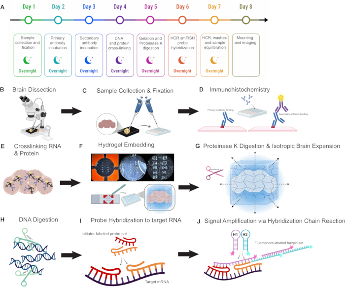
Figure 1. Step-by-step workflow of the sample preparation protocol (A) Schematic timeline of the protocol, indicating the approximate day-by-day progression and overnight incubation steps. (B–J) Schematic overview of the major sample preparation steps, from brain dissection and fixation through immunohistochemistry, RNA/protein crosslinking, hydrogel embedding, digestion, probe hybridization, and HCR signal amplification.Please click here to view a larger version of this figure.

1. Brain dissection, fixation, and immunohistochemistry (Day 1–3)

NOTE: Perform all steps in a Terasaki-style multi-well plate unless otherwise noted. Use 10 µL per well for incubations and washes. Maintain humidity by placing a moistened laboratory wipe in one corner of the plate.

CAUTION: Paraformaldehyde and glyoxal fixatives are toxic/irritant. Handle in a fume hood and wear appropriate PPE.

1. Dissect brains in ice-cold S2 insect medium. Transfer brains into wells, up to 10 brains per well (Figure 1B–C).
   NOTE: For the representative experiments shown here, 72 h-old pupal brains were used.
2. Replace S2 medium with 10 µL fixative per well, exchange once.
3. Fix in Addax acid-free glyoxal with 5% (w/v) sucrose overnight at 4 °C (Figure 1C).
4. Wash brains 3× in 10 µL PBST (0.5% Triton X-100 in PBS) for 10 min each at room temperature.
   CAUTION: Triton X-100 is an irritant; avoid skin and eye contact.
5. Incubate brains in 10 µL primary antibody solution (in PBST, at the dilutions listed in the Table of Materials) for 24 h at 4 °C. (Figure 1D).
6. Wash brains 3× for 10 min in 10 µL PBST at 4 °C. For each wash, replace the solution once midway through the incubation (two exchanges per wash).
7. Incubate brains in 10 µL secondary antibody solution (in PBST, at the dilutions listed in the Table of Materials) for 24 h at 4 °C (Figure 1D).
   NOTE: Protect samples from light.
8. Wash brains 3× for 10 min in 10 µL PBST at 4 °C. For each wash, replace the solution once midway through the incubation (two exchanges per wash).
   NOTE: Use primary and secondary antibody concentrations 2–3x higher than standard whole-mount immunohistochemistry concentrations
   PAUSE POINT: Store brains in 10 µL 1× PBS at 4 °C for up to 96 h.

2. Covalent anchoring of RNA and proteins (Day 4) (Figure 1E)

CAUTION: RNA-anchoring alkylators and AcX are hazardous (toxic/irritant; some are suspected carcinogens). Prepare and handle solutions in a chemical fume hood with appropriate PPE. Collect all waste as hazardous chemical waste.

1. Incubate brains in 10 µL of 20 mM MOPS buffer (pH 7.7) for 20 min at 37 °C.
2. Prepare anchoring solution by mixing 49.5% (v/v) 20 mM MOPS, 49.5% (v/v) Melphalan stock (2.5 mg·mL^-1 in DMSO), and 1% (v/v) AcX stock (10 mg·mL^-1 in DMSO). This yields final concentrations of 1.24 mg·mL^-1 melphalan and 0.10 mg·mL^-1 AcX.
3. Replace MOPS with 7–8 µL anchoring solution per well, exchange the solution once, and incubate overnight at 37 °C in the dark.
   NOTE: Use 7–8 µL to minimize overflow and cross-well mixing while maintaining full sample coverage.

3. Gelation (embedding brains in a hydrogel) and proteinase K digestion (Day 5)

CAUTION: Acrylic monomers, APS, and TEMED are irritants/toxic. Handle with PPE; prepare volatile/exothermic components in a fume hood.

1. Attach a 0.5 mm-thick adhesive silicone gasket to an uncharged glass microscope slide (Figure 1F, bottom left), press firmly to ensure full contact and sealing.
2. Add 200 µL of poly-L-lysine solution to the chamber and spread evenly to coat the surface, incubate at room temperature for 5 min, and remove the solution with a pipette.
3. Allow the poly-L-lysine to evaporate fully until the surface is visibly dry.
   NOTE: Poly-L-lysine evaporation is slow. For reliable results, prepare chambers in advance and allow them to dry overnight in a dust-free environment. Alternatively, dry chambers in a 37 °C incubator for ≥ 1 h on the day of use.
4. Wash brains 2× in 10 µL 1× PBS for 10 min each at room temperature.
5. Prepare gel monomer solution and add polymerization reagents immediately before use by mixing monomer solution with 4HT, TEMED, and APS (make fresh) at a ratio of 47:1:1:1. The final gelation solution contains 1 M sodium acrylate, 14% acrylamide, 0.1% bis-acrylamide, 1× PBS, 0.01% 4HT, 0.2% TEMED, and 0.2% APS.
6. Vortex briefly and keep the final gelation solution on ice. Use the solution immediately.
7. Incubate brains in 10 µL cold gelation solution for 15 min on ice.
8. During pre-equilibration, using a new razor blade, cut one narrow channel on each side of the silicone gasket to allow air to escape during filling (Figure 1F, top left)
9. Using a pipette tip, transfer brains into the prepared gelation chamber, ensuring each brain remains submerged in gelation solution at all times.
   CAUTION: After anchoring and equilibration, brains become highly adhesive and readily stick to plastic surfaces. To prevent sample loss, use wide-bore pipette tips or trim the end of a standard tip to widen the opening.
10. Remove the protective liner from the surface silicone gasket adhesive and gently place a clean 1.5H glass coverslip over the chamber, avoiding trapped air bubbles.
11. Slowly pipette 200 µL of freshly made gelation solution into the chamber through one of the side channels, until the chamber is completely filled.
12. Place the sealed chamber in a dark container and incubate at 37 °C for 2 h.
    NOTE: Place water-moistened laboratory wipes) inside the container. Ensure that the slide does not come into direct contact with liquid water.
13. Prepare digestion buffer consisting of 50 mM Tris-HCl (pH 8.0), 500 mM NaCl, 1 mM EDTA, and 0.5% (v/v) Triton X-100 in RNase-free water.
14. Immediately before use, add Proteinase K at 1:100 from a 20 mg·mL^-1 stock to a final concentration of 0.2 mg·mL^-1.
    CAUTION: Proteinase K is an irritant and should be handled with gloves; avoid inhalation and skin contact.
15. Allow the slide to cool at room temperature for 5 min before removing the coverslip. Trim the gel with a scalpel into a rectangular shape using single, straight cuts. Minimize the excess gel volume surrounding each brain (Figure 1F, top right).
16. Place each trimmed gel into an individual well of a 24-well plate containing 1000 µL digestion solution. Ensure gels are fully submerged.
17. Seal the plate with Parafilm and incubate overnight at room temperature on an orbital shaker at 0.11 g (Figure 1G).

4. DNase digestion and HCR-smFISH probe hybridization (Day 6)

1. Carefully aspirate the digestion solution using a pipette positioned at the edge of the well to avoid contacting or deforming the gel.
2. Wash gels 3× with 500 µL 1× PBS for 15 min each at room temperature on an orbital shaker at 0.11 g.
   PAUSE POINT: Store gels submerged in 500 µL 1× PBS at 4 °C for up to 7 days before proceeding.
3. Prepare 500 µL DNase working solution per gel by diluting DNase I stock from the QIAGEN RNase-Free DNase Set 1:10 in RDD buffer. The final working solution contains approximately 0.27 Kunitz units·µL^-1.
4. Incubate gels in 500 µL DNase working solution for 2 h at 37 °C with gentle rocking (Figure 1H).
5. Wash gels 4× with 500 µL RNase-free 1× PBS for 15 min each at room temperature.
6. Equilibrate gels in 500 µL pre-warmed probe hybridization buffer for 30 min at 37 °C
7. Dilute HCR smFISH probe stock (1 µM; Molecular Instruments) 1:300 in probe hybridization buffer to a final concentration of ~3.3 nM. Mix by vortexing
8. Replace equilibration buffer with 500 µL probe mix per gel and incubate overnight at 37 °C on an orbital shaker at 0.11g (Figure I).
   CAUTION: Probe hybridization buffers contain formamide, which is toxic. Use gloves and avoid inhalation.

5. Hybridization Chain Reaction (Day 7) (Figure 1J)

1. Wash gels 3× with 500 µL pre-warmed probe wash buffer for 30 min each at 37 °C on an orbital shaker at 0.11 g.
   CAUTION: Probe wash buffers contain formamide, which is toxic. Use gloves and avoid inhalation.
2. Wash gels 3× with 500 µL 1× PBS for 30 min each at room temperature on an orbital shaker at 0.11 g.
3. Leave gels in 1 mL 1× PBS overnight at room temperature on an orbital shaker at 0.11 g.
   NOTE: An extended overnight wash improves signal-to-noise ratio by reducing off-target probe binding and background puncta. For same-day processing, proceed directly to HCR amplification.
   PAUSE POINT: After post-hybridization washes, store gels in 1 mL 1× PBS at room temperature or 4 °C for up to 96 h before HCR amplification.
4. Replace PBS with 500 µL amplification buffer (previously equilibrated to room temperature) per well and incubate for 30 min at room temperature on an orbital shaker at 0.11 g.
5. For each probe set, dilute hairpins h1 and h2 (3 µM stock; Molecular Instruments) in amplification buffer 1:100 buffer (30 nM final concentration). Prepare 350 µL of diluted hairpin mix per well.
6. Heat diluted hairpin solutions in PCR tubes at 95 °C for 90 s in a thermal cycler or heat block. Use 100 µL total volume per tube to ensure uniform heating and temperature equilibration.
   NOTE: HCR guidelines commonly recommend snap-heating hairpin h1 and h2 separately and combining them only after cooling, Alternatively, combine H1 and H2 before snap-heating when simplified handling is required.
7. Allow hairpins to cool to room temperature for 10 min in the dark without disturbance.
8. Remove amplification buffer and add 350 µL hairpin mix per well.
9. Incubate gels for 2 h at room temperature in the dark on an orbital shaker at 0.11 g.
10. Wash gels 3× with 500 µL 5× SSCT for 10 min each at room temperature on an orbital shaker at 0.11 g.
11. Recover hairpin solutions after amplification, protect them from light, and store them at -20 °C for reuse.
12. Transfer gels to 500 µL 1× PBS and wash 3× for 30 min at room temperature.
13. Store gels in 500 µL 1× PBS at 4 °C, protected from light.
    PAUSE POINT: Amplified gels can be stored for up to 2 weeks before imaging with minimal signal loss.

6. Preparation, mounting, and imaging of expanded samples (Day 8) (Figure 2)

1. Incubate gels in 1× PBS containing DAPI (1:1000) overnight at 4 °C on an orbital shaker at 0.11 g.
2. Use brief UV illumination to visualize the brain within the gel. Orient the sample and trim excess gel as needed.
   CAUTION: UV illumination is used during sample positioning and mounting. Wear appropriate eye protection.
3. Mount samples in 1× PBS supplemented with DAPI (1:1000) using the appropriate configuration for the selected imaging platform (see Table 1).
4. Allow samples to equilibrate for at least 1 h before acquisition.
5. Use water-immersion objectives with sufficient working distance to image through the expanded gel.
6. Image samples using light-sheet microscopy, laser-scanning confocal microscopy, or spinning disk confocal microscopy. Representative platform-specific mounting and acquisition parameters used in this study are summarized in Table 1.
   NOTE: Following imaging, probes and HCR hairpins can be removed by DNase digestion as described above. Gels can then be subjected to additional rounds of probe hybridization and HCR amplification.

Platform	Sample visualization, mounting, and locating	Objective / detector	Representative acquisition settings
Zeiss Lightsheet 7	Use brief UV illumination to visualize brain position in the gel. Trim excess gel and orient each brain toward the detection objective. Place 5–6 gels on a 1 × 1 cm poly-L-lysine-coated coverslip with gels facing outward (Figure 2A). Attach the coverslip to the LS7 sample holder using a small drop of UV-curable adhesive; turn off the UV lamp before applying adhesive. Mount in the LS7 chamber and locate brain regions using live view in ZEN Black.	20×/1.0 NA water-immersion detection objective; 2.5× optical zoom (50× total magnification).	z-step, 0.4 μm at 2.5× zoom and 2× expansion. Pivot scanning enabled. Exposure, 50 ms for all channels. Lasers: 405 nm at 5%, 488 nm at 2%, 561 nm at 8%. Emission: 420–470 nm, 505–545 nm, 570–620 nm.
			(Figure 2C, left)
Nikon Ti2-E AXR NSPARC laser-scanning confocal	Use brief UV illumination to visualize the brain within the gel. Orient a single gel so that the brain faces downward toward the inverted objective. Transfer to a glass-bottom imaging dish filled with 1× PBS + DAPI (Figure 2B). Locate the brain with a 4× objective, identify ROIs with a 20× objective, and register X-Y positions in NIS-Elements. Add immersion medium, revisit registered ROIs, and bring them into focus.	40× long-working-distance water-immersion objective (Nikon CFI APO LWD 40× WI, 1.15 NA Lambda S, 0.61 mm working distance); NSPARC detector in super-resolution mode.	Galvanometer scanning, 2048 × 2048 pixels, 1.6 μs/pixel, 8.0× zoom. Lasers: 488 nm at 2%, 640 nm at 20%. Emission: 502–546 nm and 666–732 nm.
			(Figure 2C, middle)
Evident Scientific IXplore IX85 / Yokogawa CSU-W1 spinning disk confocal	Mount samples as for inverted confocal imaging: orient the gel with the brain facing the objective and place in a glass-bottom imaging dish with 1× PBS + DAPI (Figure 2B). Identify regions of interest as described for laser-scanning confocal microscopy using cellSens software.	60× long-working-distance water-immersion objective (Olympus LUMFLN60XW LWD, 1.10 NA, 1.5 mm working distance); Hamamatsu ORCA-Fusion BT GenIII camera (2304 × 2304 pixels; 6.5 × 6.5 μm pixel size).	488 nm excitation at 75% power, 200 ms exposure; 640 nm excitation at 100% power, 800 ms exposure. Emission: 500–550 nm and 665–705 nm.
			(Figure 2C, right)

Table 1: Representative mounting, sample localization, and imaging parameters across microscopy platforms. Summary of sample mounting strategies, localization approaches, objectives, and acquisition parameters used across light-sheet and confocal microscopy platforms.

7. Quantitative analysis of RNA and protein expression

NOTE: Choose the analysis workflow based on the experimental goal. A comparison of these approaches is provided in Supplemental Table 1.

1. Population-scale transcript quantification using FlySeg.
   NOTE: Analysis is based on the updated version of the FlySeg²⁹ pipelineA schematic overview of the analysis workflow is shown in Figure 3A–B
   1. Install FlySeg, a Python-based package, by creating a Conda environment using:
      conda env create -f environment.yml
   2. Activate the environment prior to analysis using:
      conda activate flyseg
   3. Start the analysis using:
      python main.py --file <input_file>
      Use supported input formats, including CZI or NPY files.
   4. Customize the analysis using optional arguments as needed, including:
      Number of channels (--channels)
      Nuclei channel (--nuclei_ch or --nuclei_wavelength)
      Cytoplasm channel (--cytoplasm_ch or --cytoplasm_wavelength)
      Nuclei detection parameters (--nuclei_sigma_range, --nuclei_threshold)
      Nuclear dilation factor (--nuclei_dilation)
      FISH detection thresholds (--fish_threshold_range)
      Output directory (--output_dir)
      Visualization via Napari (--visualize)
   5. Display all available options using:
      python main.py –help
   6. Inspect image metadata using:
      python main.py --metadata_only.
      Confirm voxel size, number of channels, and channel identity.
   7. Run the analysis using parameters adjusted appropriately for the dataset. Typically, specify the total number of channels, nuclei channel, cytoplasm channel (if available), and nuclear dilation factor.
      NOTE: Set the --nuclei_dilation value appropriate for the desired nuclear/cytoplasmic boundary. See Figure 3C–D for an example.
   8. Monitor the processing log. All outputs are saved in a folder named after the input file.
   9. Identify the primary outputs for downstream analysis, including:
      1. -Nuclei-df.csv
         which contains per-nucleus feature measurements and associated puncta counts for each FISH channel and provides quantitative data for statistical analysis.
      2. -Nuclei-equivalent-diameter-area-scatter.png
         Which is a scatter plot used to identify segmentation outliers based on nuclear size and intensity; exclude nuclei flagged as outliers from further analysis.
   10. Use additional intermediate outputs (e.g., segmentation masks, puncta detection tables, and merged FISH summary files) for advanced post-processing if required.
2. Transcript counting in individually identifiable cells using Imaris
   1. Using the Surfaces tool, segment the neuron of interest based on a cytoplasmic or membrane marker channel.
   2. Adjust surface smoothing and intensity threshold parameters to ensure that the resulting surface accurately encompasses the soma while excluding neighboring structures.
   3. Using the Spots detection tool, identify transcript puncta in the FISH channel. Set the estimated spot diameter and intensity threshold based on puncta size and signal intensity (e.g., 0.25 µM for 2x tissue expansion).
   4. Restrict spot detection to the previously generated surface to ensure that only puncta within the neuron are counted.
   5. Extract the total number of detected spots within the neuron surface using the Statistics panel.
   6. Export spot counts and associated measurements for downstream analysis.
3. ROI-based fluorescence quantification using FIJI/ImageJ
   1. Open image stacks in FIJI and generate maximum intensity projections using Image > Stacks > Z Project > Maximum Intensity Projection. Use identical projection settings for all samples within an experiment.
   2. Identify the neuronal structure of interest using an anatomical marker channel (e.g., membrane- or cytoplasmic GFP). Using the Freehand or Polygon Selection tool, manually outline the ROI corresponding to the structure (e.g., Giant Fiber dendrite).
   3. Switch to the protein channel and measure fluorescence intensity within the defined ROI using Analyze > Measure. Record the following parameters: Mean fluorescence intensity; Integrated density; ROI area.
   4. Measure fluorescence intensity in a nearby background ROI of similar size that lacks specific signal and is outside the labeled neuronal structure. Use the same background ROI strategy for all samples within the experiment and subtract the background value from the ROI measurement.
   5. Use background-corrected integrated density or mean intensity values for quantitative comparison across genotypes or experimental conditions. Ensure identical imaging settings are used for all samples being compared.

Results

To validate the expansion-assisted HCR-smFISH and immunohistochemistry workflow in a biologically relevant setting, we focused on the looming escape circuit of the Drosophila visual system. This circuit consists of genetically defined LC4 visual projection neurons^30,31 that detect looming stimuli and a well-characterized Giant Fiber (GF) descending neurons that drive rapid takeoffs^32,33, providing an anatomically stereotyped system for cell-type-specific molecular measurements in intact brains.

The Drosophila gap junction protein Shaking-B (ShakB)³⁴ has been implicated in electrical transmission within multiple components of the GF circuit, including axonal output synapses³⁵ and auditory inputs³⁵. Although direct evidence for electrical coupling at the GF dendrites during looming detection is limited, recent work indicates that LC4 neurons express high levels of shakB³⁶. These observations motivated the use of shakB knockdown and tagging strategies as a test case to evaluate whether the protocol can quantitatively assess targeted molecular perturbations at both the RNA and protein levels in genetically defined neuronal types.

We first assessed the efficiency of shakB knockdown in the GF and LC4 using HCR-smFISH combined with ShakB antibody staining. The GF, a single neuron per hemibrain, was labeled with a membrane marker (Figure 4A). LC4, a population of approximately 60 neurons per hemibrain, were labeled with a nuclear marker to enable population-level quantification (Figure 4B). In control brains, shakB transcripts were clearly detected in both the GF and LC4 neurons. Expression of shakB RNAi resulted in a significant reduction of shakB mRNA puncta in targeted neurons of both cell types (Figure 4C–D). Consistent with the cytoplasmic site of RNA interference, transcript depletion was most pronounced in the cytoplasmic compartment. Separation of nuclear and cytoplasmic puncta using the FlySeg-based quantification revealed a selective reduction of cytoplasmic shakB transcripts across the LC4 population, while nuclear puncta were significantly less affected (Figure 4D, 69% vs 22% reduction, respectively).

We found ShakB antibody staining localizing to areas where GF dendrites overlap with the axons of Giant Commissural Interneurons (GCI), which connect the two Giant Fibers and enable contralateral visual responses³⁷ (Figure 4E). These observations are consistent with previous studies³⁵ demonstrating ShakB-dependent electrical coupling between the GF and GCI. ShakB antibody staining was also observed in regions where LC4 axons contact GF dendrites, although localization in this region was less clearly resolved. Regardless of the precise subcellular localization, ShakB antibody signal associated with the GF dendritic region was markedly reduced following RNAi expression (Figure 4F).

However, antibody-based detection does not allow unambiguous assignment of ShakB protein to presynaptic LC4 terminals versus postsynaptic GF dendrites at sites of contact. In addition, the widespread expression of shakB throughout the visual system^34,36 limits cell-type-specific quantification in LC4 neurons using anti-ShakB immunostaining. To overcome these limitations and directly assess cell-type-specific ShakB localization, we employed an endogenously tagged shakB allele we previously generated^36,38. This enabled selective visualization of ShakB protein specifically within LC4 neurons. SmGdP-10×V5–tagged ShakB was enriched in both dendrites (corresponding to input regions from upstream visual neurons) and axon terminals contacting the GF dendrites (Figure 4G). Expression of shakB RNAi resulted in a nearly complete disappearance of V5 signal in both dendritic and axonal compartments (Figure. 4H). These results demonstrate that the protocol enables cell-type-specific and subcellular resolution of endogenous protein localization within densely innervated neuropil.

As an additional qualitative control, we tested non-expanded FISH combined with immunohistochemistry in identified neuronal populations (Supplemental Figure 1). FISH signal from grd overlapped with LC22 somata, consistent with predicted expression from optic lobe scRNA-seq data (Supplemental Figure 1A–C)¹³. In Tm3 neurons expressing tdTomato, tdTomato mRNA overlapped with tdTomato protein, whereas VGlut1 mRNA did not overlap with Tm3 somata, consistent with the cholinergic identity of Tm3 neurons (Supplemental Figure 1)¹³. These examples illustrate that non-expanded FISH + IHC is sufficient for qualitative presence/absence assessment, while expansion is required for reliable single-puncta quantification.

Successful implementation of this protocol is indicated by clear cell-type-specific labeling, discrete smFISH puncta with low background, reliable segmentation of individual nuclei or manually defined cell volumes, and consistent reduction of target RNA or protein signal after perturbation. Negative or low-signal outcomes should also be interpretable: for example, shakB RNAi produced reduced shakB mRNA and ShakB protein signal, while non-expanded FISH showed lack of VGlut1 signal in Tm3 somata despite clear tdTomato mRNA detection. Suboptimal outcomes include weak antibody or smFISH signal, high background puncta, incomplete segmentation, puncta misassignment, or sample drift during imaging, all of which can affect downstream quantification.

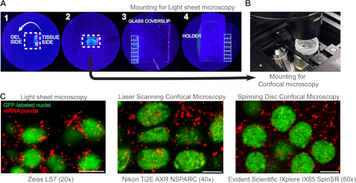
Figure 2. Mounting and imaging expanded samples using light-sheet and confocal microscopy platforms. (A) Visualization and trimming of expanded hydrogels (1–2), common to all imaging platforms, followed by mounting for light-sheet microscopy (3–4; Zeiss Lightsheet 7). (B) Photograph of an expanded sample mounted on an inverted laser-scanning confocal microscope (Nikon Ti2-E AXR). (C) Representative single optical sections (single Z planes) of an expanded Drosophila visual system sample (LC4 neurons labeled with a fluorescent nuclear marker) probed for shakB mRNA (see Figure 4), acquired across three imaging platforms. Scale bars, 10 µm (post-expansion tissue). Please click here to view a larger version of this figure.

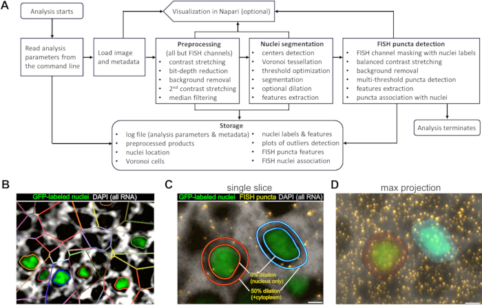
Figure 3. Quantitative analysis of smFISH puncta using FlySeg. (A) Schematic overview of the FlySeg analysis workflow for automated segmentation and puncta quantification within identified cells. (B) Three-dimensional Voronoi tessellation illustrating the core segmentation logic of FlySeg. The imaging volume is partitioned into spatial domains (each shown in a distinct color), with each partition constrained to contain at most one nucleus, ensuring single-cell assignment. Within each Voronoi domain, the nucleus is segmented using a functional optimization procedure that determines the optimal nuclear surface based on both nuclear and surrounding cytoplasmic intensity values. (C) Demonstration of the --nuclei_dilation option to distinguish nuclear and cytoplasmic transcripts A single optical section showing a GFP-labeled nucleus surrounded by smFISH puncta, with diffuse DAPI signal outlining the cytoplasmic compartment following DNase treatment. Lines indicate 0 and 0.5 dilation factors, corresponding to nuclear and cytoplasmic volumes, respectively. (D) Maximum intensity projection of (C), illustrating that puncta localizes both nuclear and cytoplasmic compartments. Scale bars, 10 µm (post-expansion tissue). Please click here to view a larger version of this figure.

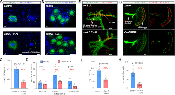
Figure 4. Validation of the quantitative workflow using RNAi-mediated molecular perturbation (A) Light-sheet projections (10 µm thickness, not covering the full cell volume) of the Giant Fiber (GF) soma labeled with a membrane marker and probed for shakB mRNA in control (top) and shakB RNAi (bottom) conditions. Dashed green outlines indicate soma borders to highlight depletion of the cytoplasmic but not nuclear mRNA pool. n, brains (one side per animal). (B) same as (A) for LC4 neurons labeled with a nuclear marker. (C) Quantification of shakB FISH puncta in GF neurons (combined nuclear and cytoplasmic pools) under control and shakB RNAi conditions. Dots represent individual neurons (one neuron per brain, one side per animal). (D) Same as (C) for LC4 neurons. Dots represent individual brains (one side per animal; puncta count per cell averaged per brain). (E) Confocal projections of the GF dendrites labeled with a membrane marker and stained for ShakB in control (top) and shakB RNAi (bottom) conditions. (F) Quantification of ShakB protein levels in the GF dendrites measured as mean fluorescence intensity under control and GF>shakB RNAi conditions. n, brains (one side per animal). (G) Confocal projections of LC4 neurons labeled with a membrane marker and expressing smGdP-10xV5-tagged ShakB in control (top) and shakB RNAi conditions (bottom). Dashed green outlines indicate areas of LC4 dendrites and axon terminals on which ShakB-V5 density was assessed (H) Quantification of ShakB-smGdP-V5 protein levels in the LC4 dendrites and axon terminals measured as mean fluorescence intensity under control and LC4 > shakB RNAi conditions. n, brains (one side per animal). Error bars indicate mean ± SEM. All statistical comparisons were performed using two-sided Welch’s t-tests. Scale bars, 10 µm in all images (post-expansion tissue). Please click here to view a larger version of this figure.

Discussion

This protocol combines expansion-assisted HCR-smFISH, pre-expansion immunohistochemistry, and segmentation-based transcript quantification to enable matched RNA and protein measurements in the same genetically defined neurons. By integrating these components into a single workflow, this method should facilitate quantitative, cell-type-specific molecular analysis in the intact Drosophila brain.

Several practical modifications introduced here represent critical steps for combining immunohistochemistry with expansion-assisted HCR-smFISH in the Drosophila brain²⁴. First, immunohistochemistry should be performed prior to tissue expansion and smFISH. Because the protocol includes a Proteinase K digestion step, performing immunohistochemistry after expansion can reduce epitope integrity. Importantly, pre-expansion antibody incubation (24 h primary + 24 h secondary) does not noticeably reduce RNA signal intensity when RNase-clean technique and covalent RNA anchoring are used. Second, primary and secondary antibody concentrations should be increased, typically 2–3× relative to standard whole-mount IHC, to compensate for signal loss associated with Proteinase K digestion and tissue expansion. Third, fixation conditions are important for preserving both protein and RNA signal. Acid-free glyoxal fixation enhances preservation of punctate synaptic protein localization, maintains structural integrity of neuronal processes, and does not compromise quantitative detection of mRNA puncta. We also observed that simultaneous anchoring of RNA and protein is compatible with both downstream HCR-smFISH and immunofluorescence detection. Together, these adjustments improve compatibility between immunohistochemistry and expansion-assisted transcript detection.

Expansion adds a single overnight step and is not technically complex, but its use depends on the experimental goal. As demonstrated in Supplemental Figure 1, non-expanded FISH combined with immunohistochemistry is sufficient to assess whether a gene is expressed in a given cell type, whereas expansion is required when individual smFISH puncta need to be reliably resolved, assigned to individual somata, and quantitatively analyzed, due to the substantial increase in effective spatial resolution. Similarly, Terasaki-style multiwell plates are not strictly required, but they reduce reagent use, allow multiple conditions to be processed in parallel, and help maintain sample identity across small batches; standard microcentrifuge tubes can also be used when reagent volume is less limiting. Although light-sheet microscopy enables rapid volumetric imaging of expanded tissue, we demonstrate that standard inverted laser-scanning and spinning disk confocal systems are sufficient for complete imaging of the select neuronal populations in the expanded Drosophila brain. A common limitation of confocal microscopy is short working distance. However, because the fly brain is small and samples are expanded approximately 2× in PBS, long-working-distance water-immersion objectives provide adequate penetration depth. For quantitative comparisons, acquisition settings should be kept identical across samples, saturated pixels should be avoided, and voxel size should be sufficient to resolve individual smFISH puncta. This expands accessibility of the protocol to laboratories without dedicated light-sheet instrumentation.

The updated FlySeg implementation builds on the previously published FlySeg framework and introduces two main additions for this protocol. First, a configurable nuclear dilation parameter allows smFISH puncta to be classified as nuclear or cytoplasmic based on their spatial relationship to segmented nuclei. Cytoplasmic DAPI staining after DNase treatment is important for this step, as it provides a diffuse signal outlining the cell body and supports reliable nuclear segmentation, supporting separation of nuclear and cytoplasmic transcript pools. Second, automated outlier detection identifies poorly segmented nuclei, which can be excluded from downstream quantification. Beyond assessing the molecular effects of cell-type-specific gene knockdown, separating nuclear and cytoplasmic transcripts can be informative when transcript localization reflects ongoing transcriptional activity. In the mammalian brain, activity-induced immediate early gene transcripts appear first in the nucleus and subsequently accumulate in the cytoplasm as mRNAs are processed and exported³⁹, a principle used in catFISH⁴⁰ analysis of neuronal activation times. Whether comparable transcriptional dynamics occur in the Drosophila brain is currently unknown, but this can in principle be explored using the present workflow. In any other pulse-chase experiments, distinguishing nuclear from cytoplasmic puncta may therefore provide temporal information beyond total transcript counts. At the same time, the workflow is not restricted to nuclear segmentation and can be adapted to whole-soma (i.e., membrane-defined) cell segmentation. The current quantitative workflow is optimized for neuronal somata; although neuropil regions can be imaged, quantitative assignment of mRNA puncta to individual axons or dendrites would require additional compartment-specific segmentation strategies. FlySeg is most useful for automated, high-throughput quantification in dense neuronal populations where population-level statistics are required. For individually identifiable neurons or manually defined compartments, other tools such as Imaris or FIJI/ImageJ may be more appropriate. A summary of these quantification strategies, including their main applications, advantages, and limitations, is provided in Supplemental Table 1.

Common troubleshooting points include weak antibody signal, high smFISH background, gel damage or sample loss, sample drift during imaging, and poor segmentation. Weak antibody signal can often be improved by further increasing antibody concentration or extending primary and/or secondary antibody incubations from 24 h to 48 h. High smFISH background can often be reduced by extending post-hybridization washes and avoiding saturated acquisition settings. Gel damage and sample loss are minimized by using wide-bore tips, trimming gels with straight cuts, and cutting vent channels to prevent bubbles during chamber filling. Sample drift during imaging is reduced by equilibrating mounted gels for at least 1 h before acquisition; if drift persists, equilibration can be extended to 2 h or longer. Poor segmentation can result from weak cytoplasmic DAPI staining or incomplete sample equilibration, which can reduce cell-boundary signal or cause X-Y-Z shifts during acquisition; these should be checked before adjusting FlySeg parameters. In this protocol, gels are maintained in 1× PBS, resulting in approximately 2× isotropic expansion. If higher spatial resolution is required, greater expansion can be achieved in diluted PBS or deionized water. Conversely, when the goal is only to assess presence or absence of expression in a defined cell type, non-expanded FISH combined with immunohistochemistry may be sufficient, as demonstrated in Supplemental Figure 1. The protocol remains compatible with iterative FISH workflows. Probes and HCR hairpins can be removed by DNase treatment, allowing additional rounds of hybridization and amplification in the same specimen. Future technical extensions could include higher-plex iterative HCR-smFISH, automated registration across imaging rounds, improved whole-cell or neurite segmentation, and more standardized analysis pipelines for comparing RNA and protein signals across experiments. Further development of compartment-specific segmentation strategies could extend quantitative analysis beyond neuronal somata to axons and dendrites. Together, the combined RNA–protein readout, compartment-resolved transcript quantification, and compatibility with standard imaging platforms make this workflow suitable for targeted molecular validation experiments in genetically defined neurons of the intact Drosophila brain.

Materials

List of materials used in this article

Name	Company	Catalog Number	Comments
10N Sodium Hydroxide Solution	Fisher Scientific	Cat# SS255-1
1N Sodium Hydroxide Solution	Fisher Scientific	Cat# SS266-1
20X Saline-Sodium Citrate Buffer	Invitrogen	Cat# AM9763
4-Hydroxy-TEMPO	Sigma-Aldrich	Cat# 176141
5M Sodium Chloride Solution	Sigma-Aldrich	Cat# S5150
Acrylamide	Sigma-Aldrich	Cat# A9099
Acrylic acid	Sigma-Aldrich	Cat# 147230
Acryloyl-X, SE	Invitrogen	Cat# A20770
Adobe Illustrator	Adobe	N/A
Alexa Fluor 488 Goat Anti-Chicken (1:200)	Jackson ImmunoResearch Labs	Cat# 103-545-155, RRID:AB_2337390
Alexa Fluor 568 Goat Anti-Mouse IgG1 (1:200)	Invitrogen	Cat# A-21124, RRID:AB_2535766
Alexa Fluor 568 Goat Anti-Rabbit IgG1 (1:200)	Invitrogen	Cat# A-11011, RRID:AB_143157
Ammonium persulfate	Sigma-Aldrich	Cat# A3678
Anhydrous DMSO	Sigma-Aldrich	Cat# 900645-4X2ML
Bondic UV-curing adhesive	Bondic	Bondic starter kit
cellSens imaging software v4.4.1	Evident Scientific	N/A
Chicken Polyclonal Anti-GFP (1:400)	Abcam	Cat# ab13970, RRID:AB_300798
Conda (environment manager)	Anaconda, Inc	N/A
Corning™ Frosted Microscope Slides	Corning	Cat# 2948-75X25
Custom Designed LS7 Sample Holder	Janelia Tech	ID 2021-021
DAPI	Sigma-Aldrich	Cat# D9542
Disposable Stainless Sterile Scalpel	MedPride	MPR-47101
Ethylenediaminetetraacetic acid	Sigma-Aldrich	Cat# EDS-100G
Fiji (ImageJ) image analysis software v2.14.0	ImageJ Consortium	N/A
FlySeg (custom pipeline)	https://github.com/avaccari/DrosophilaFISH	N/A
GAF fixative solution	Addax Biosciences	Cat# VI25
GenClone® 24 Well Cell Culture Plates, Non-treated	Genesee Scientific	Cat# 25-102
GMR-86D05-Gal4 (LC4)	Bloomington Stock Center	#41315
Goat Serum Donor Herd	Sigma-Aldrich	Cat# G6767
HCR™ RNA-FISH(v3.0) Amplifier Buffer	Molecular Instruments	N/A
HCR™ RNA-FISH(v3.0) Amplifiers:AF546, JF669	Molecular Instruments	N/A
HCR™ RNA-FISH(v3.0) Probe Hybridization Buffer	Molecular Instruments	N/A
HCR™ RNA-FISH(v3.0) Probe Wash Buffer	Molecular Instruments	N/A
HCR™ RNA-FISH(v3.0) ShakB Probe	Molecular Instruments	N/A
Imaris 10.1	Oxford Instruments	N/A
IXPlore IX85 SpinSR Spinning Disk Confocal Microscope	Evident Scientific	N/A
LS7 Light Sheet Microscope	Carl Zeiss	N/A
Melphalan	Cayman Chemical	Cat# 16665
MOPS Buffer	Fisher Scientific	Cat# BP308-100
Mouse Monoclonal Anti-V5 (SV5-Pk1) (1:100)	Abcam	Cat# ab27671, RRID:AB_471093
N,N,N’,N’-Tetramethylethylenediamine	Sigma-Aldrich	Cat# T7024
N,N’-Methylenebisacrylamide	Sigma-Aldrich	Cat# M7279
Napari	open-source community	N/A
NIS-Elements Advanced Research imaging software	Nikon Corporation	N/A
Nuclease-Free Water	Qiagen	Cat# 129114
Nunc™ MiniTrays with Nunclon™ Delta surface	Invitrogen	Cat# 163118
PBS (10X), pH 7.4	Gibco	Cat# 70011044
Photo-Flo detergent	Electron Microscopy Sciences	Cat# 74257
Poly-L-Lysine solution	Ted Pella	Cat# 18026
Precision Cover Glasses, #1.5H Thickness	Thorlabs	Cat# CG15CH2
Press-to-Seal™ Silicone Isolator with Adhesive, one well, 20 mm diameter, 0.5 mm deep	Invitrogen	Cat# P24740
Proteinase K	New England  Biolabs	Cat# P8107S
Rabbit Anti-ShakB (1:400)	Gift from Geord Ammer	N/A
RNase AWAY™ Surface Decontaminant	Invitrogen	Cat# 7002
RNase-Free DNase Set	Qiagen	Cat# 79256
Schneider’s Drosophila Medium	Gibco	Cat# 21720001
shakB-KDRT-stop-KDRT-smGdP-V5;;	Frighetto et al., 2025	PMID: 41278920
Sodium azide	Sigma-Aldrich	Cat# S8032
Stemi 508 Stereo Microscope	Carl Zeiss	N/A
SYTO™ 41 Blue Fluorescent Nucleic Acid Stain	Invitrogen	Cat# S11352
Ti2E AXR NSPARC Laser Scanning Confocal Microscope	Nikon Corporation	N/A
Tris Base	Fisher Scientific	Cat# BP152-500
Triton™ X-100	Sigma-Aldrich	Cat# T8787
UAS-GFP-2A-KDR;	Sanfilippo et al. 2024	PMID: 38262414
UAS-his2A-GFP;	Dombrovski et al., 2025	PMID: 40468081
UAS-mCherry RNAi	Bloomington Stock Center	#35785
UAS-myr::GFP;	Bloomington Stock Center	#32198
UAS-shakB RNAI	Ammer et al., 2022	PMID: 35385694
UltraPure™ 1M Tris-HCI, pH 8.0	Invitrogen	Cat# 15568025
VT042336-Gal4 (Giant Fiber)	Dombrovski et al., 2025	PMID: 40468081
Zen Black 3.1	Carl Zeiss	N/A