Mapping Microglial Parameters Software (MMPS): An Open-Source, User-Friendly Tool for Quantitative Microglia Morphology Analysis

Summary

Mapping Microglial Parameters Software (MMPS) is a user-friendly analysis pipeline that requires no coding expertise and semi-automates single-cell microglial morphology analysis from immunofluorescence images. Validated in a rodent lipopolysaccharide-induced neuroinflammation model, MMPS reproducibly detects activation-associated morphological changes and enables standardized, scalable microglial phenotyping.

Abstract

Microglia are myeloid-derived immune cells of the central nervous system that mediate tissue degradation and remodeling following neurological injury and have emerged as promising therapeutic targets in several neurodegenerative diseases. Quantitative analysis of microglial morphology can reveal subtle differences among microglial subpopulations while preserving important in situ information. However, many currently available microglial morphology analysis platforms are either not publicly accessible or require specialized computational expertise, thereby limiting their widespread adoption. To address these limitations, an open-source microglial morphology analysis platform, termed Mapping Microglial Parameters Software (MMPS), using Python 3.11 was developed. MMPS is compatible with immunofluorescence-based workflows and requires no coding expertise for installation or operation. The software semi-automates single-cell microglial morphology analysis through an accessible graphical user interface and incorporates customizable image-processing and mask-generation workflows. The study involves validating MMPS using a rodent lipopolysaccharide (LPS)-induced neuroinflammation model. Quantitative animal-level analysis demonstrated that microglia from LPS-treated animals exhibited significantly increased soma area (p < 0.01) and reduced cell perimeter (p < 0.05) compared with vehicle-treated controls, consistent with morphological features associated with microglial activation and neuroinflammation. Overall, MMPS provides a standardized, reproducible platform for quantitative analysis of microglial morphology across laboratories.

Introduction

Microglia are innate immune cells of the central nervous system (CNS) that continuously survey their surroundings for pathogens and tissue damage¹. Upon activation, microglia retract their processes and transition from a homeostatic, ramified morphology to an amoeboid phenotype^2,3. In neurodegenerative diseases such as ischemic stroke^4,5 and Alzheimer’s disease^6,7. Microglia often perpetuate neuroinflammation through sustained cytokine production, extensive tissue degradation, and phagocytosis². These processes contribute to disruption of the neurovascular unit, further exacerbating microglial activation and CNS injury⁸, thereby making microglia promising therapeutic targets^9,10.

One approach for identifying subtle differences among microglial subpopulations in neurodegenerative diseases is through morphological analysis. This is commonly performed using Cx3CR1-GFP animals with in vivo two-photon microscopy¹¹ or through immunofluorescence (IF) labeling of established microglial markers such as ionized calcium-binding adaptor molecule-1 (Iba1) or P2Y purinoceptor receptor¹². Although microglia frequently transition between homeostatic and amoeboid morphologies following injury, previous studies have demonstrated that microglia can also adopt additional phenotypes, including hyper-ramified microglia^3,13, honeycomb microglia^3,14, reactive microglia¹⁵, and rod microglia^3,16. However, microglial morphology studies often rely on manual categorization of homeostatic and amoeboid phenotypes. These approaches require specialized analysis pipelines that frequently lack standardization between laboratories and make differentiation between similar morphologies, such as homeostatic versus hyper-ramified phenotypes, difficult even for trained personnel¹⁷. Furthermore, IF-based analysis of subtle morphological alterations requires high-resolution imaging, which can present additional technical challenges.

To address these limitations, several analytical platforms have been developed that semi-automatically¹¹ or automatically¹⁸ detect microglia and generate multiple binary representations of the cells, referred to as “masks,” across user-defined target areas (e.g., 200–800 µm²). These approaches reduce user bias, improve reproducibility, and increase analytical efficiency. Despite these advances, many currently available software platforms have limitations that restrict widespread adoption, including a lack of open-source accessibility¹⁷, requirements for coding expertise^11,19,20, dependence on in vivo two-photon microscopy systems^11,19, absence of intuitive graphical user interfaces^11,21,22, slow processing speeds¹¹, or reliance on commercial software platforms^12,19,21. Although recent studies have begun to address several of these issues, many existing platforms remain poorly suited for IF-based workflows, which remain widely used for studying microglial morphology.

Presented here is a user-oriented microglial morphology analysis platform termed Mapping Microglial Parameters Software (MMPS). MMPS requires no coding expertise, integrates with established ImageJ-based workflows, and is designed specifically for use with IF images. The software was developed in Python 3.11 and incorporates concepts from previously published open-source morphology platforms¹¹. MMPS features an intuitive graphical user interface that enables users to import and process large batches of IF images using multiple customizable image-processing options. The platform also incorporates manual cell selection to minimize oversampling artifacts introduced during IF imaging, as well as manual soma outlining to prevent the inclusion of cellular processes in soma measurements. In addition, MMPS includes customizable mask-generation parameters and multiple quality-assurance features to improve mask accuracy. The software calculates several commonly used morphological parameters, including perimeter, average centroid distance, mask area, eccentricity, roundness, and soma area. For more advanced studies, MMPS-generated outputs are compatible with multiple ImageJ plugins and can be further analyzed using accompanying plugins for fractal, skeleton, and hull analyses.

MMPS was validated using a rodent lipopolysaccharide (LPS)-induced neuroinflammation model by examining microglial alterations within cortical layer IV. Quantitative analysis demonstrated that LPS administration significantly increased microglial soma area while decreasing cell perimeter compared with vehicle-treated controls, indicating that MMPS accurately detects subtle morphological changes associated with microglial activation.

Protocol

All animal procedures were performed in accordance with the West Virginia University Institutional Animal Care and Use Committee (protocol #2109047180) and the Guide for the Care and Use of Laboratory Animals supported by the National Institutes of Health. The equipment, reagents, and software used in this method are listed in the Table of Materials.

1. Experimental animals

1. Procure 10 male Sprague-Dawley rats (2-3 months old). Once rats arrive at the animal facility, they should be group-housed under a 12 h light/dark cycle with ad libitum access to food and water. Upon arrival, rats are acclimated for 3 days before use.
2. Randomly assign rats to vehicle or LPS-treated groups (n = 5 rats/group).
   NOTE: Due to the small number of rats to be used, a simple randomization strategy can be employed, with computer-generated random numbers to assign the rats to a treatment group.
3. Monitor rats following treatment for “sickness behavior”: weight loss (>15%), porphyrin secretion, respiratory abnormalities, or reduced activity.
   NOTE: Sickness behavior symptoms often occur within the first 12 h after administration, so inject agents early in the morning (6-8 AM), monitor behavior throughout the day, and return rats to the facility late in the day (5-7 PM).

2. Neuroinflammation model

1. Prepare LPS (O111:B4) stock solution (10 mg/mL) by dissolving 50 mg LPS in 5 mL phosphate-buffered saline.
   NOTE: LPS is an endotoxin. Researchers should follow their institution’s SOP for handling and disposal.
2. Weigh rats and then inject intraperitoneally with LPS (10 mg/kg) or PBS (vehicle).
3. Based on the weight of the rats, an injection volume between 150–300 µL is expected.
4. Euthanize rats 24 h after injection by cardiac perfusion followed by decapitation.
5. Anesthetize rats with inhaled isoflurane (5% in O₂) for 5–10 min. Confirm anesthesia by the absence of the pedal withdrawal reflex.
6. While anesthetized, create a midline thoracic incision to expose the diaphragm and sternum. Clamp the xiphoid process using hemostats to reveal the thoracic cavity.
7. Cut the diaphragm and rib cage toward the forelimbs to expose the heart.
8. Clamp the descending aorta and inferior vena cava with hemostats. Insert a 25-gauge winged needle into the left ventricle.
9. Perfuse rats with ice-cold PBS (25 mL at 30 mL/min) using a peristaltic pump. Incise the left atrium within several seconds of initiating perfusion to allow perfusate drainage.
10. Perfuse rats with 4% paraformaldehyde (25 mL at 30 mL/min).
    CAUTION: Handle paraformaldehyde using appropriate personal protective equipment in a well-ventilated environment. Dispose of paraformaldehyde waste according to institutional and local regulations.
11. Decapitate rats with a guillotine following perfusion.
    NOTE: Follow your institution’s guidelines regarding logging of decapitations and sharpening of blades.
12. Expose the skull by retracting the scalp toward the pinna.
13. Break the frontal bone using hemostats or rongeurs inserted into the orbital sockets.
14. Insert forceps into the foramen magnum and peel away the parietal bones.
15. Remove the brain using fine forceps and incubate overnight in 4% paraformaldehyde.
16. Transfer brains sequentially into 20% sucrose and 30% sucrose overnight for cryoprotection.

3. Immunofluorescence

1. Freeze cryoprotected brains in Tissue Tek O.C.T. Compound on dry ice.
2. Section brains at 30 µm using a cryostat.
3. Collect sections in PBS and transfer them into net wells inserted into a 12-well plate.
4. Select at least two sections per rat containing the anterior dorsal hippocampus.
5. Wash sections in PBS for 5 min twice while rocking.
6. Permeabilize sections in 0.3% Triton X-100/PBS for 45 min while rocking.
   NOTE: Use 3 mL solution per wash or incubation step unless otherwise specified.
7. Wash sections in PBS for 5 min twice.
8. Dilute the antigen retrieval solution to 1x in PBS and add 2 mL per well.
9. Incubate sections at 80°C for 20 min using a water bath.
10. Allow sections to cool to room temperature before proceeding.
11. Wash sections in PBS for 5 min twice.
12. Block sections in 10% donkey serum/0.05% Triton X-100/PBS for 2 h at 37°C while shaking at 75 rpm.
13. Wash sections in 1% donkey serum/0.05% Triton X-100/PBS for 5 min three times.
14. Transfer sections into a new 12-well plate without the net wells containing 500 µL of primary anti-Iba1 antibody solution prepared in 1% donkey serum/0.05% Triton X-100/PBS.
15. Prepare negative controls by omitting the primary antibody from the incubation solution.
16. Incubate all sections overnight at 4°C on an orbital rocker
17. Return sections to net wells.
18. Wash sections in 1% donkey serum/0.05% Triton X-100/PBS for 10 min three times.
19. Incubate sections with anti-rabbit secondary antibody (1:1000 dilution) in 1% donkey serum/0.05% Triton X-100/PBS for 1.5 h at room temperature.
    NOTE: Minimize light exposure during all subsequent procedures and wrap plates in aluminum foil to prevent fluorophore degradation.
20. Wash sections in PBS for 5 min twice.
21. Mount sections onto microscope slides.
22. Air-dry slides in darkness for >2 h.
23. Coverslip sections using water-soluble compounds.
24. Prepare negative-control slides using a mounting medium.
25. Store slides in a slide box at room temperature in a dark environment.

4. Imaging

1. Identify the pixel size of an imaging system at 40x magnification. If the scale is not found, add a scale bar to each image.
2. Use DAPI staining to identify a dense band of cortical nuclei at low magnification corresponding to cortical layer IV.
3. Focus the image on the identified cortical region.
4. Switch to the 40x magnification .
5. Adjust channel exposure settings to maximize separation of DAPI and Iba1 signal from background fluorescence.
6. Acquire Z-stack images (> 30 steps) spanning the full depth of the microglia.
7. Generate and save a composite maximum-intensity projection image from the acquired Z-stack of both stains.
   NOTE: Optimize exposure and Z-stack settings for each image to maximize signal separation between DAPI/Iba1 and background fluorescence. Poor signal separation reduces mask-generation accuracy.

5. Mapping microglial parameters software (MMPS)

1. Store all composite images in a single image directory.
2. Create a separate output directory for MMPS-generated results.
3. Download the MMPS standalone package or MMPS.py script from the GitHub repository.
4. Install all dependencies listed in the requirements.txt file if launching MMPS through MMPS.py.
5. Open MMPS package or run MMPS.py script.
6. Select “Select the Image Folder” and choose the image directory.
7. Select “Select Output Folder” and choose the output directory.
8. Grant folder-access permissions if prompted by the operating system.
   NOTE: Additional installation instructions, troubleshooting guidance, and usage examples are provided in the supplementary documentation and GitHub repository.
9. Select “Image Labeling” and assign animal identifiers and treatment groups to each image.
   NOTE: If image labeling is skipped, MMPS prompts for treatment-group and animal identifiers before data export.
10. Enter the pixel size under the “Parameters” tab.
11. Select “Calibrate from scale bar” if the pixel size is unknown. Select the beginning and end points of the scale bar when prompted. Enter the known scale-bar distance in micrometers.
12. Select the fluorescence channel containing the microglial signal.
13. Select images for processing by checking the box next to each image name. Process images individually when background fluorescence differs substantially between images.
14. Review the “Original,” “Preview,” “Processed,” and “Masks” tabs to compare image-processing stages.
15. Select “Preview Current Image” to evaluate image-processing settings.
16. Adjust rolling-ball background subtraction, denoising, and sharpening settings as needed.
17. Use rolling-ball values between 5–150 pixels for background subtraction.
18. Use denoising values between 3–7 pixels to reduce uneven illumination artifacts.
19. Use sharpening values between 1–2 to improve edge definition.
20. Select “Process Selected Images” after optimization of image-processing settings.
    NOTE: Image-processing time varies depending on image number and selected parameters.
21. Select “Pick Somas (All Images).”
22. Select “Show Color (C)” to display RGB composite images. Select “Channels…” and deselect unused channels if image coloration appears distorted.
23. Select microglial somas displaying DAPI and Iba1 colocalization. Avoid selecting cells contacting image borders. Remove incorrectly selected soma markers using the “Backspace” or “Delete” key.
24. Press “Enter” or “Return” to proceed to the next image.
25. Select “Outline Somas (All)” after soma selection is complete.
26. Outline the soma perimeter of each selected microglial cell. Exclude cellular processes from the soma outline and use at least eight outline points per soma. Remove incorrectly placed outline points using “Undo Last Point,” “Delete,” or “Backspace.”
27. Press “Enter,” “Return,” double-click, or right-click to finalize each soma outline.
28. Select “Redo Last Outline” to repeat the previous soma outline if needed.
29. Select “Generate All Masks” after completion of soma outlining.
30. Apply a minimum threshold value to restrict the incorporation of low-intensity background pixels into masks.
    NOTE: Higher values preserve soma accuracy at the expense of branching, while lower values preserve branching accuracy at the cost of soma. Threshold values between 10–30% typically provide balanced background suppression and branch preservation.
    NOTE: Mask generation time varies depending on the number of selected cells.
31. Select “QA All Masks” to begin mask quality assurance.
32. Review masks presented from largest (800 µm²) to smallest (200 µm²).
33. Compare each mask to the corresponding microglia using the “Processed” and “Mask” tabs.
34. Accept masks using the “A” keyboard shortcut. Reject masks using the “R” keyboard shortcut. Press “B” to undo an acceptance or rejection. Navigate through mask sizes using the keyboard arrow keys.
35. Select the largest acceptable mask that accurately captures microglial branching without including neighboring cells, excessive background, image borders, or scale bars.
    NOTE: Reject masks if there is uncertainty about their accuracy.
    NOTE: Select “Clear All Masks,” then regenerate the masks with a different threshold value if most are inaccurate.
36. Select “Calculate Simple Characteristics” after mask quality assurance is complete to
    calculate average centroid distance, mask area, perimeter, eccentricity, roundness, and soma size using accepted masks and soma outlines.
37. Refer to Table 1 for parameter definitions and microglial trends in neuroinflammation.
38. Download “Sholl.py,” “FractalAnalysis_ImageJ.py,” and “SkeletonAnalysisImageJ.py” to perform additional analyses.
39. Open “FractalAnalysis_ImageJ.py” as a Fiji plugin for fractal and hull analyses.
40. Enter the output-directory location and pixel size when prompted. Select the “largest mask only” option if analysis of only the largest accepted mask is desired.
41. Open “Sholl.py” as a Fiji plugin for Sholl analysis.
42. Enter the output-directory location and pixel size when prompted.
43. Enter the desired Sholl-analysis step size. Select “Use soma radius as start radius” to use MMPS-derived soma radii as the starting radius for Sholl analysis. Enter a fixed soma radius value if MMPS-derived soma radii are not used.
44. Open “SkeletonAnalysisImageJ.py” as a Fiji plugin for skeleton analysis.
45. Enter the output-directory location, pixel size, and masks-folder location when prompted.
46. Export all plugin-generated results as CSV files into the output directory when finished.

6. Formulas used in MMPS for microglia morphology calculations

NOTE: All calculations are performed automatically by MMPS when “Calculate Simple Characteristics” is pressed. Parameter calculations are shown below.

1. Perimeter
   1. Calculate perimeter using the following equation:
      
   2. Define as perimeter, as the number of edge pixels, and as pixel size in µm.
2. Average centroid distance
   NOTE: Average centroid distance is also referred to as cell spread¹¹.
   1. Identify four branch endpoints based on cell coordinates:
      top branch: minimum y-coordinate,
      bottom branch: maximum y-coordinate,
      left branch: minimum x-coordinate,
      ​right branch: maximum x-coordinate.
   2. Calculate the centroid coordinates using the following equations:
      
      
   3. Define c_x and c_y as centroid coordinates, x_i and y_i as pixel coordinates, and as the total number of pixels.
   4. Calculate branch distance using the following equation:
      
   5. Define d as branch distance, x_i and y_i as branch-end coordinates, and c_x and c_y as centroid coordinates.
   6. Calculate average centroid distance using the following equation:
      
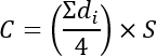
   7. Define as the average centroid distance, as branch distance, d_i and as pixel size in µm.
3. Mask area
   1. Calculate mask area using the following equation:
      
   2. Define as mask area in µm², as the number of pixels within the mask, and as pixel size in µm.
4. Eccentricity
   1. Calculate second central moments using the following equations:
      
      
      
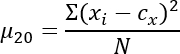
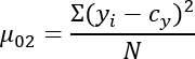
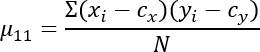
   2. Define μ₂₀, μ₀₂, and μ₁₁ as second central moments, x_i and y_i as pixel coordinates, c_x and c_y as centroid coordinates, and N as the total number of pixels.
   3. Calculate covariance-matrix eigenvalues using the following equation:
      
   4. Define λ₁ ≥ λ₂.
   5. Calculate major and minor axis lengths using the following equations:
      
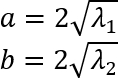
   6. Define a as major axis length and b as minor axis length.
   7. Calculate eccentricity using the following equation:
      
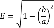
   8. Define as eccentricity.
5. Roundness
   1. Calculate roundness using the following equation:
      
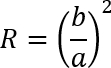
   2. Define as roundness, as major axis length, and as minor axis length.
6. Soma size
   1. Calculate soma area using the following equation:
      
   2. Define Sa as soma area in µm², as the number of pixels within the soma mask, and S as pixel size in µm.

7. Statistical analysis

1. Perform all statistical analyses using R version 4.3.2.
2. Filter datasets using the largest accepted mask for each cell.
3. Average cellular parameters at the animal level before statistical analysis.
4. Assess normality and variance using the Shapiro–Wilk and Levene tests.
5. Perform Student’s t-tests or repeated-means ANOVA with post-hoc Holm-corrected paired t-tests when datasets satisfy parametric assumptions.
6. Perform Wilcoxon rank-sum or Friedman tests with Holm-corrected paired Wilcoxon signed-rank tests when datasets do not satisfy parametric assumptions.
7. Define statistical significance as p < 0.05 .

Results

An open-source, standalone microglial morphology analysis platform, termed Mapping Microglial Parameters Software (MMPS), was developed to provide an accessible, standardized workflow for IF-based microglial morphology analysis. The platform builds on previous morphology-analysis methodologies, requires no coding expertise, and incorporates an accessible graphical user interface. MMPS was designed to improve the detection of subtle microglial branching while incorporating multiple safeguards to minimize the overestimation of microglial masks.

MMPS was validated using an LPS-induced rodent neuroinflammation model. Following tissue processing and image acquisition (Figure 1), IF specificity was confirmed using negative-control sections lacking primary antibody staining (Supplementary Figure 1). MMPS processing begins with the importation of IF images into the software interface (Figure 2A). The software provides multiple image-processing options to improve microglial signal detection and background separation. Mandatory background subtraction is performed using the rolling-ball algorithm implemented in the Scikit-image package, while optional denoising and sharpening filters are available via SciPy-based Gaussian filtering. Following image processing, microglial somas are manually selected and identified by red selection markers (Figure 2B). Soma boundaries are subsequently outlined manually for downstream morphological calculations (Figure 2C).

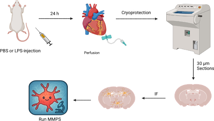
Figure 1: Graphical overview of neuroinflammation model and processing. Rats were injected with LPS or PBS and collected 24 h with a cardiac perfusion followed by decapitation. Brains were extracted and sliced into 30 µm sections to then be used in IF for microglial marker Iba1 which were then processed with MMPS. Created with Biorender. Please click here to view a larger version of this figure.

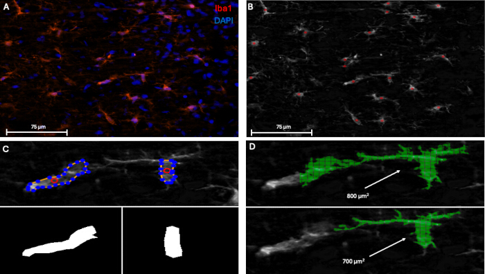
Figure 2: Overview of MMPS usage. (A) Example of an image of cortical microglia (red, Iba1) with cell nuclei (blue, DAPI) to be referenced in MMPS (scale bar = 75 µm, 40x) . After image processing using MMPS, the background will be reduced and accurate morphologies assessed (B) After processing the image in MMPS, somas are manually selected with a red circle to be used in subsequent steps detailed in the methods (scale bar = 75 µm, 40x). (C) Two representative microglia were manually outlined, and the saved soma outline images are shown below. (D) Mask generation of selected cells automatically traces microglial branches up to 800 µm², but it requires manual quality assurance. Here we display the inaccurate 800 µm² mask followed by the more accurate 700 µm² mask. Please click here to view a larger version of this figure.

After soma outlining, MMPS generates masks iteratively across a size range of 200–800 µm² using adaptive thresholding constrained by user-defined minimum-intensity thresholds. Smaller masks more closely follow the user-defined threshold, whereas larger masks progressively relax threshold restrictions to maximize branch incorporation. Generated masks undergo manual quality-assurance review to prevent inclusion of neighboring cells, excessive background incorporation, or truncation by image borders or scale bars. As shown in Figure 2D, the 800 µm² mask for a representative microglial cell extended into a neighboring cell. Rejection of the 800 µm² mask and selection of the 700 µm² mask corrected the segmentation error while preserving accurate delineation of the target microglia.

Following MMPS processing, microglial activation was assessed using the largest accepted mask for each cell, as these masks most accurately captured distal branching while minimizing background incorporation. Calculated morphological parameters are summarized in Table 1 and represented in Figure 3. LPS administration significantly decreased average centroid distance and cell perimeter compared with vehicle-treated controls (p < 0.05; Figure 3A,B), consistent with retraction of microglial processes during activation. No significant differences were observed in mask area, roundness, or eccentricity between treatment groups (Figure 3C–E), despite previous reports associating these parameters with activated microglial phenotypes^3,23. The present study was not statistically powered to detect subtle differences in soma shape or mask area, and microglial subpopulations can adopt heterogeneous inflammatory morphologies that do not uniformly follow these trends³. In contrast, the soma area was significantly increased in LPS-treated animals compared with vehicle controls (p < 0.01; Figure 3F), further supporting activation-associated morphological remodeling²².

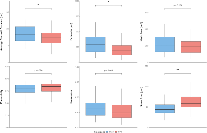
Figure 3: Comparison of microglial morphological parameters. For all panels, tests for normality were conducted (Shapiro-Wilk and Levene) with nonsignificant values found in all cases (p>0.05), leading to Student t-tests being employed. Dots represent individual animals (n=5 per treatment) (A) Average centroid distance was significantly greater in the vehicle group compared to the LPS treatment group. (B) Microglia cell perimeter was significantly greater in the vehicle group compared to the LPS treatment group. (C) There was no significant difference in mask area between treatment groups. (D) There was no significant difference in soma eccentricity between groups. (E) There is no significant difference in soma roundness between treatment groups. (F) There was a significant increase in soma area in the LPS group * p<0.05, ** p<0.01, *** p<0.001. Please click here to view a larger version of this figure.

Parameter	Definition	Relation to Microglial Activation
Average Centroid Distance	Average distance of the furthest branch in the top, right, bottom, and left positions	Decreases
Perimeter	Measurement of the perimeter of the cell	Decreases
Mask Area	The actual area of the cell, not the target mask area	Decreases
Eccentricity	A measurement of the approximate elongation of the cell soma (0: circular, 1: highly elongated)	Decreases
Roundness	A measurement of the approximate circularity of the cell soma (0: elongated, 1: circular)	Increases
Soma Size	The area of the cell soma	Increases

Table 1: Calculated Parameters from MMPS and Predicted Change in Response to Microglia Activation. The table summarizes morphological parameters calculated by Mapping Microglial Parameters Software (MMPS), including perimeter, average centroid distance, mask area, eccentricity, roundness, and soma area.

Inter-user reproducibility was subsequently evaluated by providing the same image set to blinded, previously untrained users for independent analysis (Supplementary Figure 2). No statistically significant differences were detected between users, and all users reproduced morphological trends consistent with microglial activation in LPS-treated animals.

MMPS additionally supports downstream advanced morphological analyses. Correlative analysis of parameters generated from Figure 3 demonstrated relationships between distinct morphological features. Vehicle-treated rats demonstrated only a weak correlation between microglia roundness and perimeter (R² = 0.17), whereas LPS-treated rats demonstrated a stronger correlation (R² = 0.64), suggesting that increased microglial activation was associated with simultaneous reductions in roundness and perimeter (Figure 4A). In addition, the mask area demonstrated strong positive correlations with average centroid distance in both vehicle and LPS-treated groups (R² = 0.71 and 0.88, respectively), consistent with changes in branching complexity associated with microglial activation status (Figure 4B).

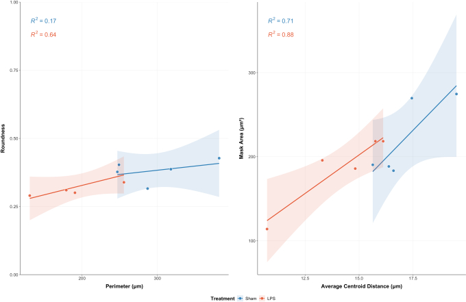
Figure 4: Advanced analysis of microglial parameters. All panels are animal-level lines of best fit computed by the ordinary least squares method displayed with their coefficient of determination (R²) and shaded with their 95% confidence interval. (A) Microglial soma roundness and total perimeter length trend weakly in microglia form the vehicle group (R² = 0.17) but have stronger correlation after LPS exposure (R² = 0.64). (B) Average centroid distance correlates with the area of the microglia in the vehicle (R² = 0.71) and LPS (R² = 0.88) groups. Please click here to view a larger version of this figure.

Supplementary Figure 1: Validation of IF Protocol Through Negative Control. One brain slice of the same region for each rat underwent the IF protocol without primary antibody addition to confirm lack of autofluorescence (scale bar = 75 µm) (A) Representative image of vehicle-stained tissue for DAPI (blue). (B) Representative image of vehicle-stained tissue for Iba1 (red). (C) Representative image of vehicle-stained tissue for DAPI (blue) and Iba1 (red). (D) Representative image of LPS-stained tissue for DAPI (blue). (E) Representative image of LPS-stained tissue for Iba1 (red). (F) Representative image of LPS-stained tissue for DAPI (blue) and Iba1 (red). Please click here to download this file.

Supplementary Figure 2: Assessment of MMPS Inter-User Variation. Several blinded users utilized MMPS on the same samples from Figure 3 and the animal-level results were compared. For all, tests of normality (Shapiro-Wilk and Levene) were nonsignificant (p>0.05), leading to the utilization of a repeated-means ANOVA with post-hoc Holm-corrected paired t-test (p>0.05). (A) There was no significant difference in each group between users for average centroid distance (p>0.05). (B) There was no significant difference in each group between users for perimeter (p>0.05). (C) There was no significant difference in each group between users for mask area (p>0.05). (D) There was no significant difference in each group between users for eccentricity (p>0.05). (E) There was no significant difference in each group between users for roundness (p>0.05). (F) There was no significant difference in each group between users for soma area (p>0.05). Please click here to download this file.

Discussion

The primary goal of this methodology is to expand accessibility to microglial morphology analysis by reducing common technical barriers while preserving the strengths of established morphological assessment approaches. MMPS enables detection of subtle microglial morphological alterations while maintaining compatibility with advanced analyses, including fractal, skeleton, hull, and Sholl analyses. Compared with previously published approaches, MMPS provides an accessible graphical user interface, integrated calculations for commonly used morphological parameters, and elimination of coding requirements while retaining compatibility with more advanced downstream analyses.

Several critical methodological steps strongly influence analytical accuracy and reproducibility. High-quality immunofluorescence (IF) imaging is essential for reliable mask generation and morphology calculations. Antibody specificity represents a major determinant of image quality, as nonspecific labeling increases background fluorescence and reduces signal separation between microglia and surrounding tissue. Similarly, suboptimal antibody concentrations can reduce fluorescence intensity and diminish image resolution. Acquisition of Z-stack images is also critical, as omission of Z-stack imaging can artificially alter apparent microglial branching complexity and process spread, thereby biasing morphological calculations.

Several additional considerations are important during MMPS processing. Although MMPS supports batch image processing, individual image optimization is often preferable because background characteristics and staining quality can vary substantially between images. Image quality directly influences mask generation accuracy; therefore, optimization during image preprocessing substantially improves reproducibility and robustness of downstream analyses. Careful selection of microglial somas is also important, particularly avoidance of cells contacting image borders, as partial-cell selection can artificially reduce soma measurements and distort mask generation. During mask quality-assurance review, masks that incorporate neighboring cells, excessive background, or image borders should be rejected. Conversely, smaller masks should not be rejected solely because they fail to capture all distal processes, as the iterative mask-generation algorithm intentionally adjusts local thresholding parameters according to mask size and regional pixel intensity.

This methodology is highly adaptable and can be modified to meet specific experimental requirements. Because MMPS is open source, the platform can be expanded to analyze individual Z-stack frames or incorporate automated cell-detection algorithms to generate a fully automated morphology-analysis pipeline. In addition, generated masks and soma outlines remain compatible with ImageJ-based workflows for fractal, hull, skeleton, and Sholl analyses. Because MMPS was developed in Python 3.11, additional analyses can also be incorporated directly into the software using commonly available scientific Python packages without requiring external software platforms.

Despite these advantages, several limitations should be considered. MMPS was validated using a neuroinflammation model in a specific brain region of male Sprague-Dawley rats, and different brain regions, disease models, species, or biological sex may influence morphological outcomes. Applicability of MMPS to alternative experimental paradigms should therefore be validated through pilot studies or supported through prior literature comparisons. In addition, IF-based imaging incompletely captures three-dimensional branching structures because processes extending directly above or below the focal plane may not be detected in maximum-projection images. Increasing the number of analyzed cells may help mitigate this limitation. MMPS also remains dependent on image-acquisition quality and therefore requires optimization for individual imaging systems, staining protocols, and antibody preparations. Low-resolution images can artificially inflate mask size because of blurred boundaries surrounding somas and tightly packed branches. For this reason, the present protocol incorporates free-floating IF methods and multiple image-processing options to maximize image quality.

MMPS additionally retains some potential for user-dependent variability because users manually select cells and outline somas. However, use of DAPI and Iba1 colocalization substantially reduces ambiguity during cell selection. Furthermore, blinded inter-user analysis demonstrated minimal variability between previously untrained users, supporting reproducibility of the analytical workflow.

Unlike several previously published microglial morphology platforms, MMPS is not fully automated. However, this design was selected to prioritize segmentation accuracy and mask quality assurance. Automated workflows could be incorporated through modification of the Python source code to enable automated DAPI/Iba1 colocalization detection, contour-based soma outlining, and machine-learning-based mask acceptance or rejection. In addition, MMPS requires substantial disk-storage capacity because generated masks and soma outlines are automatically saved as .tiff files for downstream analyses and quality assurance. Storage requirements could be reduced by modifying the software to generate masks sequentially on a cell-by-cell basis, followed by immediate quality assessment and parameter extraction.

In conclusion, MMPS expands access to quantitative analysis of microglial morphology by providing a standardized, open-source platform that requires no coding expertise or in vivo imaging capabilities. The platform facilitates reproducible analysis of IF-based microglial morphology while maintaining compatibility with advanced downstream analytical approaches.

Materials

List of materials used in this article

Name	Company	Catalog Number	Comments
12-well plate	Fisher Scientific	07-200-82	Plate used for incubation and washing of tissue sections.
Aluminum foil	Fisher Scientific	01-213-101	Used to protect fluorescent samples from light exposure.
Antigen Retrieval Buffer (10×)	ThermoFisher Scientific	00-4955-58	Used to improve antigen accessibility during immunofluorescence staining.
Anti-Iba1 primary antibody	FUJIFILM Wako Pure Chemical Corporation	019-19741	Primary antibody used for immunofluorescent labeling of microglia.
Cryostat	Fisher Scientific	95-710-0L	Instrument used to section frozen brain tissue at defined thicknesses.
Donkey anti-Rabbit IgG, Alexa Fluor 555	ThermoFisher Scientific	A-21428	Fluorescent secondary antibody used for visualization of rabbit primary antibodies.
Donkey Serum	Fisher Scientific	50-413-115	Blocking reagent used to reduce nonspecific antibody binding.
EVOS FL Auto 2 Imaging System	ThermoFisher Scientific	AMAFD2000	Fluorescence microscope used for image acquisition.
Fiji (ImageJ) 2.16.0	NIH	fiji.sc	Image-processing platform used for downstream morphology analyses and plugins.
Fluoromount-G	ThermoFisher Scientific	00-4959-52	Mounting medium used to preserve fluorescence and secure coverslips.
Isoflurane	EntirelyPets Pharmacy	MWI502017	Inhalation anesthetic used during animal procedures.
Lipopolysaccharide	Millipore Sigma	L2630	Used to induce systemic neuroinflammation and microglial activation in rodents.
Matplotlib	https://pypi.org/project/matplotlib/		Python plotting library used for data visualization and figure generation.
MMPS (Mapping Microglial Parameters Software) v1.00	This work	https://github.com/NeurodegenerativePharmaceuticalLab/Mapping-Microglia-Parameters-Software/releases/tag/v1.00	Open-source software platform developed for microglial morphology analysis.
Net wells	Millipore Sigma	CLS3477	Inserts used to hold free-floating tissue sections during staining procedures.
Numpy	https://pypi.org/project/numpy/		Python library used for numerical computations within MMPS.
Objective lens (4×)	ThermoFisher Scientific	AMEP4922	Low-magnification objective used for anatomical orientation and region identification.
Objective lens (40×)	ThermoFisher Scientific	AMEP4625	High-magnification objective used for microglial morphology imaging.
opencv-python	https://pypi.org/project/opencv-python/		Computer vision library used for image-processing functions within MMPS.
Paraformaldehyde	ThermoFisher Scientific	169650025	Fixative used for tissue perfusion and preservation prior to sectioning.
Permount	Fisher Scientific	SP15-100	Permanent mounting medium used for slide preservation.
Phosphate-buffered saline	Fisher Scientific	BP3991	Buffer solution used for tissue washing and reagent preparation.
Pillow	https://pypi.org/project/Pillow/		Python imaging library used for image processing operations.
PyQt5	https://pypi.org/project/PyQt5/		Python GUI framework used to generate the MMPS graphical user interface.
Python 3.11	Python Software Foundation	python.org	Programming language environment used to develop and run MMPS.
R 4.3.2	R Foundation for Statistical Computing	r-project.org	Statistical software used for data analysis and graph generation.
Scikit-image	https://pypi.org/project/scikit-image/		Python image-analysis library used for image processing and segmentation.
Scipy	https://pypi.org/project/scipy/		Python scientific-computing package used for filtering and image-processing operations.
Sprague-Dawley Rats	Evingo	002	Experimental animals used for validation of the neuroinflammation model.
Sucrose	Fisher Scientific	S5-3	Cryoprotectant used prior to freezing brain tissue.
Tifffile	https://pypi.org/project/tifffile/		Python package used for reading and writing TIFF image files.
Tissue-Tek O.C.T. Compound	Sakura Finetek	4583	Embedding medium used for cryosectioning frozen tissue samples.
Triton X-100	Fisher Scientific	BP151-100	Detergent used for membrane permeabilization during immunofluorescence.