Legumes partner with soil bacteria, forming root nodules in which the bacteria fix atmospheric nitrogen for plant use. MicroCT enables non-destructive 3D imaging of the tissue organization, bacteroid zones, and vascular bundles of this opaque hard tissue of the root nodules, providing advantages over traditional imaging techniques that require sectioning nodules.
Method Article
3D MicroCT Imaging of Medicago sativa Root Nodules
* These authors contributed equally
In This Article
Summary
Abstract
The symbiotic relationship between the legume Medicago sativa and the soil bacteria Sinorhizobium meliloti results in the formation of nitrogen-fixing root nodules. Traditional destructive methods, including paraffin sectioning, vibratome sectioning, and cryosectioning, have been applied to visualize how bacteria occupy the nodule, making it extremely difficult to obtain reliable three-dimensional information. These approaches are often combined with fluorescent labeling or staining, which can introduce additional stress affecting plant growth and nodule formation. MicroCT has emerged as a relatively quick, easy, and robust tool for plant biology that can non-destructively visualize plant histological features in three dimensions (3D), thereby avoiding destructive artifacts during sample preparation and ensuring high-fidelity 3D reconstruction. While microCT has been applied to legume root nodules, a detailed established protocol that documents the process from plant harvest and sample preparation to scanning and software visualization is lacking.
In this study, we show a step-by-step microCT workflow using Medicago sativa as a model. The protocol includes nodule excision from roots, fixation, contrast enhancement, mounting, scanning, and three-dimensional reconstruction. Critical parameters affecting elements such as image quality, tissue preservation, and contrast are highlighted. Using this approach, it is possible to visualize the overall tissue organization, bacteroid-infected cells, and vascular bundles in three dimensions without physically sectioning the nodules. The pipeline described here provides a reproducible method for non-destructive, high-resolution imaging of native root nodules and is likely adaptable to other legume species, offering researchers a practical tool for studying nodule structure and bacterial organization within nodules in 3D.
Introduction
Plants in the Leguminosae (or Fabaceae) family such as Medicago sativa (alfalfa) form a symbiotic relationship with nitrogen-fixing soil bacterium in the Rhizobiaceae family like Sinorhizobium meliloti, resulting in the development of root nodules. The plant releases flavonoids to attract the bacteria under nitrogen-limited conditions. This activates the expression of Nod factors in the symbiotic bacteria, triggering root hair curling and subsequent formation of an infection chamber surrounding the bacteria1,2,3,4. An infection thread forms from a weakened section of the chamber wall, creating an elongating tube that carries the bacteria through the root hair cell5. When the infection thread reaches the inner cortex, a series of cell divisions initiates the formation of a specialized root organ called the root nodule1,2,5. The bacteria then infect the nodule cell and live intracellularly, surrounded by the symbiosomal membrane within the cell. Here, the plant provides carbon and other nutrients to the bacteria. In return, the bacteria fix nitrogen for the plant, converting unusable atmospheric nitrogen into ammonia, a plant-useable form2,3,4. Thus, the root nodule functions as a vital biological factory for nitrogen fixation, sustaining plant growth even in the absence of synthetic nitrogen fertilizers. This process of biological nitrogen fixation is economically and environmentally important because it allows legumes to grow in the absence of synthetic fertilizers6. Moreover, some legumes form indeterminate nodules that form distinct zones in which bacteria differentiate and fix nitrogen more efficiently4. Thus, it is important to visualize both the nodule exterior and interior (where the bacteria physically occupy plant cells within the nodule) to study biological nitrogen fixation in detail. However, it is an opaque organ filled with the red-colored plant protein leghemoglobin, which makes traditional imaging methods challenging.
Imaging techniques used in the past have been destructive. Paraffin sectioning, vibratome sectioning, and cryosectioning have been used to produce tissue sections, but these disrupt the native state of the tissue and introduce artifacts that complicate three-dimensional (3D) reconstruction6,7,8,9,10. Reconstruction from paraffin-embedded nodule tissue sections has been successfully completed, but it uses dehydrated samples and requires over 200 individual sections8. In individual sections, portions of the vascular system can be seen, but not how the bundles split and wrap around the nodule. Various fluorescent labeling and staining techniques have been performed on tissue sections prior to confocal microscopy, but these tend to have the following issues8,9,10: (i) Plant nodule tissue is highly autofluorescent, (ii) many methods require tissue clearing prior to imaging, (iii) fluorescent staining can damage nodule tissue, iv) inoculating plants with green fluorescent protein (GFP)-labeled bacteria introduces stress that impacts both plant growth and nodule formation, and v) native nodules are too large to easily section the entire sample5,11.
Commonly employed in medical settings, computed tomography (CT) imaging is used for both diagnostic and therapeutic purposes12,13. A smaller version of this, X-ray microtomography (MicroCT), is an imaging technique that allows for non-destructive three-dimensional (3D) visualization of small subjects. While CT rotates the machine around the larger subject, microCT rotates the smaller subject close to the X-ray source. This allows for much higher resolution. MicroCT has been applied to animal developmental biology, but it has also emerged as a promising tool in plant biology6,10,14,15,16,17,18,19. Importantly, microCT and synchrotron-based X-ray tomography have been used extensively in plant physiology to investigate xylem embolism and to cross-validate imaging-based estimates against conventional hydraulic flow measurements20,21,22. Because it images intact organs at scales without physical sectioning, microCT preserves spatial relationships across the whole nodule. With appropriate contrast agents, it resolves tissue-level structures such as vascular bundles and infection zones, and can penetrate beyond where light scattering limits conventional optical approaches, which is particularly valuable for opaque and auto-fluorescent nodules. Samples can also be rescanned, incorporated into downstream correlative workflows following light or electron microscopy sample processing, or archived for future analysis. Although a few studies have used microCT and synchrotron-based X-ray CT to investigate soybean root nodules, there is no detailed record that covers the full process from nodule harvest and staining through imaging and reconstruction, especially for smaller nodules such as those of alfalfa6,14. X-ray contrast depends on tissue density, and most plant tissue is low-density and poorly X-ray attenuating. Without a contrast agent, nodules cannot be distinguished from the background on a conventional benchtop microCT. We used phosphotungstic acid (PTA), a non-specific stain that binds proteins and other biomolecules and has been shown to produce high contrast in plant tissue14.
This study provides an in-depth, step-by-step protocol for microCT imaging of legume root nodules using alfalfa as a model, on a conventional lab-based system that offers a more accessible alternative to X-ray microscopy (XRM) and synchrotron-based platforms6,14. This workflow features specific instructions for nodule harvest from the root, fixation, staining, contrast enhancement, mounting, scanning, 3D reconstruction, and analysis (Figure 1). Between these steps, we provide detailed parameters to ensure stable mounting, moisture retention, and good contrast. Ultimately, this microCT pipeline is a reproducible method that allows for non-destructive, high-resolution visualization of 3D histological features, including overall tissue organization, bacterial occupancy of plant cells, distinct nitrogen-fixation zones, and vascular bundles of whole alfalfa root nodules in their native state. We believe this protocol will be adaptable to other legume species, offering researchers a practical intact method of visualizing the 3D structure and organization of this very important root organ.
Protocol
1. Nodule harvest and fixation
- Use a scalpel (See Table of Materials) to make a straight cut through the root on either side of the nodule of interest, leaving the nodule attached to the root (Figure 2).
- Transfer eight to twelve nodules into a 20 mL glass vial with 10 mL of 70% (v/v) ethanol (See Table of Materials).
2. Nodule staining
- Prepare 1% (w/v) PTA in 70% ethanol by adding 2 g of PTA powder into 200 mL of 70% ethanol in a 200 mL wide-mouth square bottle (See Table of Materials). Shake until completely dissolved, then store at 4 °C. Make the stain 1 day before use.
- Remove the 70% ethanol used during fixation and replace it with 10 mL of 1% PTA solution (See Table of Materials).
- Place the glass vial on an orbital shaker at room temperature at 80 rpm for 4 weeks. Replace the staining solution with 10 mL of fresh 1% PTA weekly (See Table of Materials, Figure 2).
3. Nodule mounting
- Melt paraffin using a hot plate at 100 °C in a 100 mL open glass beaker (See Table of Materials).
- Select 200 µL pipette tips for sample embedding. Seal tips at the narrow end by dipping them shallowly (1–2 mm) in melted paraffin (See Table of Materials).
- Rinse the sample in 2 mL of 70% ethanol in a 35 mm microwell dish for 5 min (See Table of Materials).
- Add 0.2 g of low-melting-point agarose into a 25 mL Erlenmeyer flask and mix with 20 mL of demineralized water to yield 1% (w/v) low-melting-point agarose. Heat it on a hot plate at 50 °C and shake it a few times until fully dissolved. Then place the flask in a water bath set at 40 °C (See Table of Materials).
- Add approximately 25 µL of 1% low-melting point agarose into upended sealed pipette tips and wait for 1 min to cool down (See Table of Materials).
- Pick up one nodule and transfer it into the pipette tip using fine forceps to immobilize it in the 1% low-melting point agarose. Use a gel loading tip to move the nodule as close to the paraffin-sealed side of the pipette tip as possible without damaging the root nodule (See Table of Materials).
- Place the tips with root nodules in a rack to allow the low-melting-point agarose to solidify. Once solidified, seal the open-end side of the pipette tips with Parafilm to retain moisture (See Table of Materials). Store the sample in the fridge at 4 °C and scan the embedded samples within a week.
4. MicroCT imaging
- Mount the pipette tips upside down on an appropriately-sized sample holder to allow the closest positioning to the X-ray source and ensure accurate sample centering (See Table of Materials).
- Open the CT software. Screw the sample on the holder tightly onto the rotation stage of the microCT (See Table of Materials, Figure 3, Supplementary Figure 1).
- Turn on the camera view and the X-ray source, then turn on the continuous X-ray view screen (Supplementary Figure 1).
- Adjust the sample height vertically to bring the region of interest to the center on the X-ray continuous screen. Make note of this height for later in step 4.10 (Supplementary Figure 1).
- With the binning at 512 × 512, adjust the pixel size (see Supplementary Table 1) so that the sample fills most of the field of view of the X-ray continuous view, with some empty space on each side (Supplementary Figure 1).
- Center the sample in the continuous X-ray view screen by rotating every 45° and adjusting to the center (Supplementary Figure 1).
- Change the binning to 2048 × 2048 (see Supplementary Table 1, Supplementary Figure 1).
- Choose no filter and set the voltage to 50 kV and current to 40 µA in the Scanning Modes menu (see Supplementary Table 1, Supplementary Figure 1).
- Perform a flat field correction by moving the sample down to 68 mm so it is not in the continuous X-ray view screen field of view. Turn off Flat Field Correction and set the Exposure Time so the average X-ray transmission is 55%. Turn Flat Field Correction on (see Supplementary Table 1, Supplementary Figure 1).
- Move the sample back to the height determined in step 4.4 (Supplementary Figure 1).
- In Scanning Options, set the file name and the folder location (Supplementary Figure 1).
- Set the rotation step to 0.200°. Set the Frame Average to 3 and the Random Movement to 30. Choose 360° scanning (see Supplementary Table 1, Supplementary Figure 1).
- If desired, adjust Partial width to exclude excessive empty space and cut down on the data size (Supplementary Figure 1).
- Click Scan to start the scanning (Supplementary Figure 1).
5. Image reconstruction
- Open the image reconstruction software and load all the 2D projections from the scan (See Table of Materials, Fig. 4).
- Click Preview to visualize the reconstruction results at the location of the green line (Supplementary Figure 2).
- Adjust the histogram in the Output tab. Cut off the flat area on the right and keep the value at 0 or slightly less than 0 on the left (Supplementary Figure 2).
- On the Start tab, click Fine Tuning for post-alignment. Start with the Parameter step at one and the Number of trials at five. Click Start and OK. When the results show in the Output tab, click the prv window and arrow through the results to choose the best alignment. Leave it on the best image (Supplementary Figure 2).
- Activate ROI in the Output tab by clicking the box next to Use ROI. Choose circle as the ROI shape. Adjust the ROI size to the sample size across the data volume by returning to the Start tab and moving the green line to preview different locations. Leave some empty space around the sample (Supplementary Figure 2).
- Click back to the Start tab. Move the red lines at the top and bottom to cut off the areas not needed in the reconstruction data. Check whether important data has been excluded by moving the green line near the red lines and previewing the reconstructions in the Output tab (Supplementary Figure 2).
- In the Output tab, save the reconstruction as TIFF (16-bit) images in the desired location (Supplementary Figure 2).
- Go back to the Start tab and click Start (Supplementary Figure 2).
6. 3D visualization
- Open Dragonfly Software (See Table of Materials).
NOTE: For additional information about Dragonfly and its capabilities, please refer to https://dragonfly.comet.tech/ - Import the reconstructed TIFF images.
- Select all the images and confirm that the image spacing is the same as the Scaled Image Pixel Size in the scan text file (Supplementary Figure 3).
- Adjust the window leveling to achieve a 3D view with good contrast (Supplementary Figure 3).
- Scroll through the different 2D slice planes (XY, transverse; XZ, coronal; YZ, sagittal) (Supplementary Figure 3).
- Right-click the image and export a screenshot of the view to save slice views as needed (Figure 4).
Results
We harvested two root nodules each from three M. sativa plants. Two nodules were used for staining-duration comparisons, and four were imaged after the full 28-day staining with 1% PTA in 70% ethanol for contrast enhancement. By using 1% low-melting-point agarose as the mounting medium in pipette tips, we achieved a mounting environment with low X-ray density surrounding the sample. The staining solution successfully increased the contrast of the plant tissue (Figure 5A,B, Supplementary Figure 4). Signal from the sample was easily separated from background and pipette tip by the data histogram, allowing for unobstructed 3D visualization of the external and internal structure of the whole root nodule (Figure 5A,B).
The exterior epidermis is visible, but it shows less contrast than the other tissues (Figure 5C–E). On the other hand, the vascular bundles are clear and well-connected from the bottom to the top of the sample (Figure 5A,B). In transverse sections, we can clearly see the number and split of these bundles (Figure 5C). Furthermore, the interior tissue shows good contrast, allowing for the identification of the cortex and plant vacuoles (Figure 5C–E). The high contrast also makes the determination of infected and uninfected cells easy to recognize (Figure 5C–E). The coronal and sagittal sections reveal the distribution of the meristematic, infection, and differentiation zones (Figure 5D). Supplementary Video 1 shows a 360° view of a 3D reconstructed nodule.
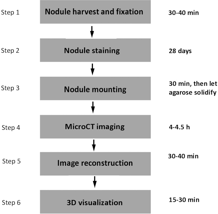
Figure 1: Protocol workflow. Overview of the workflow for using microCT to image legume root nodules and the timing required for each step. Please click here to view a larger version of this figure.
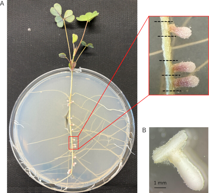
Figure 2: M. sativa root nodules for this protocol. (A) M. sativa plant 28 days after being inoculated with S. meliloti bacteria (28 dpi). Black dotted lines represent the suggested cut lines for excising the pictured nodules. Two nodules were excised per plant for three plants, and four samples were scanned. (B) M. sativa 28 dpi nodule after 4 weeks of PTA staining. Please click here to view a larger version of this figure.
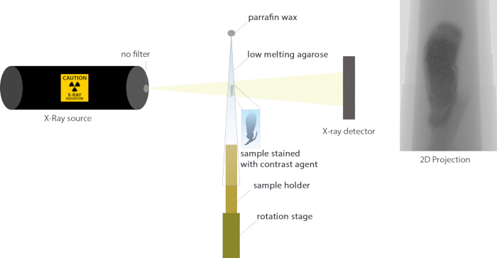
Figure 3: Overview of microCT sample set-up. The root nodule stained with a contrast agent is stabilized in low-melting-point agarose within a micropipette tip. The micropipette tip is sealed on one end with paraffin wax and secured on the rotation stage within the microCT machine. The X-ray source (no filter) is on one side of the machine, and the rays pass through the sample to reach the X-ray detector on the other side. The scan results in a 2D projection based on tissue density. Please click here to view a larger version of this figure.
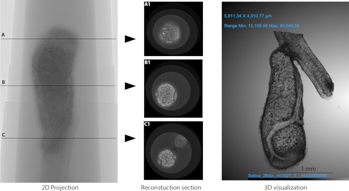
Figure 4: Example image reconstruction and 3D visualization. (Left) 2D projection. (Middle) Reconstruction section. A1, B1, and C1 show reconstructed transverse sections at locations A, B, and C from the microCT 2D projection. (Right) A 3D visualization of the root nodule produced from reconstructed images. Please click here to view a larger version of this figure.
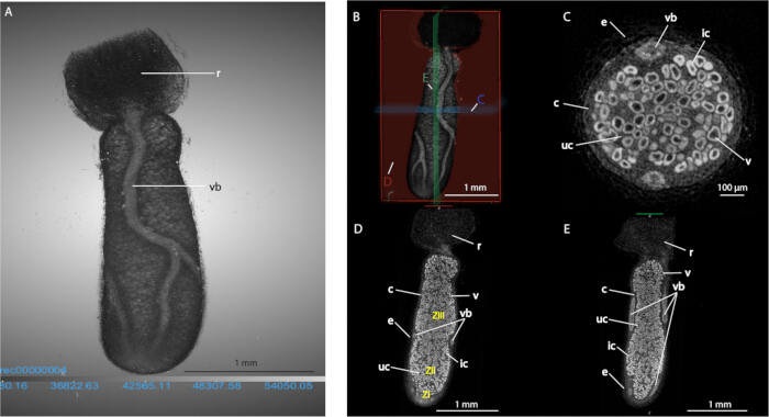
Figure 5: Annotated representative images. (A) Annotated 3D visualization of M. sativa root nodule. (B) Red, blue, and green outlines on a 3D image showing the transverse (C), coronal (D), and sagittal (E) planes, respectively. Annotated transverse (C), coronal (D), and sagittal (E) sections of M. sativa root nodule. Abbreviations: c – cortex; e – epidermis; ic – infected cell; r – root; uc – uninfected cell; v – vacuole; vb – vascular bundle; ZI – Zone I (meristematic); ZII – Zone II (infection); ZIII – Zone III (differentiation). Please click here to view a larger version of this figure.
Supplementary Figure 1. Software screenshots for microCT imaging. (A1) Open and close stage door. (A2) Turn on the camera view. (A3) Turn on X-ray source. (A4) Turn on continuous X-ray view. (A5) Adjust sample height. (A6) Adjust pixel size. (A7) Rotate sample. (A8) Change binning. (A9) Change the filter. (A10) Options to access Scanning Modes. (A11) Set the X-ray source voltage and current. (A12) Double click to turn flat-field correction off. (A13) Scanning options. (B1) Flat-field correction off. (B2) Options to access Scanning Modes. (B3) Average X-ray transmission. (B4) Adjust exposure time. (B5) Update flat-fields. (C1) Name the file and choose where to save the data. (C2) Set rotation step, frame averaging, random movement, and 360 deg scanning. (C3) Adjust partial width. (C4) Start scan.Please click here to download this file.
Supplementary Figure 2. Software screenshots for image reconstruction. (A1) Choose where to preview the sample. (A2) Preview sample. (A3) Parameter fine-tuning. (A4) Set number of trials and parameter step for post-alignment. (A5-6) Top and bottom of reconstruction area. (A7) Start reconstruction. (B1) Adjust contrast. (B2) View and click-through post-alignment results. (B3) Create circle ROI. (B4) Choose the file format and where to save the data.Please click here to download this file.
Supplementary Figure 3. Software screenshots for 3D visualization. (A) Image spacing information. (B) Selection, rotation, and zoom tools (top). Window leveling for contrast (bottom). (C) Display scale bar (top). Change background color (bottom). Please click here to download this file.
Supplementary Figure 4. MicroCT reconstruction after PTA staining for 14, 17, and 28 days. (A) Reconstructed M. sativa section after 14 d PTA staining shows noise in the outer layer (n = 1). (B) Reconstructed M. sativa section after 17 d PTA staining shows higher contrast in the outer layer but less clarity in the interior compared to (A) (n = 1). (C) Reconstructed M. sativa section after 28 d PTA staining shows higher contrast in both the outer and inner layers compared to (A) and (B) (n = 4).Please click here to download this file.
Supplementary Table 1: Parameters for microCT imaging.Please click here to download this file.
Supplementary Video 1: 3D nodule video.Please click here to download this file.
Discussion
The following are some recommendations on sample preparation and staining. During sample preparation for microCT imaging, careful excision of nodules is essential to preserve structural integrity. We recommend retaining a small segment of the root on either side of the nodule attachment point to maintain spatial context and minimize tissue damage. The use of a contrast agent is critical to enhance X-ray attenuation and visualize internal anatomical features14. A previous study using PTA staining has shown that a minimum staining period of 14 days is required to achieve sufficient contrast across different plant species and tissue types, with no evidence of overstaining14. In that study, Bradyrhizobium-induced soybean root nodules (fixed at 14 dpi) were stained for 35 days14. Using this range (14–35 days) as a reference, we performed preliminary staining trials on our own nodule samples at several timepoints (14, 17, and 28 days) and compared the resulting image contrast. A 28-day staining period was selected for this protocol, as it provided better contrast, clearer cell boundaries, and more uniform staining compared to shorter timepoints (Supplementary Figure 4). We note that the 14- and 17-day reconstructions come from a single nodule rather than a systematic replicate study, while the 28-day condition includes all four scanned nodules, and the staining duration should be adjusted based on the resolution needed for the study. A 28-day staining period is also not a short time frame. As suggested in previous studies, microwave-assisted staining may help accelerate PTA penetration and thereby shorten the required staining duration14. Iodine-based agents, such as Lugol’s solution, are also used to enhance contrast in plant tissue23,24. We selected PTA on the basis of its demonstrated performance in nodule tissue and did not compare staining agents, as the main aim of this study was to establish a single reproducible protocol14. Future studies should test other stains across different plant species and tissue types.
Proper embedding is equally important. The sample should remain completely covered with low-melting-point agarose to prevent dehydration and maintain its natural morphology. Following embedding, samples should be stored overnight at 4 °C to ensure the solidification of the agarose to maintain stability during scanning. The mounted sample must be securely fastened to the scanning stage to prevent drift or vibration artifacts during data acquisition.
MicroCT allows non-destructive, three-dimensional visualization of whole nodule tissue at a resolution coarser than both light and electron microscopy. Both XRM and synchrotron-based X-ray CT generally provide higher quality and resolution images than conventional microCT. Synchrotron-based X-ray CT can also allow fresh, unstained samples to be scanned directly, as high photon flux and beam coherence permit rapid acquisition and sufficient contrast without contrast-enhancing agents6. Direct comparison with Duncan et al. (2022)14 and Nakhforoosh et al. (2024)6 is limited by differences in study design: species (soybean vs Medicago sativa), nodule type (determinate vs indeterminate), and imaging modality (XRM and synchrotron-based X-ray CT vs conventional microCT). Nevertheless, the nominal pixel size of our nodule reconstructions is approximately 1.75 µm, finer than the nodule scan in Duncan et al. (2022)14 (2.2 µm, Figure 4A), yet their reconstructions still show greater clarity than ours. This likely reflects that effective resolution depends on more than nominal pixel size; the optical magnification of the XRM's objective lenses, detector sensitivity, source stability, camera quality, and reconstruction methods all contribute. While large, low-density features such as vacuoles are readily distinguishable, as shown here, occupancy of individual cells by bacteroids and smaller or less dense organelles is not, and dynamic biological processes cannot be captured in real time. PTA and iodine-based contrast agents are non-specific and cannot report molecular identity. Subcellular questions will still require fluorescence or electron microscopy. These imaging approaches are complementary, with microCT well-suited to whole-organ morphology and 3D tissue architecture, providing context for light and electron microscopy, which address finer structural and molecular detail.
We have successfully replicated this workflow with nodules at similar time points and developmental stages from M. sativa inoculated with other S. meliloti strains, and M. truncatula and Trigonella foenum-graecum inoculated with several different S. meliloti strains (unpublished data). We did not test nodules of different developmental stages, as our aim was to characterize and provide a reproducible protocol for mature, nitrogen-fixing nodules. Even so, the workflow should be applicable to nodules of varying developmental stages, as the more relevant limitation is nodule size. The nodules we scanned were approximately 2.5 mm in length (Supplementary Table 1). On the microCT used in this study, the smallest we recommend is 1 mm in length. The size that can be imaged will be affected by the machine used, as magnifications may vary.
Recent evidence suggests that occupancy within the nodule is an important parameter that directly correlates with nitrogen fixation efficiency. Nodules with a greater proportion of infected cells have been shown to fix nitrogen better than the ones in which fewer cells are occupied by bacteria25. Additionally, nodule health depends on the extent of vasculature, and disrupted or limited vasculature implies defective nodules and reduced plant health26. Given the potential to visualize occupancy and vascular architecture, microCT fills an important gap in the field of nitrogen fixation. This workflow makes non-destructive visualization of the interior and exterior structures of root nodules routinely accessible, and those structures are direct determinants of the fixation efficiency that drives symbiotic nitrogen supply to crops.
Disclosures
The authors have nothing to disclose.
Acknowledgements
We would like to thank Stephanie Sage for her help with plant preparation. Xia Zhao helped with sample embedding. We are grateful to Madi Mitchell for the initial project discussion. We would like to thank Tom Kleist and Kexi Yi for their data interpretation advice. We also thank Keith Duncan (Donald Danforth Plant Science Center) for his protocol advice. This project is funded by the Stowers Institute for Medical Research.
Materials
| Name | Company | Catalog Number | Comments |
|---|---|---|---|
| 20 mL Glass vial | Sigma-Aldrich | Z190527 | Used to hold nodules for fixation and staining. |
| 200 µL Pipette tips | Fisherbrand | 02-717-144 | Used to hold nodules for imaging. |
| 35 mm Microwell dish | Fisher Scientific | 507532924 | Used to wash nodules after staining. |
| Dragonfly Software | Comet Technologies Canada Inc. | V2022.2 | Used to visualize and manipulate 2D reconstructions in a 3D view. |
| Ethanol | Decon Labs | V1001 | Used to fix and wash nodules. |
| Fine forceps | Dumont | AA-Inox-E | Used to adjust nodules in the pipette tip. |
| Gel load tip | Corning (Costar) | 4853 | Used to manipulate the nodule within the agarose inside the pipette tip. |
| Hot plate | Mirak | SP72725 | Used to melt paraffin and dissolve lowMelt agarose. |
| LowMelt agarose | GeneMate | 490001-602 | Used for root nodule embedding to maintain orientation and moisture. |
| MicroCT | Bruker | Bruker SkyScan 1272 | Used for scanning the nodule. |
| NRecon Software | Bruker | V2.2.0.6 | Used for the reconstruction of 2D projections. |
| Orbital shaker | VWR | 77591-858 | Used for shaking the root nodule to accelerate the staining penetration. |
| Paraffin | McCormick Scientific | 39503002 | Used to seal narrow end of pipette tip. |
| Parafilm | Alkali Scientific | PM996 | Used to seal pipette tips to prevent sample from drying out. |
| Phosphotungstic acid | Electron Microscopy Science (EMS) | 19500 | Used for nodule staining. |
| Sample holder - L 3.4 cm D 0.63 mm | Bruker | Set from Bruker with machine | Used to hold pipette tip and sample during imaging. |
| Scalpel | Fisher Scientific | S07890 | Used to harvest root nodules. |
| Skyscan software | Bruker | v1.5.1.0 | Used for manipulating the MicroCT. |
| Water bath | Boekel Grant | 640013001 | Used to keep agarose liquid while embedding nodules. |
References
- Oldroyd GED, Murray JD, Poole PS, Downie JA. The rules of engagement in the legume-rhizobial symbiosis. Annu Rev Genet. 2011;45:119-44.
- Gibson KE, Kobayashi H, Walker GC. Molecular determinants of a symbiotic chronic infection. Annu Rev Genet. 2008;42:413-41.
- Porter SS, et al. Host-imposed control mechanisms in legume-rhizobia symbiosis. Nat Microbiol. 2024;9:1929-39.
- Guerra-García FJ, Sankari S. NCR peptides in plant-bacterial symbiosis: applications and importance. Trends Microbiol. 2025;33(2):147-50.
- Rae AE, Rolland V, White RG, Mathesius U. New methods for confocal imaging of infection threads in crop and model legumes. Plant Methods. 2021;17:24.
- Nakhforoosh A, et al. Visualization and quantitative evaluation of functional structures of soybean root nodules via synchrotron X-ray imaging. Plant Phenomics. 2024;6.
- Nierenberger M, Rémond Y, Ahzi S, Choquet P. Assessing the three-dimensional collagen network in soft tissues using contrast agents and high resolution micro-CT: Application to porcine iliac veins. C R Biol. 2015;338(7):425-33.
- Livingston D, Tuong T, Nogueira M, Sinclair T. Three-dimensional reconstruction of soybean nodules provides an update on vascular structure. Am J Bot. 2019;106(3):507-13.
- Warner CA, et al. An optical clearing technique for plant tissues, allowing deep imaging and compatible with fluorescence microscopy. Plant Physiol. 2014;166(4):1684-7.
- Indore NS, Karunakaran C, Jayas DS. Synchrotron tomography applications in agriculture and food sciences research: a review. Plant Methods. 2022;18:101.
- Novák K. Determination of symbiotic nodule occupancy in the model Vicia tetrasperma using a fluorescence scanner. Ann Bot. 2011;107(4):709-15.
- Martin L, et al. Cancer cachexia in the age of obesity: Skeletal muscle depletion is a powerful prognostic factor, independent of body mass index. J Clin Oncol. 2013;31(12):1539-47.
- Liguori C, et al. Emerging clinical applications of computed tomography. Med Devices (Auckl). 2015;8:265-78.
- Duncan KE, et al. X-ray microscopy enables multiscale high-resolution 3D imaging of plant cells, tissues, and organs. Plant Physiol. 2022;188(2):831-45.
- Wang J, et al. A deep learning-based micro-CT image analysis pipeline for nondestructive quantification of the maize kernel internal structure. Plant Phenomics. 2025;7(1).
- Brackin R, Atkinson BS, Sturrock CJ, Rasmussen A. Roots-eye view: Using microdialysis and microCT to non-destructively map root nutrient depletion and accumulation zones. Plant Cell Environ. 2017;40(12):3135-42.
- Brodersen CR, Roddy AB. New frontiers in the three-dimensional visualization of plant structure and function. Am J Bot. 2016;103(2):184-8.
- Schoborg TA, et al. Micro-computed tomography as a platform for exploring Drosophila development. Development. 2019;146(23).
- Wang M, et al. Nanoplastics causes extensive congenital malformations during embryonic development by passively targeting neural crest cells. Environ Int. 2023;173.
- Brodersen CR, et al. The dynamics of embolism repair in xylem: In vivo visualizations using high-resolution computed tomography. Plant Physiol. 2010;154(3):1088-95.
- Brodersen CR, et al. In vivo visualizations of drought-induced embolism spread in Vitis vinifera. Plant Physiol. 2013;161(4):1820-9.
- Nolf M, et al. Visualization of xylem embolism by X-ray microtomography: a direct test against hydraulic measurements. New Phytol. 2017;214(2):890-8.
- Karahara I, Yamauchi D, Uesugi K, Mineyuki Y. Three-dimensional visualization of plant tissues and organs by X-ray micro-computed tomography. Microscopy (Oxf). 2023;72(4):310-25.
- Staedler YM, Masson D, Schönenberger J. Plant tissues in 3D via X-ray tomography: simple contrasting methods allow high resolution imaging. PLoS One. 2013;8(9).
- Sánchez-Cañizares C, et al. Developmental fates and N2-fixing efficiency of terminally-differentiated versus undifferentiated bacteroids from legume nodules. Plant Physiol. 2026;200(3).
- Pepper AN, Morse AP, Guinel FC. Abnormal root and nodule vasculature in R50 (sym16), a pea nodulation mutant which accumulates cytokinins. Ann Bot. 2007;99(4):765-76.
Reprints and Permissions
This article has been published
Video Coming Soon