Extracellular Electrophysiological Recording of Visually Evoked Swim Pacemaker Signals from the Isolated Rhopalium of Tripedalia cystophora

Summary

This protocol describes extracellular electrophysiological recording of visually evoked swim pacemaker signals from the isolated rhopalium of the box jellyfish Tripedalia cystophora, providing a quantitative readout of obstacle avoidance behavior for precise investigation of visual information processing and sensorimotor integration.

Abstract

The box jellyfish Tripedalia cystophora combines image-forming lens eyes and well-characterized visually guided behaviors with a tractable rhopalial nervous system of approximately 1000 neurons, making it an emerging model for systems-level investigation of visual information processing and sensorimotor integration. Swim pacemaker neurons generate motor commands directly controlling bell contractions, and these signals can be recorded extracellularly from the epidermal stalk nerve of an isolated rhopalium, providing a quantitative proxy for visually driven motor output. The strength of the pacemaker response, quantified as standardized neural activity derived from pacemaker signal count and instantaneous frequency, scales with stimulus contrast above the decision transition threshold (DTT), enabling graded evaluation of visually driven sensorimotor integration. In this protocol, we cover the fabrication of extracellular suction electrodes, rhopalial isolation, recording chamber configuration, visual stimulus delivery to the lower lens eye, hardware-level stimulus timing verification, electrode placement on the epidermal stalk nerve, and synchronized electrophysiological and stimulus data acquisition using standard laboratory hardware.

Introduction

Understanding how nervous systems process sensory information and translate it into adaptive behavior is a central challenge in neuroscience. Progress has been substantial in large, complex model organisms, such as Drosophila melanogaster, whose brain of approximately 200,000 neurons has enabled detailed dissection of neural circuit organization¹, among other genetically tractable models with sophisticated imaging and circuit-mapping tools. However, the very complexity of these systems makes it difficult to achieve a complete, systems-level understanding of the relationship between sensory input, neural computation, and behavioral output. At the other end of the complexity spectrum, small fully mapped systems, such as that of Caenorhabditis elegans, comprising 302 neurons², among other minimal-neuron-count models, offer tractable size but lack image-forming eyes and the visually guided behaviors that depend on them.

Tripedalia cystophora, the Caribbean box jellyfish (Figure 1A), is emerging as a model system for systems-level visual information processing and sensorimotor integration, occupying a distinctive position between these extremes³. The protocol described here (Figure 1) is designed to make the full experimental potential of this animal accessible to the wider neuroscience community.

T. cystophora possesses a visual system of remarkable sophistication for an animal of its neural complexity. Each of the four sensory structures called rhopalia carries six eyes, including two image-forming lens eyes: the upper lens eye (ULE) and the lower lens eye (LLE)⁴ (Figure 1B). These are not simple photoreceptive organs — they are equipped with a graded refractive index lens of the Matthiessen type, a lens design also found in vertebrate eyes, and an everted retina in which approximately 600 photoreceptors in the LLE and 400 in the ULE articulate directly onto second-order neurons^5,6,7. The molecular composition of the photoreceptive machinery, including cnidops opsins homologous to vertebrate c-opsins and associated phototransduction components^8,9,10, strongly suggests that these are hyperpolarising photoreceptors, placing the T. cystophora visual system in the same broad functional category as the vertebrate eye despite its independent evolutionary origin.

Critically, these optical investments are matched by elaborate, experimentally characterizable, visually guided behaviors. T. cystophora navigates the optically complex mangrove habitat using long-distance navigation and light shaft detection mediated to maintain position within the habitat^11,12, and obstacle avoidance behavior to navigate around submerged prop roots^12,13,14. The neuroethological framework underlying this work holds that behavior is the only valid readout of sensory processing in non-linguistic animals. Since we cannot ask animals what they perceive, the experimental design must be adapted to stimuli the animal can detect and understand, and to behaviors the animal is capable of performing. This implies that experimental questions must be formulated on the animal's terms, not the investigator's. The obstacle avoidance behavior of T. cystophora exemplifies this principle. The box jellyfish epidermis is only a single cell layer thick, making collision with a submerged prop root potentially fatal due to damage to its fragile body. Since inter-rhopalial integration occurs only downstream via the ring nerve¹⁵, no single rhopalial nervous system (RNS) receives the overlapping binocular input required to compute depth from stereoscopic disparity. Instead, the animal exploits a fundamental property of underwater optics: contrast between an object and the surrounding water dissipates rapidly with increasing distance. A high-contrast obstacle is therefore a close obstacle, one that poses an immediate threat, while a low-contrast obstacle is distant and not yet threatening. The animal uses contrast as a proxy for distance¹⁶. In freely behaving animals, obstacle avoidance behavior (OAB) is based on a go/no go decision; an event is triggered when the animal detects an underwater obstacle whose contrast exceeds the decision transition threshold (DTT), the threshold above which the obstacle is sufficiently close to constitute a threat, and initiates the go response: 3–5 rapid bell contractions, a 120–180° turn, and rapid swimming away from the obstacle¹⁴ (Figure 1C). The graded pacemaker response above the DTT reflects the graded urgency of the threat¹⁶. The OAB thus provides a highly tractable behavioral assay for sensorimotor integration: a single, well-defined visual parameter (contrast) controls a stereotyped, quantifiable motor output, making it an ideal system for investigating the neural basis of visually driven decision-making.

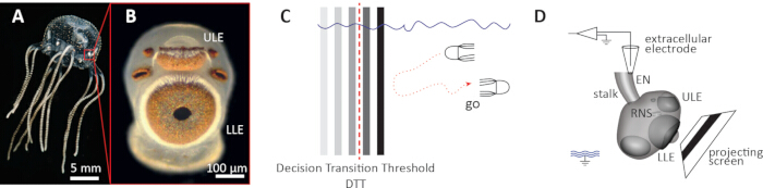
Figure 1: Overview of the Tripedalia cystophora isolated rhopalium preparation for extracellular electrophysiological recording. (A) Adult T. cystophora medusa. Scale bar: 5 mm. The red box indicates the position of one rhopalium on the bell margin. (B) Close-up of an isolated rhopalium. The upper lens eye (ULE) and lower lens eye (LLE) are image-forming eyes. Scale bar: 100 µm. Image by Dan-Eric Nilsson, reproduced with permission. (C) Schematic illustration of the obstacle avoidance behavior (OAB). Below the decision transition threshold (DTT, red dashed line), the animal continues swimming toward the obstacle (no go). Above the DTT, obstacle avoidance behavior is initiated (go). (D) Schematic of the isolated rhopalium electrophysiology preparation. The rhopalium is positioned facing the inclined projecting screen. The extracellular electrode records swim pacemaker signals from the epidermal stalk nerve (EN). RNS: rhopalial nervous system; ULE: upper lens eye; LLE: lower lens eye; EN: epidermal stalk nerve. The ground symbol indicates the bath reference electrode. Please click here to view a larger version of this figure.

The neural substrate mediating this visual processing is the RNS, comprising approximately 1000 neurons per rhopalium¹⁷. Despite this limited neuron number, the RNS is architecturally sophisticated. Immunohistochemical evidence suggests that it is organized into discrete clusters of neurons expressing distinct neuropeptide profiles¹⁸, consistent with a compartmentalized processing architecture. It is suggested that visual information is processed through subordinate oscillatory clusters (subOCs), each associated with a specific eye on the rhopalium, which converge onto a terminal oscillatory cluster (trmOC) — proposed to correspond to the pacemaker cell population that generates the motor output signal controlling bell contractions³. We propose that the trmOC integrates processed sensory information from the subOCs and generates the swim pacemaker signal that drives behavioral motor output, and that synchronization between subOCs and the trmOC underlies the transformation of visual input into behavioral control output³ (Figure 2).

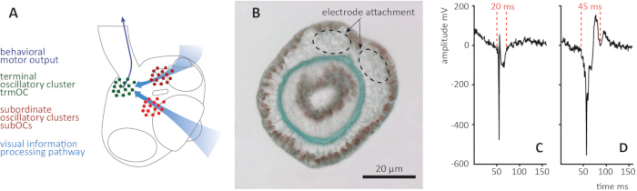
Figure 2: Neural circuit origin and electrophysiological identification of the swim pacemaker signal in Tripedalia cystophora. (A) Schematic of the rhopalial nervous system. Visual information is processed through subordinate oscillatory clusters (subOCs, red) associated with the individual eyes, and converges onto the terminal oscillatory cluster (trmOC, green). It is proposed that the trmOC integrates processed sensory information from the subOCs and generates the swim pacemaker signal that drives behavioral motor output. Light blue arrows indicate the visual information processing pathway; the dark blue arrow indicates behavioral motor output. (B) TEM micrograph of the transected epidermal stalk surface. Dashed circles indicate the two attachment points of the bifurcated epidermal stalk nerve on the adoral surface of the stalk, corresponding to the sites of recording electrode placement. (C) Action potential-like signal. The waveform is characterized by a sharp, narrow deflection with a duration of approximately 20 ms (indicated by red dashed lines). (D) Swim pacemaker signal originating from the trmOC. The waveform is broader, with a characteristic duration of approximately 45 ms (indicated by red dashed lines), and displays a compound morphology reflecting the summed activity of multiple trmOC neurons. Although signal amplitudes are comparable between the two signal types, waveform duration and morphology are the reliable discriminating criteria for downstream analysis. All electrophysiological values are post-amplification (×1000). Modified with permission from Bielecki et al.²⁴. Please click here to view a larger version of this figure.

This architecture creates an exceptional experimental opportunity. The swim pacemaker signal generated by the trmOC drives bell contractions in a strict one-to-one manner¹⁹ and can be recorded extracellularly from the epidermal stalk nerve of an isolated rhopalium^13,20. This means that visually evoked motor commands, and by extension, visually guided behavioral responses, can be monitored using electrophysiological methods in a preparation from which the motor effectors themselves have been entirely removed¹⁴. The isolated rhopalium thus occupies a methodological middle ground that is difficult to achieve in other systems: it offers the experimental control of a reduced preparation, including precise specification of spatio-temporal visual stimuli, while retaining a direct, quantitative readout of behavior-relevant neural output. During undisturbed conditions, pacemaker signals occur at 0.5–1 Hz; visually evoked obstacle avoidance responses are characterized by increases to 2–3 Hz, providing a clear signal window for analysis¹⁴ (Figure 1D).

This combination of properties makes the T. cystophora isolated rhopalium preparation well-suited for systems-level investigation of visual processing and sensorimotor integration. This preparation is appropriate for researchers seeking to investigate visual processing, sensorimotor integration, or oscillatory network dynamics in a tractable nervous system with image-forming eyes and well-characterized visually guided behaviors⁴. It requires standard electrophysiology equipment, a modified commercial projector, and a dissection microscope, and can be established in a laboratory without specialist infrastructure. The associative mechano-visual learning paradigm — the associative pairing of concurrent visual and mechanosensory stimulation — previously described for this preparation¹⁴ can be implemented as an extension of the basic recording protocol described here.

Protocol

No animal ethics approval was required for this study. Cnidarians, including Tripedalia cystophora, fall outside the scope of Directive 2010/63/EU on the protection of animals used for scientific purposes, which applies to cephalopods and vertebrates only. Animals used in this study were collected from mangrove creeks off La Parguera, Puerto Rico, USA, which is not a Party to the Nagoya Protocol on Access to Genetic Resources and Benefit-Sharing; no prior informed consent or access and benefit-sharing agreement was therefore required. Tripedalia cystophora is not listed as endangered or protected under CITES or any applicable national conservation legislation.

1. Stage and signal chain setup

NOTE: All hardware components and their connections are illustrated in Figure 3. Refer to Figure 3 throughout this section. All steps in this section must be completed before the animal is handled. The recording chamber is not filled with seawater at this stage.

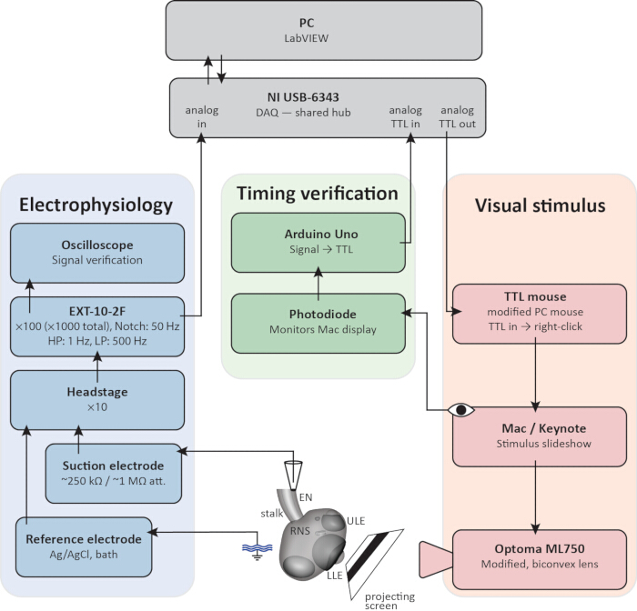
Figure 3: Connection diagram for the isolated rhopalium extracellular electrophysiology preparation. The PC running VI and the DAQ (top, gray) serve as the shared integration hub for all three signal chains. Electrophysiology chain (blue): Swim pacemaker signals are recorded from the epidermal stalk nerve (EN) via a suction electrode (~250 kΩ free tip, ~1 MΩ attached) and bath-applied Ag/AgCl reference pellet electrode, amplified by the EXT-10-2F headstage (×10) and main amplifier (×100, total ×1000) with bandpass (HP: 1 Hz, LP: 500 Hz) and 50/60 Hz notch filtering, monitored on the oscilloscope, and acquired by the DAQ. Visual stimulus chain (red): A DAQ TTL pulse advances the stimulus slideshow via a modified PC mouse (TTL mouse), driving the DLP projector (modified, biconvex lens) to project the stimulus onto the inclined screen wall of the recording chamber in front of the lower lens eye (LLE). Timing verification chain (green): A photodiode monitors the black and white indicator square on the computer display that switches from white to black at stimulus onset and returns to white at offset; an Arduino Uno converts this signal to a TTL pulse recorded by the DAQ as the verified stimulus window. RNS: rhopalial nervous system; ULE: upper lens eye; LLE: lower lens eye; EN: epidermal stalk nerve. All amplitude values are post-amplification (×1000). Please click here to view a larger version of this figure.

1. Recording chamber construction
   1. Design or 3D print a recording chamber of sufficient internal dimensions to accommodate the preparation, the holding micropipette tip, and the recording electrode tip.
      NOTE: The functionally critical design features are the coverslip ledge, which positions the rhopalium at the coverslip edge 2 mm from the projection screen, and the screen dimensions (16 mm × 12 mm, inclined at 60°), which together determine the angular subtense of the visual stimulus at the lower lens eye. The chamber described here has a base footprint of 30 mm ×3 0 mm and a wall thickness of approximately 5 mm. Technical drawings are provided in Figure 4.
   2. Place the Roth 20 mm × 26 mm hemacytometer coverslip on the coverslip ledges of the recording chamber. The coverslip rests in place by negative buoyancy and requires no adhesive fixation.
   3. Mount the recording chamber on the microscope stage using the M6 through-holes. An x-y-z translational stage is recommended, as it facilitates fine alignment of the projected image onto the projection screen wall of the recording chamber.
   4. Connect the inlet and outlet ports of the recording chamber flow-through channels (Figure 4A) to a temperature-controlled water bath circulating water at 28 °C.
      NOTE: The recording chamber temperature should be maintained within 28–30 °C throughout the experiment.
2. Optical configuration (Figure 3, visual stimulus chain)
   CAUTION: Do not view the projector output directly, particularly before neutral density filters are installed (Section 4). Removal of the manufacturer's lens system removes built-in light attenuation and may cause eye injury.
   1. Remove the manufacturer's lens system from the projector.
   2. Mount a single biconvex lens (f = 30 mm) in front of the projector output aperture to focus the projected image onto the projection screen wall of the recording chamber.
   3. Align the projector such that the projected image is in focus on the projection screen wall of the recording chamber and fills the screen dimensions (16 mm × 12 mm).
      NOTE: Neutral density filters are not inserted at this stage. The appropriate filter strength is determined empirically during the biological calibration in Section 4.
3. Signal chain assembly (Figure 3, electrophysiology and timing verification chains)
   1. Connect the electrode holder to the headstage arm supplied with the EXT-10-2F amplifier and secure the headstage arm in one MM33 micromanipulator.
   2. Connect the headstage to the main amplifier. The headstage gain is ×10. Set the main amplifier gain to ×100, yielding a total amplification of ×1000.
   3. Connect the amplifier output to an analog input channel of an analog-digital converter (DAQ).
   4. Connect the DAQ to the PC running LabVIEW (version 2018 or similar) via USB.
   5. Connect the Arduino Uno TTL output to a dedicated analog input channel of the DAQ.
   6. Position the photodiode over the black and white indicator square on the computer display (step1.4.2). Connect the photodiode's positive terminal to Arduino Uno analog input pin A0 and the negative terminal to ground. The Arduino sketch implementing the photodiode monitoring and TTL output threshold logic is provided as supplementary material (Supplementary File 1).
4. Stimulus geometry design (Figure 3, visual stimulus chain)
   1. Design the visual stimulus in the presentation software as a moving vertical gray bar on a white background, mimicking a mangrove prop root obstacle. Set the background to maximum white.
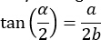
      NOTE: The gray level of the bar relative to the white background determines the contrast of the stimulus and is established during irradiance characterization in Section 4. The bar should subtend 30° of visual angle of the lower lens eye (measured at the center of the visual field) and move at 10° s^-1 across the full width of the visual field, remaining within the visual field at all times. The visual angle of a projected obstacle can be determined by:
      
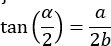
      where α is the visual angle, a is the width of the image feature, and b is the distance from the lower lens eye to the screen. The bar's motion is implemented as a single continuous object animation (e.g., Keynote's "Move" build) applied to the bar object within one slide, rather than as a sequence of discrete slides. A representative stimulus file implementing this animation is provided as supplementary material (Supplementary File 2). Because bar width and speed are specified in visual angle rather than physical units, both must be converted to millimeters and mm/s using the equation above, based on the specific working distance and screen dimensions of the recording chamber, before being entered as the animation's object size and duration in the presentation software.
   2. Include a small black and white indicator square in a corner of the slide that switches from white to black coinciding with the onset of bar movement and returns to white at stimulus offset. Monitor this square on the computer display using the photodiode for stimulus timing verification in step 3.3.
      NOTE: The black and white indicator square necessarily appears within the projected image on the recording chamber screen, as it must be part of the slide to appear on the computer display during presentation. However, the square is sized to fill only the photodiode receptive area on the computer display. When projected onto the chamber screen, it is sufficiently small that it is not resolvable as a distinct visual feature by the lower lens eye, and its contribution to overall screen luminance is negligible and does not initiate light ON/OFF responses^4,13,20.
   3. Advance the presentation software slides using either an automated or manual trigger.
      1. Option A (automated): Construct a transistor-transistor-logic (TTL) mouse by modifying a standard PC mouse such that a brief 5 V TTL pulse received from the DAQ output replaces a right-click signal. Connect the TTL mouse to the presentation computer via USB. Configure the presentation software to advance slides on a right-click input.
      2. Option B (manual): Manually trigger slide advancement at the intended stimulus onset. Because the Arduino-verified stimulus window (Channel 3), rather than the triggering signal itself, is used as the definitive timing record for analysis (step 6.2.1), manual triggering does not compromise timing accuracy, though it requires precise operator timing during acquisition and is less convenient than the automated option.

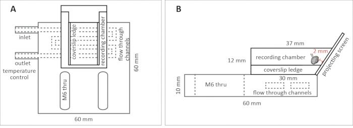
Figure 4: Recording chamber for the isolated rhopalium preparation. (A) Top view schematic. The recording chamber is flanked by flow-through channels for water-jacket temperature control, with inlet and outlet ports (OD 4.2 mm, ID 2.5 mm) indicated. The coverslip ledges run longitudinally along both internal walls of the chamber, supporting the hemacytometer coverslip at mid-chamber height. M6 through-holes provide mounting points for securing the chamber to the microscope stage. Overall dimensions: 60 mm × 60 mm. (B) Side view schematic with dimensions. The recording chamber has an internal height of 12 mm and a top width of 37 mm. One wall of the chamber forms the projection screen, inclined at 60° relative to vertical to align with the optical axis of the lower lens eye. The coverslip ledge positions the rhopalium at the coverslip edge facing the projection screen. The 2 mm working distance shown reflects the specific chamber, screen, and projector configuration described in this protocol; readers adapting this design to different hardware should recalculate an appropriate working distance for their own setup using the equation in step 1.4.1. Flow-through channels for temperature control run within the recording chamber base and do not contact the preparation. Please click here to view a larger version of this figure.

2. Electrode fabrication

NOTE: Extracellular suction electrodes consist of glass capillary tubes with tapered tips pulled to create an opening suitable for suction adhesion and recording of electrical potentials. The glass capillary serves as electrical insulation, ensuring that only potentials at the tip are recorded. A silver wire inserted into the capillary connects to the amplifier. This configuration achieves multi-unit recordings, capturing electrical potentials from groups of pacemaker cells at the electrode tip measured against a bath-applied reference electrode. Electrodes should be fabricated on the day of use, prior to the recording session. Stored electrodes are prone to tip occlusion, which prevents seawater from being drawn into the capillary and renders the electrode non-functional. Pulled glass capillaries have sharp, fragile tips. Handle with care during fabrication to avoid puncture injury, and dispose of broken, rejected, or used capillaries in a designated sharps container.

1. Pulling the glass capillary tube
   1. Load a borosilicate glass capillary tube (1.16 mm ID × 2.00 mm OD × 80 mm L) into the micropipette puller.
   2. Execute the following pulling program: Line 1 (×1): heat 535, pull 0, velocity 12, time 200, pressure 600, ramp 540. Lines 2–4 (×3): heat 532, pull 0, velocity 12, time 100.
      NOTE: These parameters are specific to the instrument, glass, and filament used and may require adjustment on a different unit or after filament wear; treat them as a starting point rather than a fixed specification.
   3. Remove the pulled electrode carefully and store it tip-up to prevent mechanical damage.
2. Polishing the electrode tip
   1. Polish the tip to create a smooth, vacuum-seal surface perpendicular to the capillary axis. Refer to the two options provided below; Option A (microforge) is recommended.
   2. Option A: Polishing with a microforge (recommended)
      1. Mount the pulled electrode in a microforge.
      2. Under 600× magnification (40× objective, 15× ocular), position the tip near the heating filament.
      3. Heat and polish the tip until the opening measures approximately 250 kΩ resistance (corresponding to ~1 MΩ when in contact with tissue). At 600× magnification, this corresponds to approximately three increments on the eyepiece reticle scale.
         NOTE: To measure electrode resistance, connect a multimeter between the BNC core (connected to the electrode's silver wire) and the bath reference (Ag/AgCl pellet) electrode, once the electrode has been filled with seawater. Electrical resistance measurement is not required for standard visually evoked recordings, where signal quality is the primary criterion for electrode adequacy (step 6.1.5); it becomes necessary when this preparation is used for the associative learning paradigm requiring calculated current delivery, which is outside the scope of this protocol¹⁴.
      4. Allow the electrode to cool completely before removing it from the microforge.
   3. Option B: Manual polishing without a microforge
      CAUTION: This step uses an open flame (ethanol burner). Keep flammable materials clear of the flame and follow standard laboratory open-flame precautions.
      1. Briefly hold the pulled capillary tip in the flame of an ethanol burner until the glass melts and seals the tip as a fine droplet.
      2. Allow the sealed tip to cool completely.
      3. Place a drop of deionized water on a sheet of fine sandpaper (1200 grit) and hold the capillary perpendicular to the paper surface.
      4. Sand the tip using small circular motions, alternating between clockwise and counterclockwise directions.
      5. Continue sanding carefully until a small amount of glass debris-laden water is drawn into the tip by capillary action.
      6. Attach a rubber tube to the opposite end of the capillary and connect it to a syringe.
      7. Apply gentle suction to draw deionized water through the tip, flushing out glass debris.
      8. If debris does not clear, sand gently for a brief additional period and repeat the flushing step.
         NOTE: The target flow rate through the finished tip is approximately 1 cm of water column per 10 s under gently applied suction.Tip fabrication success is defined by recording outcome (low-noise, high-amplitude signal), not by tip appearance. Approximately 40%–50% of fabricated electrodes for either polishing option yield such recordings, though the limiting factor differs between them. For microforge polishing (Option A), failure most commonly traces back to uneven pore geometry arising during the pulling step (step 2.1), which subsequent heat-polishing cannot fully correct. For manual polishing (Option B), success depends primarily on operator skill; the most common failure is an oversized pore from over-sanding. A smooth, correctly sized, round pore substantially increases the probability of a high-quality recording, but does not guarantee it — the functional outcome is the only criterion that ultimately matters.
3. Assembling the electrode
   1. Insert the polished capillary tube into the electrode holder, making sure that the Ag/AgCl (silver/silver chloride) wire is extended and without kinks within the glass capillary, and mount it in the headstage arm supplied with the EXT-10-2F amplifier. Secure the headstage arm in the MM33 micromanipulator.
      NOTE: If the silver wire is not chlorided, chloride it electrochemically by immersing both the electrode's silver wire and a separate solid silver electrode in 2 M KCl solution, connected via insulated leads to a 12 V DC source. Apply the current in approximately 2-min intervals, visually inspecting the wire between rounds; the wire is sufficiently chlorided once it has visibly darkened, typically within 5 min total. Rinse thoroughly with deionized water after chloriding. An unchlorided wire can introduce a large and unstable DC offset.
      CAUTION: Electrolytic chloriding in KCl solution generates chlorine and hydrogen gas. Perform in a ventilated area. Dispose of used KCl chloriding solution in accordance with institutional hazardous waste guidelines.
   2. Fill the electrode immediately prior to recording by drawing seawater directly from the filled recording chamber into the capillary until the internal solution reaches halfway up the silver wire. See step 3.1 for the filling procedure.
      NOTE: Holding micropipettes does not require the optical or electrical specifications of recording electrodes. Electrodes rejected during fabrication (step 2.2) due to excessive tip diameter (resistance below 250 kΩ) or off-center tip geometry are suitable for this purpose and should be retained. Fabricating dedicated holding micropipettes is unnecessary.

3. System validation

This section verifies that the complete recording system — electrode, signal chain, stimulus delivery, and timing verification — is functioning correctly before the experimental preparation is introduced. The complete signal chain is illustrated in Figure 3. Verify that all connections are in place before proceeding.

1. Chamber filling and electrode preparation
   1. Fill the recording chamber with 0.20 µm filtered seawater from the culture tank. This ensures continuity in the chemical composition between the culture environment and the recording chamber, preventing exposure of the rhopalium to foreign compounds or changes in water chemistry that could affect pacemaker activity or preparation viability.
   2. Fill the recording suction electrode by drawing seawater directly from the recording chamber into the capillary until the internal solution reaches halfway up the silver wire. Fill the holding micropipette with sufficient seawater from the recording chamber to enable suction adhesion to the crystal.
   3. Place an Ag/AgCl (silver/silver chloride) sintered pellet electrode in the recording bath and connect to the reference input of the headstage.
2. Grounding and noise verification
   CAUTION: This setup operates electrical equipment in close proximity to seawater. Keep all electrical connections and equipment away from the chamber and any spills, and follow institutional electrical safety practices for wet-environment work.
   1. Ground all instruments to a single common earth point (star grounding configuration) to prevent ground loops.
   2. Monitor the signal on the oscilloscope. Verify that the baseline is clean and noise-free before proceeding.
      NOTE: Faraday cages are generally not used in our lab for extracellular recordings, since rigorous star grounding consistently proves more effective at eliminating electrical (50/60 Hz)noise than physical shielding.
3. Timing verification chain
   1. Run the LabVIEW virtual instrument (VI) (supplied as supplementary material, Supplementary File 3). Run the VI during system validation. This sends the TTL pulse to the TTL mouse to trigger the stimulus build, and generates a .txt output file that allows verification that all channels — electrophysiological signal, LabVIEW TTL, and Arduino TTL — are correctly acquired before the experimental preparation is introduced.
      NOTE: The delay between the LabVIEW-logged TTL command and the Arduino-verified stimulus onset varies unpredictably between recordings and is not resolved at this stage; it is instead determined and corrected for individually in each recording during analysis (step 7.2.1).
   2. Verify that the TTL pulse from the DAQ correctly triggers the stimulus build and that the visual stimulus is delivered to the projection screen as designed.
   3. Verify that the Arduino Uno detects the change in the black and white indicator square on the computer display and outputs a TTL pulse to the DAQ.
      NOTE: The Arduino Uno samples the photodiode voltage via analogRead(A0). When the sampled value falls below an empirically determined threshold (61 out of the 0–1023 analogRead range in this setup), digital output pin 5 is set to 5 V (TTL high); when the value returns above threshold, the output returns to 0 V. This threshold is setup-dependent and must be recalibrated for each screen and ambient lighting configuration.
   4. Confirm that the stimulus window TTL from the Arduino Uno is correctly recorded in the .txt file generated by the LabVIEW VI, alongside the electrophysiological channel and the VI digital TTL channel.
      NOTE: The photodiode signal is not recorded directly by the DAQ, as the raw photodiode output is too noisy for reliable stimulus detection at the DAQ input. Conversion to a clean TTL pulse by the Arduino Uno ensures a reliable, low-noise timing signal. The Arduino sketch implementing the photodiode monitoring and TTL output is provided as supplementary material (Supplementary File 1). The 1 kHz Arduino refresh rate matches the DAQ sampling rate, ensuring that no timing information is lost.
   5. Once all channels are verified, empty the recording chamber and remove the electrode from the chamber in preparation for Section 4.

4. Light calibration and contrast determination

NOTE: This section establishes the correct optical configuration for visual stimulation of the lower lens eye and determines the irradiance values required for contrast calculations. A sacrificial rhopalium is used for the biological calibration step. The irradiance characterization is performed without any preparation in the chamber. This section is time-consuming. Biological calibration, irradiance characterization across all gray levels, and contrast calculations may require a dedicated session prior to the recording day. The rhopalium used for biological calibration must be discarded after this section and cannot be used for recordings.

1. Biological calibration
   1. Fill the recording chamber with 0.20 µm filtered seawater from the culture tank.
   2. Isolate a rhopalium and transfer it to the recording chamber following the procedure described in Section 5.
   3. Position the rhopalium on the edge of the coverslip facing the projection screen using the holding micropipette (Figure 1D).
      NOTE: Positioning the rhopalium on the coverslip edge rather than on the coverslip surface serves two purposes: first, the coverslip edge can be placed at a fixed, reproducible distance from the projection screen, ensuring a consistent working distance across all recordings; second, the lower lens eye is not required to look through the glass coverslip to view the screen, avoiding angular distortion of the visual stimulus. The distance from the coverslip edge to the projection screen determines the angular subtense of all projected stimuli at the lower lens eye and must be kept constant across all recordings. In the chamber described in this protocol, this distance is 2 mm.
   4. Attach the recording electrode to the epidermal stalk nerve following the procedure described in step 6.1.
   5. Present a maximum contrast obstacle (c ≈ 1.0, black bar on white background) moving across the full width of the visual field and evaluate the pacemaker signal response (Figure 1C; Figure 5).
      NOTE: Photometric measurement confirmed a maximum achievable contrast of c ≈ 0.99 between the brightest and darkest gray levels of the projection system used, reflecting residual luminance in the projector's black point rather than a limitation of stimulus design; this is the basis for the approximate notation (c ≈ 1.0) used throughout this protocol for maximum-contrast stimuli.
      NOTE: (CRITICAL) A satisfactory response consists of a robust increase in pacemaker signal frequency above 2 Hz, occurring as a brief, time-locked burst when the leading edge of the obstacle reaches the center of the visual field, rather than sustained across the full stimulus presentation, with approximately 5–15 pacemaker signals occurring during this burst (Figure 5B). Response strength, in both frequency and signal count, scales with stimulus contrast; the response to a maximum-contrast stimulus (c ≈ 1.0) should therefore be as strong as possible, since this reflects correct LLE orientation, electrode attachment, and projector calibration, and ensures adequate dynamic range for distinguishing responses at lower contrast levels. This confirms that the photoreceptors are operating within their dynamic range and are not saturated by excessive irradiance. If no modulation of pacemaker frequency is observed despite a healthy preparation showing spontaneous pacemaker activity at 0.5–1 Hz, photoreceptor saturation from excessive irradiance should be suspected. Insert a neutral density filter (e.g., Thorlabs NE01A, optical density = 0.1, as needed) into the lens assembly and repeat the calibration. Increase attenuation stepwise until a robust pacemaker frequency response is obtained. All subsequent recordings must be performed with this filter configuration in place.
   6. Once a satisfactory biological response has been obtained, record the neutral density filter configuration. This configuration is fixed for all subsequent recordings with this optical setup.
   7. Remove the rhopalium from the recording chamber and discard. The rhopalium used for biological calibration cannot be used for recordings due to the time elapsed during the calibration procedure.
2. Irradiance characterization
   1. Empty the recording chamber and ensure the projection screen surface is dry. Position the spectrometer fiber directly on and perpendicular to the projection screen surface.
      NOTE: Most spectrometer optical fibers are not waterproof. The chamber must be empty and the screen surface dry before the fiber is placed on the screen.
   2. Using the presentation software, uniformly illuminate the projection screen with each gray level to be measured and record the irradiance (350–700 nm) using the spectrometer.
      NOTE: Working from maximum to minimum gray level (white to black) is recommended, as the spectrometer is most likely to be overexposed at high irradiance levels. Recalibration of integration time may be required at different points in the gray level range to avoid both overexposure and underexposure. This process across all gray levels is time-consuming and should be planned accordingly.
   3. Correct each measured irradiance value for the absorption spectrum of the T. cystophora 500 nm opsin present in the lower lens eye^21,22.
      NOTE: Opsin correction is performed by multiplying the measured irradiance at each wavelength by the corresponding receptance coefficient from the Govardovskii visual pigment template for a λmax of 500 nm²¹, then summing across the measured wavelength range to obtain a single opsin-corrected irradiance value. This calculation can be performed in any standard spreadsheet software once raw spectral irradiance data have been acquired.
   4. Calculate the contrast of each gray level using the corrected irradiance values:
      
      where I_w is the opsin-corrected irradiance of the white background I_g is the opsin-corrected irradiance of the gray or black bar. Contrast values range from 0 (bar indistinguishable from background) to 1 (maximum contrast, black bar on white background).
   5. From the calculated contrast values, identify the gray levels corresponding to the contrast levels required for the experimental protocol. Update the presentation software slideshow with these gray levels.
      NOTE: Contrast is a ratio of irradiance values and is therefore insensitive to uniform changes in absolute lamp output across all gray levels. The irradiance characterization does not need to be repeated between recording sessions, provided the optical configuration remains unchanged. However, users are advised to verify irradiance stability if unexpected changes in stimulus response are observed across sessions.

<
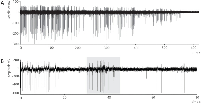
Figure 5: Representative extracellular recordings of swim pacemaker signals from the isolated rhopalium of Tripedalia cystophora. (A) Example of progressive electrode seal loss during an extended recording session. Pacemaker signal amplitude begins to decline at approximately 200–250 s, reflecting deteriorating electrical contact between the electrode tip and the epidermal stalk nerve, and the signal is completely lost by approximately 580–600 s. Both signal amplitude and background noise decrease in parallel, which is the characteristic signature of seal loss. (B) Representative recording of a visually evoked obstacle avoidance response above the DTT. The gray shaded area indicates the stimulus window, defined by the Arduino TTL signal, during which a high contrast (c = 0.80) vertical bar obstacle was moved across the full width of the lower lens eye visual field. Pacemaker signal frequency increases markedly during the stimulus window, consistent with a visually evoked obstacle avoidance response, and returns toward baseline frequency following stimulus offset. Spontaneous pacemaker signals occurring outside the stimulus window are expected and do not constitute visually evoked responses. Note that the difference in y-axis scale between panels reflects the different recording qualities shown and does not imply a difference in signal strength; in extracellular electrophysiology, signal amplitude depends on electrode seal quality rather than physiological response magnitude. All values are post-amplification (×1000). Please click here to view a larger version of this figure.

5. Rhopalium isolation and transfer

NOTE: This procedure is performed each time a rhopalium is required: once with a sacrificial rhopalium for the biological calibration in Section 4, and subsequently for each experimental rhopalium used in Section 6. On each occasion, all hardware must be fully assembled and verified before the animal is handled. The number of experimental rhopalia is determined by the experimental design.

1. Using a disposable plastic transfer pipette with the tip cut to yield an opening of approximately 8 mm diameter, transfer a single animal from the culture tank to a 35 mm Petri dish containing 0.20 µm filtered seawater from the culture tank.
2. Remove excess seawater until the animal is flattened against the dish and immobile, but not desiccated.
3. Using fine scissors (Vannas scissors, 0.025 mm × 0.015 mm blade), transect the stalk connecting the rhopalium to the bell at approximately two-thirds up the stalk length measured from rhopalial attachment (i.e., distal to the rhopalium). Immediately after transection, refill the Petri dish with 0.20 µm filtered seawater from the culture tank.
   CAUTION: Vannas scissors are extremely sharp. Handle with care during dissection to avoid injury.
   NOTE: The rhopalium may retract into the rhopalial niche following transection. Refilling the Petri dish with filtered seawater will, in most cases, dislodge the rhopalium. If not, use a Pasteur pipette to gently flush it out.
   Using a Pasteur pipette (150 mm), transfer the isolated rhopalium to the electrophysiology recording chamber positioned on the microscope stage. (CRITICAL) Ensure the rhopalium remains submerged in seawater at all times during and after transfer. Exposure to air will irreversibly damage the preparation.
4. Using a transfer pipette, return the animal to the culture tank.
   NOTE: Loss of a single rhopalium does not significantly impair normal box jellyfish behavior; animals retaining as few as one rhopalium continue to display normal feeding and light shaft interaction behaviors. Rhopalia additionally regenerate to full functionality, including restoration of pacemaker signaling and normal photoreceptor responses, within two weeks of removal²³. The animal may be used again in subsequent sessions until no rhopalia remain. Once all four rhopalia have been removed, the animal is no longer capable of generating swim pacemaker signals or bell contractions and is humanely disposed of via standard laboratory sink disposal, consistent with the disposal of rhopalium tissue (step 6.2.5).

6. Recording

1. Rhopalium positioning and electrode attachment
   1. Fill the recording suction electrode by drawing seawater directly from the recording chamber into the capillary until the internal solution reaches halfway up the silver wire. Fill the holding micropipette with sufficient seawater from the recording chamber to enable suction adhesion to the crystal.
   2. Mount the holding micropipette in a micromanipulator. Attach the tip of the holding micropipette to the calcium sulfate (CaSO₄) crystal at the distal end of the rhopalium by applying gentle suction via an attached Luer-lock syringe. The crystal provides a robust mechanical anchor point without damaging the neural tissue.
   3. Using the holding micropipette, position the rhopalium on the edge of the coverslip facing the projection screen (Figure 1D).
      NOTE: (CRITICAL) The distance between the lower lens eye and the projection screen must be measured and recorded, as it is required to calculate the angular subtense (acceptance angle) of projected image features at the lower lens eye using:
      
      ​where α is the visual angle, a is the width of the image feature, and b is the distance from the lower lens eye to the screen. At a working distance of 2 mm, a projected image of 16 mm × 12 mm (w × h) subtends approximately 150° horizontally and 120° vertically of the 170° circular visual field of the lower lens eye. The working distance must be kept constant across all recordings, as any deviation invalidates the angular calculations for the presented stimuli and prevents direct comparison across recordings.
   4. While maintaining rhopalium position with the holding micropipette, advance the recording electrode toward the transected surface of the stalk using a second micromanipulator.
      NOTE: The epidermal stalk nerve runs longitudinally through the full length of the stalk, from the rhopalial attachment point to the ring nerve¹⁵. On the transected surface, the nerve endings of the bifurcated epidermal stalk nerve are exposed and available for electrode contact on the adoral surface of the stalk — the side facing the lens eyes (Figure 2B).
   5. Apply gentle suction via Luer-lock syringe until a stable signal is established.
      NOTE: The nerve endings are not always visually distinguishable on the transected surface. Position the electrode tip over the region where the epidermal stalk nerve is expected based on anatomical landmarks and apply gentle suction. Adequate electrode attachment is indicated by the appearance of large, clearly resolved pacemaker signals with a consistent waveform at the expected frequency of 0.5–1 Hz (Figure 5). Pacemaker signals are distinguished from action potential-like signals on the basis of waveform duration and morphology (Figure 2C,D)^13,20,24. The appearance of stable pacemaker signals is the definitive criterion for correct electrode placement, not visual confirmation of nerve contact. If no signal is obtained, release suction, reposition the electrode tip slightly on the transected surface, and reapply. Excessive suction risks occluding the tip with tissue debris or mechanically damaging the nerve ending. Progressive loss of signal amplitude and background noise during recording is indicative of electrode seal loss (Figure 5A).
   6. Allow the preparation to acclimate for a minimum of 10 min following electrode attachment before commencing recordings. During this period, keep the projection screen illuminated with the white background and the gray bar positioned stationary to one side of the visual field, outside the center.
      NOTE: Before beginning acclimation, confirm preparation responsiveness by presenting a single maximum-contrast stimulus (c ≈ 1.0); rhopalia that do not respond are excluded from the dataset. The acclimation period allows the preparation to stabilize following the mechanical disturbance of electrode attachment. Maintaining the white screen with a stationary bar ensures that the photoreceptors are light-adapted to the baseline conditions that will prevail during visual stimulation, and that the initial pacemaker baseline frequency is stable before the first stimulus is presented. This is a further practical advantage of using presentation software for stimulus control. The screen content during acclimation and between recordings is directly visible and fully controllable without additional programming.
   7. Once a stable pacemaker signal is established, optimize the bandpass filter settings on the extracellular amplifier to maximize signal-to-noise ratio and preserve signal amplitude and waveform morphology, monitoring the effect on the oscilloscope display. Use the following starting settings: highpass 1 Hz and lowpass 500 Hz; engage the 50/60 Hz notch filter (EXT-10-2F integrated add-on). Adjust as needed based on the observed signal.
      NOTE: Raising the highpass cutoff above 1 Hz will progressively attenuate the low-frequency components of the pacemaker signal, reducing its amplitude and potentially compromising signal detection. The target post-amplification signal amplitude for clean, readily identifiable pacemaker signals is 400–600 mV, with a maximum of approximately 1 V.
2. Data acquisition
   1. Configure the VI (supplied as supplementary material, Supplementary File 3) to acquire the following channels simultaneously via the DAQ at a sampling rate of 1 kHz:
      Channel 1: Electrophysiological signal (amplified and filtered pacemaker signal from EXT-10-2F)
      Channel 2: LabVIEW-generated analog TTL output to the TTL mouse)
      Channel 3: Arduino Uno analog TTL timestamp (records the verified stimulus window — onset defined by TTL going high, termination defined by TTL returning low — as detected by the photodiode monitoring the black and white indicator square on the computer display).
      ​NOTE: Channel 2 records the intended stimulus delivery time, and Channel 3 records the verified actual stimulus window. Channel 3 should be used as the definitive stimulus timing record for all analyses.
   2. Set the recording duration according to the experimental protocol. For a standard stimulus presentation sequence consisting of a 30 s pre-stimulus baseline, approximately 15 s of visual stimulation, and a 35 s post-stimulus period, set the total recording duration to 80 s.
      NOTE: This protocol typically uses 10 biological replicates (rhopalia), preferably obtained from 10 different animals, to evaluate response strength, consistent with Bielecki et al. (2023)¹⁴. Within a single preparation, the same isolated rhopalium receives the entire visual stimulus protocol, presented sequentially from lowest to highest contrast; this order prevents the animal from habituating to an absence of aversive consequence at high contrast, which could otherwise reduce responsiveness to subsequently presented lower-contrast stimuli. Successive recordings are initiated at fixed 2-min intervals, yielding a 105 s interval between the end of one stimulus period and the onset of the next (sufficient for pacemaker frequency to return to baseline before the following stimulus). No technical replicates are performed; each rhopalium receives a single presentation per contrast level within its stimulus sequence.
   3. The LabVIEW VI (supplied as supplementary material, Supplementary File 3) automatically outputs a TTL pulse from the DAQ to the TTL mouse at the appropriate time point within the recording sequence, advancing the slide and initiating visual stimulus onset. Save the acquired data as a tab-delimited .txt file. When using the provided VI, recording metadata is encoded manually in the file name at the time of saving.
      NOTE: Users are encouraged to establish a consistent file naming convention prior to beginning recordings. A preparation identifier is a unique code (e.g., an animal or session number) that allows a given recording to be traced back to the specific rhopalium and experimental session from which it originated. The exact naming scheme is left to investigator preference, provided it is systematic and allows unambiguous retracing of any recording to its corresponding preparation — for example, a file name might combine the recording date and time with the relevant stimulus parameters (e.g., contrast level, bar dimensions, and speed).
   4. Following completion of all recordings for a given rhopalium, dispose of the rhopalium tissue via standard laboratory sink disposal.
      NOTE: Users are encouraged to establish a consistent file naming convention prior to beginning recordings. A systematic file name that includes date, preparation identifier, and stimulus condition is sufficient for downstream analysis. Presentation software is preferred over LabVIEW-generated visual stimuli for two practical reasons: first, it ensures that the image projected onto the lower lens eye between recordings is known and controlled at all times, preventing unintended visual stimulation from software interfaces or system screens; second, it eliminates the risk of screen blanking between recording sessions, which would elicit a light-OFF response in the photoreceptors and introduce spurious pacemaker activity into the subsequent baseline period. The perceived angular size and velocity of the bar will vary non-linearly across the visual field due to the geometry of the lens eye. This non-linearity is not corrected for two reasons: first, freely swimming animals do not approach obstacles with constant speed or direction, making angular correction of limited naturalistic relevance; second, correcting for angular size would require changes in overall screen luminance, which would engage the light ON/OFF response involved in detecting mangrove light shafts.

7. Data analysis

1. Pacemaker signal discrimination in Igor Pro
   NOTE: Swim pacemaker signals are discriminated from action potential-like signals in the raw electrophysiological trace prior to frequency analysis. The two signal types can occur simultaneously in the recording and must be distinguished before extracting pacemaker timing data. Representative examples of both signal types and their distinguishing waveform characteristics are provided in Figure 2C,D.
   1. Import the .txt data file into Igor Pro (version 6.37 or later) using the Neuromatic plugin (version 2.00).
   2. Discriminate swim pacemaker signals from action potential-like signals on the basis of signal duration and waveform morphology.
      NOTE: Swim pacemaker signals have a characteristic duration of approximately 45 ms and a compound waveform morphology reflecting the summed activity of multiple pacemaker neurons. Action potential-like signals have a shorter duration of approximately 10 ms and a sharper, unitary waveform. Signal amplitude alone is not a reliable discriminating criterion, as the two signal types can reach comparable amplitudes²⁴ (Figure 2C,D). A representative figure illustrating the distinguishing waveform characteristics of swim pacemaker signals and action potential-like signals is provided (Figure 2C,D). Users are encouraged to familiarise themselves with both signal types prior to analysis, as misidentification will introduce errors in pacemaker frequency estimation. Signal waveform characteristics are consistent within a given preparation but can vary somewhat between preparations; discrimination criteria should therefore be evaluated for each preparation individually, using the waveform characteristics described above as general guidance rather than fixed universal thresholds. For ambiguous or intermediate waveforms that cannot be confidently classified, resolve the ambiguity in the direction opposite to the expected or hypothesized outcome — for example, exclude an ambiguous event if a higher signal count would support the hypothesis being tested, or include it if a lower count would support it — to avoid inflating the apparent strength of the result.
   3. Extract the timestamp of each identified swim pacemaker signal to obtain a time series of pacemaker events for each recording, and export these timestamps (e.g., to a spreadsheet or .csv file) for downstream statistical analysis.
2. Frequency analysis
   1. Calculate the pacemaker signal frequency as the inverse of the inter-signal interval across the recording.
      1. Evaluate the effect of the visual stimulus by comparing pacemaker frequency during the pre-stimulus baseline period, the stimulus period, and the post-stimulus period, using pacemaker signal timestamps corrected for the delay between the LabVIEW-logged TTL command (Channel 2) and the Arduino-verified stimulus onset (Channel 3).
         NOTE: The lower lens eye responds to the stimulus on the timing of the verified TTL, not the software-logged command, so each recording's verified onset time is exported alongside the raw pacemaker and TTL timestamps to a spreadsheet (Supplementary Table 1) and used directly by the SAS analysis script to classify every pacemaker signal into its pre-stimulus, stimulus, or post-stimulus window (Figure 6); no timestamp values are modified at the spreadsheet stage. During undisturbed baseline conditions, the pacemaker signal frequency is 0.5–1 Hz. Visually evoked obstacle avoidance responses above the DTT are characterized by an increase in pacemaker frequency to 2–3 Hz. The physiological maximum is approximately 4 Hz, corresponding to a minimum inter-signal interval of 250–280 ms²⁵. Because baseline pacemaker frequency varies between preparations, frequency values for each recording are standardized relative to that recording's own mean frequency, calculated from the pre-stimulus and post-stimulus periods (excluding the stimulus period itself). This normalization allows response magnitude to be compared across preparations independent of differences in baseline pacemaker rate. Full statistical procedures for evaluating response significance, including the non-linear model used to compare baseline, stimulus, and post-stimulus periods, are described in Bielecki et al. (2023)¹⁴; the corresponding SAS analysis code is available at doi: 10.17632/csgymw8kjk.1. A representative analysis workflow, from raw signal through discrimination, frequency calculation, and standardization to the final response metric, is provided in Figure 7.

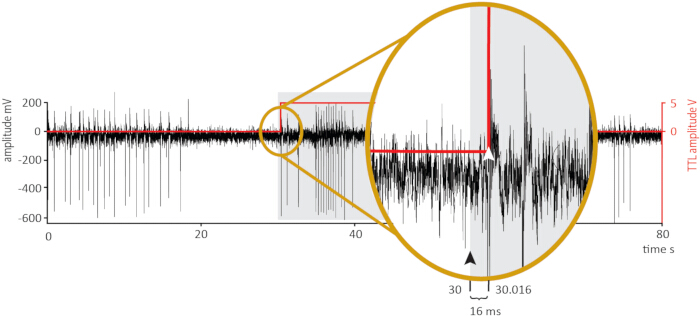
Figure 6: Representative demonstration of pacemaker timestamp correction for stimulus-verified timing. Example recording illustrating the delay between the VI-logged TTL command and the Arduino-verified stimulus onset, verified individually for each recording via the Arduino/photodiode timing chain and exported to a spreadsheet (Supplementary Table 1) for direct use by the SAS analysis script in classifying each pacemaker signal timestamp into its pre-stimulus, stimulus, or post-stimulus window. Black trace (left y-axis): electrophysiological signal (mV). Red trace (right y-axis): TTL amplitude (V). The gray shaded region marks the nominal stimulation window as timestamped by the software-logged TTL command. Inset: expanded view of the TTL onset. The black arrowhead marks the LabVIEW-logged TTL send time (t = 30.000 s, Channel 2); the white arrowhead marks the verified stimulus onset detected via the Arduino/photodiode chain (t = 30.016 s, Channel 3). The 16 ms interval shown is a representative example within the <20 ms range reported for automated TTL-mouse triggering (Results). Because this delay is constant within a given recording, the corresponding offset transition is not independently illustrated. Please click here to view a larger version of this figure.

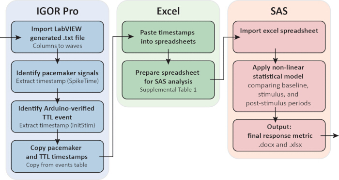
Figure 7: Representative analysis workflow, from raw recording to final response metric. Pacemaker signal and TTL timestamps are extracted from the Igor Pro/Neuromatic events table: pacemaker signal events are identified by duration, and waveform morphology (step 7.1.2), and the Arduino-verified stimulus onset (InitStim, Channel 3) is extracted for each recording as an absolute timestamp, not a calculated delay. These timestamps are copied to a spreadsheet (Supplementary Table 1), which is prepared for SAS analysis by computing the interspike interval (Intval) and midpoint timestamp (MidTime) for each pacemaker signal event. SAS imports the prepared spreadsheet and applies a non-linear statistical model (Bielecki et al., 2023¹⁴) comparing pacemaker frequency across the pre-stimulus, stimulus, and post-stimulus periods, classified relative to each recording's verified stimulus onset, to output the final response metric (.docx summary, .xlsx data tables). Please click here to view a larger version of this figure.

Results

Signal quality and spontaneous pacemaker activity

Following successful electrode attachment to the transected epidermal stalk nerve, spontaneous pacemaker signals should be immediately apparent on the oscilloscope. A high-quality recording is characterized by large, clearly resolved pacemaker signals of 400–600 mV post-amplification amplitude, occurring at a stable spontaneous frequency of 0.5–1 Hz, against a low-noise baseline (approximately 10–15 mV peak deviation on either side of zero, corresponding to a signal-to-noise ratio of approximately 27–40:1 within the target amplitude range) (Figure 5B). Recordings with signal amplitude as low as 100 mV can be analyzed, but substantially increase signal-discrimination time in Igor Pro and are not recommended, particularly for inexperienced operators. The compound waveform morphology of the pacemaker signal, reflecting the summed activity of multiple trmOC neurons, distinguishes it from the shorter, sharper action potential-like signals that may also be present in the recording²⁴ (Figure 2C,D). As described in step 7.1, these two signal types must be discriminated prior to analysis on the basis of signal duration (~45 ms for pacemaker signals versus ~10 ms for action potential-like signals) and waveform morphology. Amplitude alone is not a reliable discriminating criterion. Signal discrimination in this protocol was performed by a single, experienced operator; formal inter-rater reliability statistics were therefore not calculated (see Discussion, Limitations).

Visually evoked pacemaker response

In a healthy, responsive preparation, presentation of a moving vertical bar stimulus above the DTT to the lower lens eye produces a clear, time-locked pacemaker response. Pacemaker signal frequency increases to 2–3 Hz, coinciding with the passage of the leading edge of the obstacle across the center of the visual field, and returns toward baseline frequency after stimulus offset¹⁴ (Figure 5B). Stimulus onset timing was verified using the Arduino/photodiode timing chain (step 3.3) rather than relying on LabVIEW's own reported timestamp. Using the TTL mouse to advance the presentation software, the verified range is <20 ms; using manual triggering (an operator clicking an unmodified mouse timed to the desired onset), the verified range is 100–150 ms. Because response analysis uses the verified onset (Channel 3) rather than the software-reported trigger (Channel 2), this range does not affect response quantification regardless of the triggering method. This frequency increase constitutes the electrophysiological correlate of the obstacle avoidance behavior observed in freely swimming animals, and its presence confirms both the viability of the preparation and the correct optical alignment of the lower lens eye with the projection screen.

Pacemaker response magnitude is evaluated using instantaneous signal frequency, calculated as the inverse of the inter-signal interval between consecutive pacemaker events. This approach requires a minimum of two consecutive pacemaker signals to establish a frequency value, providing an inherent safeguard against false-positive response detection from single isolated signals.

The contrast of the moving bar stimulus determines the magnitude of the evoked response. In Bielecki et al. (2023)¹⁴, three contrast levels were used (c = 0.20, 0.40, and 0.80), spaced one f-stop apart. These specific contrast values were selected to keep the total protocol duration within the viable recording window of approximately 1 h. Researchers investigating the contrast sensitivity limits of the lower lens eye, or other specific visual response properties, should select contrast levels appropriate to their experimental question rather than adopting these values prescriptively.

Suboptimal recordings and failure modes

In practice, approximately 90% (9 of 10) of preparations meeting the acclimation viability criterion (step 6.1.6) go on to yield stable spontaneous activity and a measurable visually evoked response; this proportion is strongly dependent on operator experience. The remaining preparations most commonly fail for one of the following reasons: The most common failure mode is progressive loss of electrode seal during the recording session. This manifests as a gradual reduction in both pacemaker signal amplitude and background noise level, reflecting deteriorating electrical contact between the electrode tip and the nerve ending (Figure 5A). If this pattern is observed, suction should be released and reapplied after repositioning the electrode tip slightly on the transected stalk surface. If the signal amplitude does not recover, the preparation should be assessed for viability by checking for spontaneous pacemaker activity. Complete absence of signal following reattachment attempts, in a preparation that has been isolated for more than 1 h, most likely reflects preparation deterioration rather than electrode failure, and a fresh preparation should be used.

A second failure mode is the absence of a visually evoked response despite stable spontaneous pacemaker activity. This should prompt re-evaluation of the optical configuration before concluding that the preparation is unresponsive. The most common causes are misalignment of the lower lens eye relative to the projection screen and photoreceptor saturation from excessive irradiance. The biological calibration procedure described in step 4.1.5 should be repeated, and neutral density filter attenuation increased if necessary. It should also be verified that the moving bar stimulus remains within the visual field throughout its motion, as stimulus exit from the visual field would evoke a light-OFF response and introduce spurious pacemaker activity into the recording.

A third pattern — high background noise obscuring pacemaker signals — most commonly reflects a grounding problem or mains interference. The star grounding configuration described in step 3.2.1 should be verified, and the 50/60 Hz notch filter confirmed as engaged.

Supplementary File 1: Arduino sketch. Implements photodiode-based stimulus onset detection: the Arduino Uno samples the photodiode, monitoring the black-and-white indicator square on the presentation display (step 1.4.2) at 1 kHz, converts the raw analog signal to a clean digital TTL pulse via threshold comparison, and outputs this pulse as the verified stimulus timing signal (Channel 3, step 6.2.1).Please click here to download this file.

Supplementary File 2: Representative stimulus file. Example presentation-software file (Keynote) implementing the moving-bar visual stimulus as a single continuous object animation and the black-and-white timing-verification indicator square (step 1.4). Readers designing their own stimulus sequences should ensure the display remains stable for an adequate accommodation period before each stimulus onset; the photodiode/Arduino feedback loop (step 3.3) verifies true stimulus timing regardless of the specific presentation software or slide design used.Please click here to download this file.

Supplementary File 3: LabVIEW Virtual Instrument (VI). Configure the NI USB-6343 DAQ with two analog input channels — AI0 (electrophysiological signal from the amplifier) and AI1 (Arduino-verified stimulus-onset TTL, the photodiode feedback signal) — and one analog output channel, AO0, which delivers a TTL pulse to the TTL mouse at the programmed stimulus time to advance the presentation software slide. The resulting .txt output file records three columns: the electrophysiological signal (AI0), the LabVIEW-logged timestamp of the AO0 trigger command (a software record, not a re-acquired signal), and the Arduino-verified TTL (AI1).Please click here to download this file.

Supplementary Table 1: SAS input file format. Column definitions and a worked example for the spreadsheet uploaded to SAS for statistical analysis (step 7.2.1). Four consecutive pacemaker signal timestamps from a representative recording illustrate the derivation of the interspike interval (Intval) and midpoint timestamp (MidTime) used in frequency calculation; the final listed event has no Intval/MidTime value, since no subsequent timestamp exists to complete the interval.Please click here to download this file.

Discussion

Several steps in this protocol are critical to obtaining reliable recordings. The most consequential is the fabrication and preparation of the suction electrode. While any electrode that optimizes signal-to-noise ratio is acceptable for standard visually evoked pacemaker recordings, an attached resistance of approximately 1 MΩ becomes specifically critical when the preparation is used for delivery of an electrical unconditioned stimulus, as it is required to calculate the delivered current¹⁴. For recording purposes alone, the primary criterion is signal quality rather than a specific resistance value.

Equally critical is the biological calibration of the optical system prior to commencing recordings (step 4.1.5). Because projector output, lens configuration, and screen reflectance interact to determine the effective irradiance at the lower lens eye, no universally applicable irradiance value can be specified. The biological calibration (using the pacemaker frequency response to a maximum contrast stimulus as the criterion for photoreceptor dynamic range) provides a self-validating, hardware-independent method for establishing appropriate stimulus intensity. This step should not be omitted, as photoreceptor saturation from excessive irradiance will abolish visually evoked pacemaker responses and may be mistaken for a non-responsive preparation.

Maintaining rhopalium submersion throughout isolation and transfer is critical. The rhopalial nervous system is extremely sensitive to desiccation, and even brief air exposure can irreversibly damage the preparation. All transfer steps should be performed with seawater present, and the recording chamber should be filled with 0.20 µm filtered culture tank seawater before the rhopalium is introduced.

Finally, electrode placement on the transected stalk surface requires patience. The epidermal stalk nerve endings are not always visually identifiable, and correct placement must be confirmed by the appearance of spontaneous pacemaker signals on the oscilloscope.

The most common cause of recording failure is loss of electrode seal during the session. To minimize this risk, all protocols should be completed within one hour of rhopalium isolation. The one-hour limit recommended here is a conservative practical choice, reflecting the general expectation that an isolated neural preparation, disconnected from the rest of the animal, cannot be assumed to remain fully representative of intact physiological function indefinitely, even where pacemaker activity persists. Isolated rhopalia remain viable, in the sense of generating detectable pacemaker signals, for considerably longer than the recording window used in this protocol, up to approximately 5 h post-isolation; however, whether responses recorded late in this window remain fully representative of an intact preparation has not been systematically characterized, and the 1 h limit is used as a conservative buffer rather than a precisely defined threshold. Progressive loss of electrode seal is a separate, readily identifiable technical failure mode and the most common cause of signal loss within a single recording session (see below), but this does not rule out a contribution from preparation state to more subtle changes in responsiveness over time. If seal loss occurs during a recording, suction can be released, the electrode repositioned on the transected stalk surface, and suction reapplied. However, if the preparation has been isolated for more than one hour, it is advisable to begin a fresh preparation rather than invest time in troubleshooting a declining one.

Filter settings should be treated as starting points rather than fixed parameters. The bandpass filter values specified in this protocol (highpass 1 Hz, lowpass 500 Hz, 50/60 Hz notch) are those that optimize signal-to-noise ratio in the authors' recording environment. Laboratories with different levels of electrical interference, or using different amplifier models, may need to adjust these settings empirically on the amplifier controls while monitoring the signal on the oscilloscope display at the start of each session.

If spontaneous pacemaker activity is absent following electrode attachment, the preparation should be assessed before troubleshooting the electrode. A healthy isolated rhopalium will show spontaneous pacemaker signals at 0.5–1 Hz within minutes of electrode attachment. Absence of spontaneous activity most commonly reflects preparation damage during isolation or transfer rather than electrode failure. Conversely, if spontaneous activity is present but no visually evoked response is obtained, the optical calibration should be repeated before concluding that the preparation is unresponsive.

For laboratories adapting this protocol to different hardware, the TTL mouse and Arduino Uno timing verification chain described in step 3.3 can be replaced by any system that provides a hardware-level, software-independent stimulus window record acquired synchronously with the electrophysiological trace. The specific implementation described here was developed to bridge the LabVIEW acquisition environment on a PC with the presentation software on a separate computer, and reflects a practical engineering solution to a common cross-platform integration challenge. The underlying principle that software triggers alone are insufficient for precise stimulus-response timing analysis applies regardless of the specific hardware platform used.

The primary limitation of the isolated rhopalium preparation is that it records from a single rhopalium in isolation. In the intact animal, the four rhopalia are connected via the ring nerve¹⁵ and their outputs are integrated to produce coordinated swimming behavior. Inter-rhopalial communication is not accessible in this preparation. However, for the purpose of investigating visual information processing within a single rhopalial nervous system, this isolation is a strength rather than a weakness. It removes the confounding influence of inputs from other rhopalia and allows the visual response properties of a single RNS to be characterized in full.

Isolating the rhopalium also excludes multimodal sensory context beyond the rhopalium itself; the putative chemoreceptors anatomically described on its surface¹⁷ have not been functionally linked to the pacemaker response, so the signal can reasonably be interpreted as a readout of visual processing largely uncomplicated by non-visual input. A more fundamental limitation is that the extracellular stalk nerve recording captures only the integrated trmOC motor output signal. Individual subOC contributions to visual processing cannot be resolved electrophysiologically; this requires spatially resolved in vivo imaging approaches. The electrophysiological method described here is therefore a measure of the final integrated motor command, not of the intermediate processing steps within the RNS.

This has an important practical consequence: the isolated rhopalium electrophysiology protocol is not a standalone method. It is imperative that whole-animal behavioral analysis is performed prior to designing isolated rhopalium experiments, in order to establish which visual stimuli drive behaviors that alter bell contraction frequency. Behaviors that do not produce a change in pacemaker signal frequency cannot be assessed using this approach. The electrophysiological readout is specifically a measure of swim motor output, and experimental designs must be anchored in prior behavioral characterization to ensure that the chosen stimuli engage this output.

Recording success and signal classification both depend on operator experience. Approximately 90% of preparations meeting the acclimation viability criterion (step 6.1.6) yield stable spontaneous activity and a measurable visually evoked response in the hands of an experienced operator; this proportion is expected to be lower during the early stages of the learning curve. Signal discrimination between pacemaker and action potential-like waveforms (step 7.1.2) was performed by a single, experienced operator in this study; because formal inter-rater reliability testing requires multiple independent observers, it was not possible to calculate an inter-rater agreement statistic. Internal consistency was instead maintained by comparing ambiguous waveforms against a signal of known identity within the same recording, typically a maximum-contrast evoked response.

The hardware and software choices in this protocol — a modified projector lens, a custom TTL mouse, the Arduino timing chain, and LabVIEW/Igor Pro/SAS — reflect equipment and expertise already available in the authors' laboratory rather than a requirement of the method. The projector lens was modified because the standard configuration did not meet setup requirements. The TTL mouse bridges the stimulus computer and the acquisition computer: LabVIEW sends a TTL pulse to the mouse and logs the send time (Channel 2), and the mouse's click triggers the stimulus build via USB. Because the delay between this logged trigger and the actual screen change is variable, an independent photodiode/Arduino chain verifies true stimulus onset and feeds a second TTL back into the DAQ (Channel 3); a commercial alternative to the mouse may exist, but is unknown to the authors. None of this hardware requires specialized fabrication skill or high cost, and any substitute acquisition system needs only to meet the same 1 kHz synchronized multi-channel sampling requirement, plus whatever electronics or programming expertise that entails. With one exception: customizing a suitable analog amplifier requires expertise in low-noise circuit design not assumed of the reader.

T. cystophora combines the visual sophistication of genetically tractable systems such as Drosophila and zebrafish with the circuit-level tractability of numerically simple systems such as C. elegans: the rhopalial nervous system comprises approximately 1000 neurons, compared to on the order of 200,000 in the Drosophila brain¹ and 302 in the entire C. elegans nervous system². A further advantage of this system is its sensory hierarchy: T. cystophora possesses multiple sensory modalities, including mechanoreception (functionally implicated in associative learning¹⁴) and putative chemoreception (anatomically described but not functionally demonstrated¹⁷), in addition to vision. Within the isolated rhopalium preparation, however, only vision has been functionally demonstrated to drive the pacemaker response assessed by this protocol, allowing the signal to be interpreted as a comparatively unconfounded readout of visual processing, without the interpretive complication that arises when multiple concurrent active senses jointly shape a behavioral response. Visual stimuli can be specified with precision in space, time, and contrast, while the pacemaker signal can be used as a quantitative proxy for visually driven motor output, relevant to whole-animal behavior¹⁴.

Beyond visual electrophysiology, the isolated rhopalium preparation has been successfully applied to pharmacological investigation of the RNS through bath-applied neurotransmitter and neuromodulator assays, enabling identification of the transmitter systems that modulate pacemaker output²⁴. The preparation is also amenable to calcium and voltage imaging approaches. Preliminary unpublished work in the authors' laboratory, using a cell-permeant calcium indicator, supports the feasibility of calcium imaging in this preparation; voltage imaging remains untested. Such approaches could directly test the subOC–trmOC network architecture itself, which remains a working model, and would offer the spatial resolution needed to interrogate subOC and trmOC activity independently during visual stimulation, a capability that extracellular recording alone cannot provide. Together, these complementary approaches position the T. cystophora isolated rhopalium as a highly tractable preparation for systems-level investigation of visual processing and sensorimotor integration in a nervous system of defined and limited complexity.

Materials

List of materials used in this article

Name	Company	Catalog Number	Comments
35 mm Petri dish	Nunc	153066	Any equivalent petri dish suitable
Arduino Uno	Arduino	—	Converts photodiode signal to TTL for stimulus timing verification; 1 kHz refresh rate
Biconvex lens f = 30 mm	Linos	G063-022-000	Substituted for manufacturer lens; focuses image on projection screen wall of recording chamber
Borosilicate glass capillary tube, 1.16 mm ID × 2.00 mm OD × 80 mm L	Science Products	GB200-8P	For suction electrode fabrication
Disposable transfer pipette	Sarstedt	86.1171	Tip cut to ~8 mm opening for animal transfer
Electrode holder PPH-OP-BNCPC	ALA Scientific Instruments	PPH-OP-BNCPC	BNC-type holder with suction port; supplied with ~0.25 mm Ag wire
EXT-10-2F Extracellular Amplifier	NPI Electronic	—	Differential AC-coupled amplifier; headstage ×10, main amplifier ×100, total gain ×1000; integrated bandpass filter: highpass 1 Hz, lowpass 500 Hz; 50/60 Hz notch filter add-on engaged; supplied with headstage arm
Haemacytometer coverslip 20 mm × 26 mm	Carl Roth	L 189	Rests on coverslip ledges by negative buoyancy; more robust than standard coverslips
Igor Pro 6.37	WaveMetrics Inc.	Version 6.37	Lake Oswego, OR, USA; for pacemaker signal analysis
LabVIEW 2016	National Instruments	Version 2016	Acquisition and stimulus control software; VI supplied as supplementary material
Luer-lock syringe	—	—	Generic; any standard laboratory Luer-lock syringe suitable
Microforge MF-2	Narishige	—	For electrode tip polishing (Option A)
Micromanipulator MM33	Märzhäuser Wetzlar	00-42-101-0000 (right) / 00-42-102-0000 (left)	Manual three-axis; two required (holding pipette and recording electrode)
Micropipette puller, Flaming/Brown P-1000	Sutter Instrument	P-1000	Pulling program: Line 1×1: heat 535, pull 0, vel 12, time 200, pressure 600, ramp 540; Lines 2–4 × 3: heat 532, pull 0, vel 12, time 100
Neuromatic plugin v2.00	—	Version 2.00	For Igor Pro; pacemaker signal discrimination and timestamp extraction
Neutral density filter	Thorlabs	NE10A	10% transmission; attenuation to be validated empirically by biological calibration (step 4.1)
NI USB-6343 DAQ	National Instruments	781438-01	16-bit multifunction DAQ; electrophysiology acquisition, TTL mouse stimulus delivery, Arduino TTL input; sampling rate 1 kHz
Optoma ML750 DLP projector	Optoma	ML750	Manufacturer lens system removed; single biconvex lens f = 30 mm substituted
Oscilloscope DS1102E	Rigol	DS1102E	For real-time signal monitoring during electrode placement and filter optimisation
Pasteur pipette 150 mm	Carl Roth	4518	For rhopalium transfer
Photodiode BRW21	OSRAM	BRW21	Silicon photodiode; monitors black and white indicator square on computer display
SAS	SAS Institute Inc.	doi: 10.17632/csgymw8kjk.1	Cary, NC, USA; statistical analysis of pacemaker response; code available at doi: 10.17632/csgymw8kjk.1
Silicone tubing	Erich Eydam KG	9205000	For suction connection between electrode holder and syringe
Syringe filter Filtropur S, 0.20 µm PES	Sarstedt	83.1826.001	For filtering culture tank seawater for recording chamber and preparation dishes
Vannas scissors	World Precision Instruments	500086	0.025 mm × 0.015 mm blade; for rhopalial stalk transection
WTE var 3185	Assistent	—	Water bath temperature controller

References

- Raji JI, Potter CJ. The number of neurons in Drosophila and mosquito brains. PLoS ONE. 2021;16(5):e0250381.
- Sasakura H, Mori I. Behavioral plasticity, learning, and memory in C. elegans. Curr Opin Neurobiol. 2013;23(1):92-99.
- Bielecki J, et al. Pattern recognition in the box jellyfish rhopalial nervous system mimicked by an ensemble of pulsed coupled oscillators. Springer Series on Bio- and Neurosystems. Springer, Cham, 2024.
- Bielecki J, Garm A. Vision made easy: Cubozoans can advance our understanding of systems-level visual information processing. Marine organisms as model systems in biology and medicine. Springer, Cham, 2018.
- Nilsson D-E, Gislén L, Coates MM, Skogh C, Garm A. Advanced optics in a jellyfish eye. Nature. 2005;435(7039):201-205.
- Yatsu N. Notes on the physiology of Charybdea rastonii. J Coll Sci Imp Univ Tokyo. 1917;40:1-12.
- Bielecki J, et al. Ocular and extraocular expression of opsins in the rhopalium of Tripedalia cystophora (Cnidaria: Cubozoa). PLoS One. 2014;9(6):e98870.
- Plachetzki DC, Degnan BM, Oakley TH. The origins of novel protein interactions during animal opsin evolution. PLoS One. 2007;2(10):e1054.
- Koyanagi M, et al. Jellyfish vision starts with cAMP signaling mediated by opsin-Gs cascade. Proc Natl Acad Sci U S A. 2008;105(40):15576-15580.
- Kozmik Z, et al. Assembly of the cnidarian camera-type eye from vertebrate-like components. Proc Natl Acad Sci U S A. 2008;105(26):8989-8993.
- Garm A, Oskarsson M, Nilsson D-E. Box jellyfish use terrestrial visual cues for navigation. Curr Biol. 2011;21(9):798-803.
- Buskey E. Behavioral adaptations of the cubozoan medusa Tripedalia cystophora for feeding on copepod (Dioithona oculata) swarms. Mar Biol. 2003;142(2):225-232.
- Garm A, Mori S. Multiple photoreceptor systems control the swim pacemaker activity in box jellyfish. J Exp Biol. 2009;212(24):3951.
- Bielecki J, Dam Nielsen SK, Nachman G, Garm A. Associative learning in the box jellyfish Tripedalia cystophora. Curr Biol. 2023;33(19):4150-4159.e5.
- Garm A, Poussart Y, Parkefelt L, Ekström P, Nilsson D-E. The ring nerve of the box jellyfish Tripedalia cystophora. Cell Tissue Res. 2007;329(1):147-157.
- Garm A, Hedal I, Islin M, Gurska D. Pattern- and contrast-dependent visual response in the box jellyfish Tripedalia cystophora. J Exp Biol. 2013;216(24):4520-4529.
- Skogh C, Garm A, Nilsson D-E, Ekström P. Bilaterally symmetrical rhopalial nervous system of the box jellyfish Tripedalia cystophora. J Morphol. 2006;267(12):1391-1405.
- Nielsen SKD, Koch TL, Wiisbye SH, Grimmelikhuijzen CJP, Garm A. Neuropeptide expression in the box jellyfish Tripedalia cystophora—new insights into the complexity of a "simple" nervous system. J Comp Neurol. 2021;529(11):2865-2882.
- Satterlie RA, Spencer AN. Swimming control in a cubomedusan jellyfish. Nature. 1979;281(5727):141-142.
- Garm A, Bielecki J. Swim pacemakers in box jellyfish are modulated by the visual input. J Comp Physiol A. 2008;194(7):641.
- Govardovskii VI, Fyhrquist N, Reuter T, Kuzmin DG, Donner K. In search of the visual pigment template. Vis Neurosci. 2000;17(4):509-528.
- Garm A, Coates MM, Gad R, Seymour J, Nilsson D-E. The lens eyes of the box jellyfish Tripedalia cystophora and Chiropsalmus sp. are slow and color-blind. J Comp Physiol A. 2007;193(5):547-557.
- Stamatis S-A, Worsaae K, Garm A. Regeneration of the rhopalium and the rhopalial nervous system in the box jellyfish Tripedalia cystophora. Biol Bull. 2018;234(1):22-36.
- Bielecki J, Nachman G, Garm A. Swim pacemaker response to bath applied neurotransmitters in the cubozoan Tripedalia cystophora. J Comp Physiol A. 2013;199(9):785-797.
- Bielecki J, Høeg JT, Garm A. Fixational eye movements in the earliest stage of metazoan evolution. PLoS ONE. 2013;8(6):e66442.