A Reproducible Quantum-Classical Hybrid Protocol for Classifying Parkinson Disease from Human Voice Recordings

Summary

This protocol describes a reproducible quantum–classical hybrid workflow for classifying Parkinson Disease from human voice recordings, including data preprocessing, quantum circuit implementation, model training, and cross-validation for independent replication.

Abstract

Parkinson Disease is a progressive neurodegenerative disorder for which accessible, low-cost screening methods remain limited. Sustained-vowel voice recordings contain measurable acoustic biomarkers associated with disease-related dysphonia that can be acquired without specialized equipment. This protocol describes a four-qubit quantum–classical hybrid convolutional neural network (QI-HCNN) that combines a parameterized quantum circuit with a shallow classical classification layer to classify Parkinson Disease using dimensionally reduced acoustic voice features. The protocol also benchmarks the proposed approach against a dimensionality-matched classical neural network and gradient-boosted tree classifiers trained on both the reduced and full feature sets. Using a publicly available, de-identified dataset comprising 195 voice recordings from 31 individuals, the QI-HCNN achieved an area under the receiver operating characteristic curve of 0.78 using three-fold stratified cross-validation, compared with 0.87 for the matched classical neural network and 0.94–0.95 for the gradient-boosted baselines trained on the reduced and full feature sets, respectively. A controlled ablation analysis demonstrated that one of the two entanglement operations in the circuit could not influence the measured output by design, whereas the remaining entanglement operation reduced, rather than improved, classification performance relative to a non-entangled variant. Patient-grouped cross-validation further showed that performance estimates varied substantially depending on the individuals assigned to the test set, reflecting the limited cohort size. This protocol therefore provides a fully specified and independently reproducible quantum–classical baseline together with a data-supported evaluation of the strengths and limitations of the current circuit design, providing a methodological foundation for future investigations rather than supporting claims of diagnostic readiness.

Introduction

Parkinson Disease is a chronic neurodegenerative disorder caused by the progressive loss of dopaminergic neurons in the substantia nigra, affecting more than 10 million people worldwide and representing a substantial and growing public health burden¹. The disease produces both motor symptoms, including tremor, rigidity, and bradykinesia, and non-motor symptoms such as sleep disruption and anosmia. Clinical diagnosis relies primarily on neurological examination using standardized motor rating scales, supplemented, where available, by dopamine transporter imaging; however, both approaches require specialist expertise and infrastructure that are not uniformly accessible, and early-stage clinical assessment remains subjective². Because no disease-modifying therapy is currently available, early detection is valuable primarily because it enables earlier symptomatic management and longitudinal monitoring. This need has motivated the development of low-cost, scalable, and non-invasive screening approaches that can complement, rather than replace, clinical evaluation.

Vocal impairment is among the earliest measurable changes associated with Parkinson Disease and frequently precedes overt motor symptoms³. Sustained phonation of a held vowel provides a controlled signal from which acoustic features, including jitter, shimmer, harmonic-to-noise ratio, recurrence period density entropy, and detrended fluctuation analysis, can be extracted. These features have repeatedly been shown to contain diagnostically relevant information and can be acquired using consumer-grade recording equipment^4,5. A publicly available benchmark dataset derived from such recordings has become a standard testbed for this task, and classical machine-learning methods applied to the complete feature set, including support vector machines, random forests, and gradient-boosted trees, have reported area-under-the-receiver-operating-characteristic-curve values approaching 0.99^6,7,8, suggesting that the classification task is close to solved when the full feature set and appropriate strategies for handling class imbalance are used. Quantum machine learning has emerged as an alternative computational paradigm for biomedical classification tasks, in which parameterized quantum circuits use superposition and entanglement to represent feature interactions with comparatively few trainable parameters, and circuit gradients can be computed analytically using the parameter-shift rule rather than finite-difference approximations⁹. However, many published studies describing “quantum” or “quantum-inspired” neural networks for biomedical applications implement entirely classical architectures that adopt quantum-inspired mathematical formalisms without executing an actual parameterized quantum circuit on either a simulator or quantum hardware¹⁰. Recent developments in Parkinson Disease detection have also included hybrid convolutional neural network-transformer architectures¹¹, attention-based deep-learning methods for magnetic resonance imaging (MRI)¹², and lightweight convolutional neural networks designed for computationally efficient diagnosis¹³, illustrating the rapid expansion of artificial intelligence approaches across multiple data modalities. More broadly, non-invasive computer-aided diagnosis has been extended successfully to other biomedical applications, including hybrid machine-learning and deep-learning pipelines for medical imaging¹⁴. Comparative evaluations of deep-learning architectures on the same public voice dataset further demonstrate the strong performance achievable using conventional full-feature classical models¹⁵.

These developments highlight a specific methodological need for a reproducible quantum–classical hybrid convolutional neural network (QI-HCNN) model that (i) executes a genuine, fully specified parameterized quantum circuit; (ii) is benchmarked using identical input features against both an architecturally matched classical neural network and a strong classical baseline; and (iii) is evaluated using a protocol that explicitly examines the principal sources of bias in small biomedical datasets, including class imbalance, demographic confounding, and patient-level data leakage during cross-validation.

The overall goal of this protocol is to provide a fully reproducible QI-HCNN workflow for Parkinson Disease classification using human voice recordings. The protocol describes a four-qubit parameterized quantum circuit employing angle encoding, two controlled-NOT-based entanglement layers, and a trainable variational layer optimized using the parameter-shift rule, coupled with a shallow classical classification head and applied to a four-component principal-component representation of a publicly available voice-recording dataset. The workflow specifies, at a level sufficient for independent replication, all preprocessing procedures, complete circuit construction, classical training configuration, and evaluation procedures, including comparisons with a dimensionality-matched classical neural network, dimensionality-matched and full-feature gradient-boosted tree baselines, controlled circuit-component ablations, patient-grouped cross-validation to evaluate sensitivity to held-out participants, and explicit statistical significance testing. Rather than presenting only favorable outcomes, the protocol is designed to report transparently when individual circuit components do not measurably improve performance, thereby providing a reproducible methodological framework that can inform future QI-HCNN architecture development for small-cohort biomedical classification tasks.

Protocol

This protocol uses a publicly available, de-identified, third-party voice-recording dataset. No new human-subject data were collected by the authors, and no additional institutional review board (IRB) approval was required for this study. The dataset described in the Dataset Acquisition and Participant-Level Data Handling subsection was originally collected under institutional ethical approval by Little et al.³, contains no directly identifying participant information (only anonymized recording identifiers), and is publicly available for research use. Confirm, according to your institutional policies, whether secondary analysis of this publicly available dataset requires ethics review. At the authors' institution, retrospective secondary analysis of this fully de-identified, publicly archived dataset was determined to be exempt from full IRB review.

Dataset Acquisition and Participant-Level Data Handling
The Parkinson’s Disease Classification dataset (UCI Machine Learning Repository, Dataset ID 174), originally described by Little et al.³, was downloaded. The dataset contained 195 sustained-vowel /a/ phonation recordings from 31 individuals (23 diagnosed with Parkinson Disease and 8 healthy controls; age range, 46–85 years). Because the repository does not provide a versioned DOI, the exact download date was recorded and reported in the Table of Materials. The dataset was provided as a comma-separated values (CSV) file (parkinsons.csv). No decompression or file conversion was required, and the file was imported directly using the read_csv function from the Pandas library (see Table of Materials).

The downloaded dataset was verified to contain 195 rows and 24 columns comprising one recording identifier column (format: phon_R01_S subject _ recording), 22 continuous acoustic feature columns (Table 1), and one binary class-label column (status: 1 = Parkinson Disease; 0 = healthy control). Table 1 was used as the reference for all acoustic features and feature categories throughout the protocol.

Category	Representative Features	Clinical Significance
Fundamental frequency	MDVP:Fo(Hz), MDVP:Fhi(Hz), MDVP:Flo(Hz)	Average, maximum, and minimum fundamental frequency of phonation; reflects stability of vocal fold vibration.
Jitter (frequency perturbation)	MDVP:Jitter(%), MDVP:Jitter(Abs), MDVP:RAP, MDVP:PPQ, Jitter:DDP	Cycle-to-cycle variation in pitch period, reflecting impaired laryngeal motor control.
Shimmer (amplitude perturbation)	MDVP:Shimmer, MDVP:Shimmer(dB), Shimmer:APQ3, Shimmer:APQ5, MDVP:APQ, Shimmer:DDA	Cycle-to-cycle variation in signal amplitude, reflecting breathy or unstable phonation.
Noise measures	NHR, HNR	Ratio of noise to harmonic (tonal) components of the voice signal.
Nonlinear dynamics / fractal scaling	RPDE, D2, DFA, spread1, spread2, PPE	Measures of nonlinear vocal dynamics, periodicity, and long-range temporal correlations associated with vocal fold vibration.

Table 1: Acoustic feature categories used for Parkinson Disease classification. The 22 acoustic voice features extracted from the Parkinson's Disease Classification dataset are grouped into five feature categories: fundamental frequency, jitter, shimmer, noise measures, and nonlinear dynamics. Representative features are listed for each category together with their corresponding clinical significance. MDVP, Multidimensional Voice Program; RAP, relative average perturbation; PPQ, pitch period perturbation quotient; APQ, amplitude perturbation quotient; DDP, difference of differences of periods; DDA, average absolute difference of amplitudes; NHR, noise-to-harmonics ratio; HNR, harmonics-to-noise ratio; RPDE, recurrence period density entropy; D2, correlation dimension; DFA, detrended fluctuation analysis; PPE, pitch period entropy.

A participant identifier was extracted for each recording by parsing the substring preceding the final underscore in the recording name. For example, phon_R01_S01_1 and phon_R01_S01_2 were assigned to participant S01. Participant identifiers, rather than recording identifiers, were subsequently used for all grouped or leave-one-participant-out validation procedures described in the Evaluation Protocol subsection because recordings obtained from the same participant are acoustically correlated. After extraction, a frequency table of the identifiers was generated and inspected to confirm that all 195 recordings were assigned to exactly 31 unique participants, that no recording remained unassigned, and that the number of recordings per participant matched the source dataset documentation.

The class distribution was tabulated at both the recording level (147 Parkinson Disease recordings, 75.4%; 48 healthy-control recordings, 24.6%) and the participant level (23 of 31 participants, 74.2%, diagnosed with Parkinson Disease). Both distributions were reported because recording-level and participant-level class imbalance are not identical and influence downstream evaluation.

The absence of age- or sex-matched Parkinson Disease and healthy-control groups in the source dataset was documented as a study limitation and carried forward to the Discussion because this characteristic reflects the original data collection and cannot be corrected through downstream preprocessing.

Preprocessing Pipeline
All preprocessing procedures were performed independently within each training fold of the cross-validation procedure described in the Evaluation Protocol subsection. Both Min–Max normalization steps and principal component analysis (PCA) were fitted using only the training partition of each fold. The fitted transformations were subsequently applied to the corresponding held-out test partition without refitting to prevent information leakage from the test partition into the preprocessing parameters.

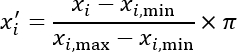
The 22 raw acoustic features in each training partition were normalized using a Min–Max scaler with an output range of [0, π]. The fitted scaler was then applied to both the training and test partitions of the corresponding fold (Equation 1). Equation 1 follows the standard Min–Max normalization formulation and was defined for the present protocol. Min–Max normalization was performed using the MinMaxScaler class from scikit-learn (version 1.8.0) with feature_range=(0, π), copy=True, and clip=False.

   (1)

A PCA model with n_components = 4 was fitted using only the normalized training data. The fitted PCA transformation was then applied to both the training and test partitions. The proportion of total variance explained by the four retained principal components was recorded for each fold. Across the analyses reported here, the four retained principal components explained 81.5% of the total variance (50.3%, 16.3%, 9.4%, and 5.5%, respectively). PCA was performed using the PCA class with n_components=4, svd_solver="full", whiten=False, and random_state=42.

Because PCA may generate negative-valued component scores, a second Min–Max scaler with an output range of [0, π] was fitted using the PCA-transformed training partition. The fitted scaler was subsequently applied to both the training and test partitions. Any transformed test-partition value that fell outside the interval [0, π] was clipped to the nearest boundary because the scaler had been fitted using only the training partition. No zero-variance features were present in the dataset. The range of every feature across all 195 recordings was strictly positive; therefore, no division-by-zero condition arose. This was confirmed by verifying that the scaled output contained neither NaN nor infinite values.

The four re-normalized principal components were assigned sequentially as rotation angles for qubits 0, 1, 2, and 3 during the angle-encoding procedure described in the Quantum Circuit Construction subsection. The first principal component was assigned to qubit 0, the second to qubit 1, the third to qubit 2, and the fourth to qubit 3. This completed the preprocessing pipeline and transferred the processed classical features to the quantum circuit. After the second Min–Max scaling step, all output values were confirmed to lie within the interval [0, π]. Test-partition values that fell marginally outside this range because of floating-point rounding were clipped to the nearest boundary using the clip function from NumPy (version 2.4.4). This procedure ensured that all four inputs to the angle-encoding layer were valid rotation angles within the interval [0, π].

Quantum Circuit Construction
The four-qubit circuit was constructed using the statevector simulator listed in the Table of Materials and the gate sequence described below. Supplementary Coding File 1 was used as the complete executable circuit implementation, including all helper functions for gate construction and parameter-shift gradient computation. Figure 1 shows the complete workflow from voice-recording preprocessing through the four circuit layers, the classical post-processing head, and final classification.

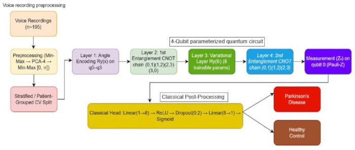
Figure 1. System architecture and quantum circuit workflow. Workflow for Parkinson Disease classification from human voice recordings. The diagram shows voice-recording preprocessing, stratified or patient-grouped cross-validation, four-qubit parameterized quantum circuit execution, single-qubit Pauli-Z measurement on qubit 0, classical post-processing, and final binary classification as Parkinson Disease or healthy control. CNOT, controlled-NOT gate; PCA, principal component analysis; ReLU, rectified linear unit. Please click here to view a larger version of this figure.

A four-qubit register was initialized in the computational basis state ∣0000.

For the angle-encoding layer, an R_y (x_i) rotation gate was applied to qubit i, where i = 0,1,2,3, using the four angles produced by the preprocessing pipeline (Equation 2). Equation 2 describes the standard angle-encoding procedure used in parameterized quantum circuits, consistent with the parameterized quantum circuit learning framework of Mitarai et al.⁹, and was applied here in the specific four-qubit configuration defined for the present protocol.

   (2)

For the first entanglement layer, a circular chain of controlled-NOT gates was applied in the following control-target order: (0,1), (1,2), (2,3), and (3,0).

For the variational layer, the eight trainable parameters w₀ through w₇ were initialized by independent sampling from a normal distribution with a mean of 0 and a standard deviation of 0.3. The random seed used was recorded in the Table of Materials. The eight variational quantum parameters were initialized using numpy.random.default_rng(42 + fold_index).normal(0, 0.3, size = 8), where fold_index is the zero-based fold number, thereby providing fold-specific but reproducible initializations. For each qubit i  = 0,1,2, and 3, an R_z(w_i) gate was applied, followed by an R_y(w_i+4) gate (Equation 3). Equation 3 describes a variational (trainable) quantum layer consistent with the general parameterized quantum circuit learning framework introduced by Mitarai et al.⁹ and was instantiated here using the specific gate sequence and parameterization defined for the present protocol.

(3)

For the second entanglement layer, an open chain of controlled-NOT gates was applied in the following control-target order: (0,1), (1,2), and (2,3). This chain was not closed back to qubit 0.

The expectation value of the Pauli- operator on qubit 0 only, , was computed using a statevector inner product. Circuit execution used a custom statevector simulator implemented using standard numerical array operations (Supplementary Coding File 1; qhcnn.py). Complex128 precision (numpy.complex128) was used throughout. Expectation values were computed analytically from the statevector inner product; therefore, no shot-based sampling was performed. No third-party quantum computing framework was required. If a sampling-based simulator or quantum device had been used instead of the statevector simulator, repeated computational-basis measurements of qubit 0 would have been performed, and the resulting bit frequencies would have been converted to an expectation value (Equation 4). Equation 4 is the standard quantum-mechanical expectation-value formula and was applied here to the single-qubit Pauli- observable defined for the present protocol. Because no shot-based sampling was performed, no measurement-error mitigation was required. The simulator used big-endian qubit indexing, with qubit 0 corresponding to the most significant bit of the statevector index. This convention was explicitly accounted for when constructing the Pauli- observable to ensure that the correct expectation value was measured.

(4)

The gradient of with respect to each of the eight variational parameters was computed using the parameter-shift rule. The circuit was evaluated twice for each parameter during every gradient computation, once at θ + π/2 and once at θ - π/2 (Equation 5). Equation 5 is the standard parameter-shift rule introduced by Mitarai et al.⁹ and was applied here without modification.

(5)

The second entanglement layer, as specified above, never applied a controlled-NOT gate with qubit 0 as the target. Because a controlled-NOT gate leaves the reduced state of its control qubit unchanged, the second entanglement layer could not alter , regardless of the trainable parameter values. To allow the second entanglement layer to influence the measured output in a modified protocol, qubit 0 would need to be included as a target, for example by closing the chain with an additional (3,0) controlled-NOT gate, or a multiqubit observable would need to be measured rather than a single-qubit expectation value. The originally specified second entanglement layer was retained in this protocol, and its measured contribution was reported explicitly in the Results section rather than corrected silently because this circuit behavior is part of the present findings.

Classical Post-Processing Layer
The classical post-processing stage consisted of a feed-forward neural network implemented using the standard array-based numerical operations listed in the Table of Materials. The single scalar circuit output, , was mapped to eight hidden units using a fully connected layer, followed by a rectified linear unit (ReLU) activation. During training, a dropout layer with a retention probability of 0.8 (dropout rate = 0.2) was applied. The eight hidden units were then mapped to a single output unit using a second fully connected layer, and a sigmoid activation function was applied to generate the final class probability, ŷ (Equation 6). Equation 6 defines the specific classical post-processing architecture used in the present protocol and comprises standard linear, rectified linear unit (ReLU), and sigmoid operations.

(6)

The first-layer and second-layer weight matrices were initialized by independent sampling from a normal distribution with a mean of 0 and a standard deviation of 0.5, whereas all bias terms were initialized to 0. The same random-number-generator instance and seed used for initialization of the quantum variational parameters were also used for the classical layer to ensure run-to-run reproducibility. Specifically, the classical weight matrices were initialized using numpy.random.default_rng(42 + fold_index).normal(0, 0.5, size=...), whereas all bias terms were initialized to zero. A single seeded random-number-generator instance, initialized with 42 + fold_index, was created at the start of each cross-validation fold and reused sequentially for quantum-parameter initialization, classical-weight initialization, mini-batch shuffling, and dropout-mask generation, rather than using separate independent seed streams for each process.

During training, dropout was applied by generating a newly sampled binary mask at each forward pass using the inverted-dropout convention, in which surviving units were scaled by 1/0.8. During validation and testing, dropout was disabled completely, and the full, unscaled network was used for inference.

The combined QI-HCNN model contained 33 trainable parameters: eight quantum variational parameters from the quantum circuit and 25 classical parameters. The classical component comprised eight weights and eight biases in the first fully connected layer, together with eight weights and one bias in the second fully connected layer. The weight and bias tensor dimensions were and . The classical post-processing layer was implemented entirely using standard numerical array operations without an additional machine-learning framework. All classical computations were performed using float64 (double-precision) arithmetic.

Model Training
The quantum circuit described in the Quantum Circuit Construction subsection and the classical post-processing layer described in the Classical Post-Processing Layer subsection were combined into a single end-to-end trainable model. All 33 trainable parameters were optimized jointly using the Adam optimizer with an initial learning rate of 0.01 and weight decay, implemented as an L2 penalty of , applied only to the classical weight matrices. The Adam optimizer was implemented manually using standard numerical array operations with the following settings: learning rate = 0.01, β₁ = 0.9, β₂ = 0.999, ∈ = 1 × 10^-8, and weight decay = 1 × 10^-4, applied only to the classical weight matrices and not to the bias terms or quantum variational parameters.

Binary cross-entropy was used as the loss function. For the post-split class-balancing procedure described in the Evaluation Protocol subsection, each training sample's loss contribution was weighted by the inverse frequency of its class within the training partition of the current fold. For the unbalanced protocol, uniform sample weights were assigned. Binary cross-entropy was computed as the mean loss across all samples within each mini-batch using the standard binary cross-entropy formulation.

The model was trained for 30 epochs using mini-batches of 16 samples. Training samples were randomly shuffled at the start of each epoch using numpy.random.default_rng(42 + fold_index).permutation(n) to generate a random sample order. When the number of training samples was not evenly divisible by 16, the final smaller mini-batch was retained and processed at its actual size rather than discarded.

A step learning-rate schedule was applied during training. The learning rate was multiplied by 0.7 after every 10 completed epochs, specifically at the start of epochs 11 and 21.

Gradients for the eight quantum variational parameters were computed using the parameter-shift rule described in the Quantum Circuit Construction subsection. Gradients for the 25 classical parameters were computed using standard reverse-mode differentiation through the classical layer only. The quantum circuit output, , and its parameter-shift gradients served as the interface between the quantum circuit and the classical layer. All 33 parameters were updated using the same Adam optimizer instance.

Validation-based early stopping was not used. Each model was trained for the fixed 30-epoch schedule, and held-out test-partition performance was reported after completion of the final epoch. All model parameters (quantum variational parameters, classical weight matrices, and bias terms) were reinitialized independently at the start of each cross-validation fold using the fold-specific random seed (42 + fold_index). Parameters were not shared across folds or baseline runs.

The computational environment, including processor, memory, software versions, and approximate wall-clock training time per fold, was recorded in the Table of Materials.

Evaluation Protocol
Model performance was evaluated using both recording-level and participant-level cross-validation procedures, together with baseline-model comparisons, class-balancing analyses, circuit ablation experiments, statistical significance testing, and feature-importance analyses.

For the primary evaluation, the 195 voice recordings were partitioned into three stratified folds using a fixed random seed while preserving the recording-level Parkinson Disease/healthy-control ratio of 75.4%/24.6% within each fold. The model described in the preceding sections was trained using two folds and evaluated on the remaining held-out fold, and this procedure was repeated until each fold had served once as the test partition. Accuracy, precision, recall, F1-score, and area under the receiver operating characteristic curve (AUC–ROC) were calculated for each fold and reported as the mean ± standard deviation across the three folds. Primary three-fold stratified cross-validation was implemented using the StratifiedKFold class with n_splits=3, shuffle=True, and random_state=42.

Binary class predictions were generated by applying a fixed probability threshold of 0.50 to the predicted class probability, ŷ, produced by the classical post-processing layer. Accuracy, precision, recall, and F1-score were computed from these thresholded predictions, whereas AUC–ROC was calculated directly from the continuous probability values without thresholding. Precision, recall, and F1-score were computed using the metric functions with zero_division=0, assigning a value of 0.0 to any undefined metric. No such undefined condition occurred during the reported experiments.

Baseline models were evaluated using the identical fold partitions and identical four-component preprocessed feature representation generated by the preprocessing pipeline. A classical multilayer perceptron containing one hidden layer of eight ReLU-activated units, architecturally matched to the classical component of the hybrid model but without the quantum circuit, was trained using the Adam optimizer with an L2 penalty of 1 × 10⁻⁴. A gradient-boosted tree classifier was also trained using the same four-component representation with 200 trees, a maximum tree depth of 3, a learning rate of 0.1, and class weighting equal to the inverse class frequency within each training fold. In addition, a second gradient-boosted tree classifier was trained using the full 22-feature representation generated after the initial Min–Max normalization, without applying PCA or quantum feature encoding. This model used 300 trees, a maximum tree depth of 4, a learning rate of 0.05, and the same inverse training-fold class-weighting strategy. The classical multilayer perceptron baseline was implemented using MLPClassifier with hidden_layer_sizes=(8,), activation="relu", solver="adam", alpha=1 × 10⁻⁴, batch_size="auto", learning_rate_init=0.001, max_iter=500, early_stopping=False, shuffle=True, and random_state=42. The default Glorot (Xavier) uniform weight initialization provided by the implementation was used. The gradient-boosted tree baselines were implemented using XGBoost 3.3.0 with objective = "binary:logistic", eval_metric = "logloss", tree_method = "auto", subsample = 1.0, colsample_bytree = 1.0, reg_alpha = 0, reg_lambda = 1, and random_state = 42.

To evaluate the effect of post-split class balancing, the primary cross-validation procedure was repeated for the QI-HCNN model with sample weighting enabled. Balancing weights were calculated exclusively from the training partition of each fold after train/test splitting and were not computed from the corresponding held-out test partition.

Circuit-component ablation experiments were performed by repeating the complete preprocessing, training, and evaluation workflow four times while modifying only the two entanglement layers of the quantum circuit. The four circuit variants comprised: (i) the complete circuit containing both entanglement layers; (ii) the circuit with the first entanglement layer removed and the second retained; (iii) the circuit with the first entanglement layer retained and the second removed; and (iv) the circuit with both entanglement layers removed. Identical fold partitions, random seeds, and training configurations were maintained across all four experiments so that any observed performance differences could be attributed solely to the entanglement-layer configuration.

As a robustness assessment, participant-grouped cross-validation was performed by partitioning the 31 participants, rather than the 195 recordings, into five groups containing six to seven participants each. During each iteration, the model was trained using recordings from participants in four groups and evaluated using recordings from participants in the remaining group, ensuring that no participant contributed recordings to both the training and test partitions of the same fold. Accuracy, precision, recall, F1-score, and AUC–ROC were reported as the mean ± standard deviation across the five participant-grouped folds for the QI-HCNN model, the classical multilayer perceptron, and the four-feature gradient-boosted baseline. Participant-grouped cross-validation was implemented using the GroupKFold class with n_splits=5, where the participant identifiers served as the grouping variable. Because GroupKFold does not shuffle the groups, participants were assigned according to the implementation's default deterministic ordering, resulting in folds containing six or seven participants each.

Statistical significance was evaluated by applying paired Wilcoxon signed-rank tests to the per-fold AUC–ROC values obtained for the primary evaluation and baseline models. Exact p-values and the corresponding numbers of paired observations were reported because the statistical power of this test is limited when only a small number of folds are available. Four pairwise AUC–ROC comparisons were defined a priori: (1) QI-HCNN versus the classical multilayer perceptron; (2) QI-HCNN versus the PCA-matched gradient-boosted tree baseline; (3) the classical multilayer perceptron versus the PCA-matched gradient-boosted tree baseline; and (4) the unbalanced QI-HCNN model versus the post-split-balanced QI-HCNN model. No multiple-comparison correction was applied because the analyses were exploratory and the limited number of folds substantially reduced statistical power.

Feature-importance analysis was performed using the gradient-boosted tree classifier trained on the complete 22-feature representation. Gain-based feature-importance scores were extracted and ranked for all original acoustic features. Separately, PCA was fitted to the complete dataset for reporting purposes only and was not used during model evaluation. For each original acoustic feature, the absolute loadings across the four retained principal components were summed, and features were ranked according to these values. Both ranking methods and their overlap were reported. For the gain-based feature-importance analysis, the gradient-boosted tree implementation produced unique floating-point gain values, and no ties occurred. For the principal-component loading rankings, ties in the summed absolute loading values were resolved according to the original feature-column order in the dataset.

Results

All numerical values reported in the text are reconciled with, and identical to, those presented in Figures 2–8 and Tables 2–4. Every figure was generated directly from the code provided in Supplementary Coding File 1 rather than manually prepared, ensuring consistency between the reported numerical values and the plotted data.

Primary Cross-Validation Performance
Under the unbalanced training protocol, the QI-HCNN model a...

Discussion

This protocol specifies a fully reproducible QI-HCNN architecture for Parkinson disease classification from voice recordings, in which every gate, parameter-initialization choice, preprocessing step, and evaluation procedure is described at a level sufficient for independent implementation. The proposed circuit is benchmarked using identical input features and identical cross-validation fold partitions against an architecturally matched classical multilayer perceptron and gradient-boosted tree baselines. This benchmarkin...

Materials

List of materials used in this article

Name	Company	Catalog Number	Comments
Adam optimizer	Standard numerical-optimization implementation	Custom implementation; NumPy 2.4.4	Joint optimization of quantum and classical parameters; Model Training
Binary cross-entropy loss implementation	Custom implementation using NumPy	NumPy 2.4.4; loss averaged (mean reduction) across each mini-batch	Training loss function; Model Training
Gradient-boosted tree classifier	XGBoost open-source gradient-boosting library	XGBoost 3.3.0; objective="binary:logistic"; eval_metric="logloss"; tree_method="auto"; random_state=42	PCA-matched and full-feature classical baselines; Evaluation Protocol
Machine-learning library	scikit-learn open-source machine-learning library	scikit-learn 1.8.0	Min–Max scaling, principal component analysis, stratified cross-validation, participant-grouped cross-validation, multilayer perceptron baseline, and evaluation metrics
Numerical computing library	NumPy open-source numerical computing library	NumPy 2.4.4	Core array operations, statevector simulation, parameter initialization, and manual gradient computation
Parkinson’s Disease Classification dataset	Little, McSharry, Roberts, Costello, and Moroz; distributed through the UCI Machine Learning Repository	UCI Dataset ID 174; 195 recordings from 31 participants; accessed June 19, 2025	Source sustained-vowel voice-recording dataset; https://archive.ics.uci.edu/dataset/174
Scientific computing library	SciPy open-source scientific-computing library	SciPy 1.17.1	Wilcoxon signed-rank statistical significance testing; Evaluation Protocol
Statevector simulator	Custom statevector simulator (Supplementary Coding File 1; qhcnn.py)	Pure NumPy implementation; complex128 (double) precision; no external backend required	Execution of the four-qubit quantum circuit; Quantum Circuit Construction
Tabular data library	Pandas open-source data-analysis library	Pandas 3.0.2	Dataset loading, inspection, and tabular manipulation
Workstation computational environment	Local CPU workstation (cloud-hosted Linux container)	x86_64 CPU; Ubuntu Linux; Python 3; no GPU or quantum hardware used; approximate wall-clock training time of 30–60 seconds per fold	Computational environment used for all training and evaluation; CPU-based statevector simulation; no GPU or quantum hardware required

References

- Rabie H, Akhloufi MA. A review of machine learning and deep learning for Parkinson's disease detection. Discov Artif Intell. 2025;5:24.
- Devi SVA, et al. Hybrid deep learning methods for enhancing Parkinson's disease early detection [conference presentation]. Presented at: 4th International Conference on Smart Applications, Data and Living (ICSADL); 2025; Bhimdatta, Nepal. IEEE. p. 1462-1469. Available from: https://doi.org/10.1109/ICSADL65848.2025.10933259.
- Little MA, et al. Exploiting nonlinear recurrence and fractal scaling properties for voice disorder detection. Biomed Eng Online. 2007;6:23.
- Costantini G, et al. Artificial intelligence-based voice assessment of patients with Parkinson's disease off and on treatment. Sensors (Basel). 2023;23(4):2293.
- Gunduz H. Deep learning-based Parkinson's disease classification using vocal feature sets. IEEE Access. 2019;7:115540-115551.
- Naeem I, et al. Voice biomarkers as prognostic indicators for Parkinson's disease using machine learning techniques. Sci Rep. 2025;15:12129.
- Ebrahimzadeh E, et al. Explainable machine learning for early detection of Parkinson's disease in aging populations using vocal biomarkers. Front Aging Neurosci. 2025;17:1672971.
- Alishah S. An explainable ensemble and deep learning framework for accurate and interpretable Parkinson's disease detection from voice biomarkers. Diagnostics (Basel). 2025;15(22):2892.
- Mitarai K, Negoro M, Kitagawa M, Fujii K. Quantum circuit learning. Phys Rev A. 2018;98(3):032309.
- Alissa M, et al. Parkinson's disease diagnosis using convolutional neural networks and figure-copying tasks. Neural Comput Appl. 2022;34(2):1433-1453.
- Kumari GRP, Ravi Kanth M, Kamal MV. Parkinson's disease early detection using hybrid attentive CNN-transformer model. Neural Comput Appl. 2025;37(32):26523-26543.
- Palakayala R, Kuppusamy P. AttentionLUNet: a hybrid model for Parkinson's disease detection using MRI brain. IEEE Access. 2024;12:91752-91769.
- Wang X, et al. A light-weight CNN model for efficient Parkinson's disease diagnostics [conference presentation]. Presented at: IEEE International Symposium on Computer-Based Medical Systems (CBMS); 2023; L'Aquila, Italy. IEEE. p. 616-621. Available from: https://doi.org/10.1109/CBMS58004.2023.00289.
- Haq I, et al. Lung nodules localization and report analysis from computerized tomography (CT) scan using a novel machine learning approach. Appl Sci. 2022;12(24):12614.
- Alzaidi A, et al. Comparative study of deep learning models for Parkinson's disease detection using the UCI vocal dataset. TBench. 2025;5(2):10021
Access restricted. Please log in or start a trial to view this content.