Multi-view Vision Mamba U-Shaped Network Framework for Medical Image Segmentation

Summary

This protocol describes how to construct, train, and evaluate a multiview Vision Mamba U-Shaped Network framework for medical image segmentation, enabling reproducible segmentation of skin lesions and abdominal organs through standardized dataset preparation, model implementation, and performance evaluation.

Abstract

Medical image segmentation requires computational methods that accurately capture global context, local boundaries, and multiscale anatomical structures while remaining reproducible across different applications. This article presents a protocol for constructing, training, and evaluating a Multi-view Vision Mamba U-Shaped Network framework for two-dimensional medical image segmentation. The protocol provides a reproducible workflow that includes public dataset acquisition, image and mask preprocessing, network construction, model training, checkpoint selection, and quantitative and qualitative performance evaluation. The framework incorporates multiview feature scanning to capture complementary spatial, contour, scale, and boundary information and applies multistage feature fusion within a U-shaped encoder-decoder architecture to improve feature integration during segmentation. The protocol is demonstrated using publicly available skin lesion and abdominal organ segmentation datasets. Under the described implementation workflow, the framework achieves competitive segmentation performance using standard evaluation metrics. By following the procedures presented in this protocol, researchers can reproduce the model implementation, train the network using defined experimental settings, evaluate segmentation performance, and adapt the workflow for related medical image segmentation tasks requiring reproducible deep learning–based analysis.

Introduction

Medical image segmentation is a fundamental task in the fields of computer vision and medical image analysis^1,2,3. It involves partitioning an image into multiple regions or objects for further analysis and processing. This technology is particularly important in medical imaging because it assists clinicians in identifying and localizing pathological regions, thereby improving diagnostic accuracy and treatment planning. With the advancement of medical imaging technologies, such as magnetic resonance imaging (MRI), computed tomography (CT), and positron emission tomography (PET), the demand for accurate medical image segmentation techniques has continued to increase. Current methods for medical image segmentation can be broadly categorized into three main approaches: convolutional neural network (CNN)-based methods⁴, Transformer-based methods⁵, and state-space model (SSM)-based methods^6,7. CNN-based methods typically employ U-shaped network architectures for medical image segmentation. The most widely used architecture in this category is U-Net⁸, which demonstrated the effectiveness of a U-shaped encoder–decoder architecture for biomedical image segmentation. U-Net3+ combines dense skip connections from UNet++⁹ with full-scale skip connections to enhance multiscale feature aggregation. However, CNN-based methods have limited ability to capture long-range dependencies and, therefore, may not effectively model long-range contextual information.

Transformer-based methods effectively capture long-range dependencies through the self-attention mechanism, which enables parallel computation and assigns different attention weights to different regions of interest. UNETR++¹⁰ introduces the Efficient Paired Attention (EPA) module to reduce the number of parameters and computational cost. nnFormer¹¹ combines interleaved convolutional and self-attention operations and introduces a local–global volume-based self-attention mechanism for learning volumetric representations in three-dimensional (3D) medical image segmentation. H2Former¹² proposes an efficient hierarchical hybrid Vision Transformer that combines attention mechanisms with CNN-based feature extraction in the encoder. However, Transformer-based methods exhibit quadratic computational complexity with increasing sequence length, resulting in substantially higher computational cost. Figure 1 illustrates the motivation for MVM-UNet and compares the proposed multiview scanning strategy with existing SSM-based segmentation frameworks.

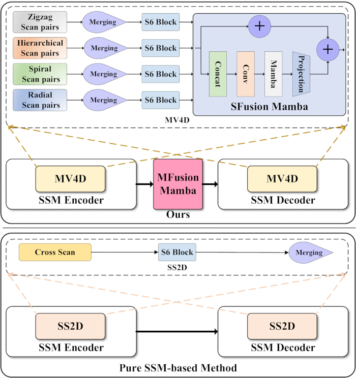
Figure 1. Comparison of MVM-UNet with existing pure state-space-model (SSM)-based segmentation architectures. Comparison between a conventional pure state-space model (SSM)-based segmentation framework and the proposed Multi-View Mamba U-Net (MVM-UNet) architecture. The upper panel illustrates MVM-UNet, in which the Multi-View 4-Directional (MV4D) module extracts complementary features using zigzag, hierarchical, spiral, and radial scan pairs that are integrated by Spatial Fusion Mamba (SFusion Mamba), while Multistage Fusion Mamba (MFusion Mamba) aggregates multiscale encoder features before decoding. The lower panel shows a representative pure SSM-based architecture using Selective Scan 2-Dimensional (SS2D) modules with cross scanning. The figure highlights the architectural differences between conventional SSM-based segmentation networks and the proposed MVM-UNet. Please click here to view a larger version of this figure.

SSM-based methods combine the global modeling capability of Transformers with linear computational complexity. The Mamba architecture selectively processes input information using a selective state-space model (Selective-SSM), enabling the model to dynamically adjust its parameters according to the input while filtering irrelevant information and emphasizing informative features. Vim¹³ and VMamba¹⁴ adapt the Mamba architecture for computer vision tasks. U-Mamba¹⁵ employs a hybrid CNN–SSM architecture to explore the application of SSMs in medical image segmentation, whereas Mamba-UNet¹⁶ adopts a fully SSM-based encoder–decoder architecture for medical image segmentation. These methods achieve competitive performance while using substantially fewer parameters. However, current SSM/Mamba-based methods primarily extract image features using simple image patches and SS2D scanning strategies, which present several limitations for medical image segmentation. First, SS2D and patch-based techniques are primarily designed for general computer vision tasks. Local Mamba¹⁷ and Motion Mamba¹⁸ have suggested that the SS2D scanning strategy is insufficient for all visual tasks because different scanning strategies capture different types of visual information. Second, the SS2D scanning strategy is relatively simple, relying only on horizontal and vertical scanning directions. Consequently, it may not adequately capture complex spatial relationships and fine structural details. Medical image segmentation requires simultaneous modeling of both global spatial context and precise local anatomical features. Furthermore, current SSM/Mamba-based methods provide limited feature fusion between the encoder and decoder. Architectures such as UNet++ and FATNet improve segmentation accuracy through enhanced feature fusion, highlighting the importance of effective feature integration for medical image segmentation.

To address these limitations, this paper proposes a novel Mamba-based medical image segmentation framework, termed MVM-UNet. As shown in Figure 1, the proposed Multi-View Four-Directional (MV4D) module serves as the core feature extraction component of MVM-UNet and is specifically designed for medical image segmentation by integrating information from four distinct scanning strategies. Each scanning strategy extracts complementary image features and represents a different view of the input image. Zigzag scanning¹⁹ alternates the traversal direction at the end of each row or column, thereby balancing local and global spatial information. In contrast, spiral and radial scanning schemes²⁰ provide comprehensive coverage by extending either outward from the center or inward from the periphery. Hierarchical scanning¹⁸ captures both local and global features at multiple scales. To improve the robustness of each scanning strategy, scan pairs are merged before being input to the S6 Block. The Scan-view Fusion Mamba (SFusion Mamba) module subsequently integrates the features extracted from the four scanning modalities. To effectively utilize multiscale encoder features, this paper further proposes a multiscale Mamba fusion module (MFusion Mamba), which accumulates and fuses the outputs from each encoder stage before passing the fused features to the decoder. MVM-UNet was evaluated on the ISIC 2017, ISIC 2018, and Synapse datasets. Experimental results demonstrate that MVM-UNet achieves competitive segmentation performance on the ISIC 2017, ISIC 2018, and Synapse datasets.

Representative segmentation architectures have further advanced medical image segmentation. U-Net has also been successfully applied to biomedical image analysis tasks such as cell counting, detection, and morphometry²¹. Attention-enhanced CNN architectures, such as CA-Net²², improve feature representation through comprehensive attention mechanisms. Representative Transformer-based segmentation frameworks, including TransUNet²³, Pyramid Medical Transformer²⁴, Swin U-Net²⁵, TransAttUNet²⁶, and TransCUNet²⁷, further demonstrate the effectiveness of attention-based global feature modeling for medical image segmentation.

The design of MVM-UNet is motivated by two limitations of existing SSM/Mamba-based segmentation methods. First, many current Vision Mamba models rely on simple two-dimensional scanning strategies, which may be insufficient for medical images containing irregular lesion boundaries, small target regions, and multiscale anatomical structures. Second, conventional U-shaped encoder–decoder architectures primarily transfer features through corresponding skip connections, limiting the direct use of multistage encoder information during decoding. Therefore, MVM-UNet introduces MV4D to enhance multiview spatial modeling and MFusion Mamba to explicitly aggregate multistage encoder features. This design is intended to adapt Mamba-based long-range modeling to the specific requirements of medical image segmentation.

Although MVM-UNet is built upon the general encoder–decoder paradigm and Mamba-based sequence modeling, its novelty lies in how these components are adapted and integrated for medical image segmentation. Rather than simply incorporating a standard Mamba block into a U-shaped network backbone, the proposed framework redesigns the spatial modeling process through multiple task-oriented scan-pair branches, introduces SFusion Mamba to integrate scan-specific representations, enhances the MVV Block with residual and projection pathways, and inserts MFusion Mamba between the encoder and decoder to aggregate multistage encoder features before decoding. This architecture-level design aims to address the irregular boundaries, small target regions, and multiscale anatomical structures commonly observed in medical images.

This protocol is most appropriate for segmentation tasks requiring simultaneous modeling of long-range contextual information, irregular object boundaries, and multiscale anatomical structures in two-dimensional medical images. Compared with CNN-based segmentation methods, the Mamba-based encoder–decoder design provides an effective context-modeling mechanism while retaining a U-shaped workflow familiar to medical image segmentation researchers. Compared with Transformer-based methods, the proposed framework avoids the direct use of quadratic self-attention and is intended for researchers seeking global contextual modeling using a relatively efficient sequence-modeling mechanism. Accordingly, this protocol is suitable for skin lesion segmentation, abdominal organ segmentation, and similar two-dimensional medical image segmentation tasks in which both global structural information and local boundary details are important.

This protocol also has limitations that should be considered before use. It may not be necessary for relatively simple segmentation tasks in which a lightweight CNN already provides sufficient performance. In addition, it is not directly designed for full three-dimensional volumetric segmentation without architectural adaptation. Researchers with very limited annotated data, limited graphics processing unit (GPU) resources, or a requirement for highly interpretable classical models should also consider these constraints before applying the protocol. Overall, this method is intended for researchers seeking to reproduce and evaluate a Mamba-based U-shaped segmentation framework that balances long-range context modeling, local boundary representation, and multistage feature fusion.

The key contributions are as follows:

1. This paper presents a novel Mamba-based medical image segmentation framework, termed MVM-UNet. Unlike approaches that directly incorporate existing SS2D-based or standard Mamba blocks, MVM-UNet introduces MV4D to model medical image features from four complementary scan-pair views, including zigzag, hierarchical, spiral, and radial scanning.

2. This paper designs SFusion Mamba and the MVV Block to integrate scan-specific representations and enhance feature transformation. SFusion Mamba fuses the features extracted from different scan-pair branches, whereas the residual and Up-Down Projection branches within the MVV Block provide complementary feature pathways that stabilize and enrich feature representations.

3. This paper introduces MFusion Mamba as an intermediate multistage fusion module between the encoder and decoder. Unlike conventional skip connections that primarily transfer corresponding-stage features, MFusion Mamba explicitly aggregates multistage encoder features through coarse-to-fine fusion and provides enriched information for decoding.

4. Extensive experimental results demonstrate that the proposed MVM-UNet achieves competitivesegmentation performance on the ISIC 2017 and ISIC 2018 datasets and strong performance on the Synapse multiorgan segmentation dataset. Furthermore, comprehensive ablation studies validate the contribution of each component within MVM-UNet.

Protocol

This study used only publicly available and de-identified medical image datasets, including ISIC 2017, ISIC 2018, and Synapse. No new human participants, animal subjects, or identifiable private medical records were collected in this study. The ISIC 2017 dataset used in this study was the ISIC 2017 Challenge skin lesion segmentation dataset, obtained from the official International Skin Imaging Collaboration challenge data repository (https://challenge.isic-archive.com/data/#2017). The dataset version used in this study corresponds to the ISIC 2017 lesion segmentation task, including the official training, validation, and testing partitions. The dataset was downloaded on March 15, 2024. The ISIC 2018 dataset used in this study was the ISIC 2018 Challenge Task 1 lesion boundary segmentation dataset, obtained from the official International Skin Imaging Collaboration challenge data repository (https://challenge.isic-archive.com/data/#2018). The dataset version used in this study corresponds to ISIC 2018 Task 1: Lesion Boundary Segmentation. The dataset was downloaded on July 8, 2024.

The Synapse dataset used in this study was the Multi-Atlas Labeling Beyond the Cranial Vault abdominal CT dataset, obtained from the Synapse repository under accession identifier syn3193805 (https://www.synapse.org/Synapse:syn3193805). The dataset used in this study corresponds to the commonly used 30-case abdominal CT multiorgan segmentation dataset. The downloaded archive was Abdomen/RawData.zip, available under accession syn3193805. No separate version number, release label, or dated release tag was provided by the repository at the time of download. Following the standard split adopted in previous studies, 18 cases were used for training and 12 cases were used for testing. The data split followed the case list used by TransUNet²³. Specifically, the training cases were case0031, case0007, case0009, case0005, case0026, case0039, case0024, case0034, case0033, case0030, case0023, case0040, case0010, case0021, case0006, case0027, case0028, and case0037, whereas the testing cases were case0008, case0022, case0038, case0036, case0032, case0002, case0029, case0003, case0001, case0004, case0025, and case0035. The dataset was downloaded on July 9, 2024. Because this study used only publicly available, de-identified datasets and did not involve the collection of new human-subject data or identifiable private information, institutional review board approval was not required for the computational experiments described in this protocol. No formal written institutional exemption determination was obtained. If required by local institutional policy, researchers should obtain an institutional exemption determination before conducting secondary analyses of publicly available datasets. No institutional ethics exemption reference number or formal exemption documentation was available for this study.

1. Preparation of datasets

1. Download the ISIC 2017 skin lesion segmentation dataset from the official International Skin Imaging Collaboration repository. Use the official training, validation, and testing partitions. Verify that the dataset contains 2,000 training images, 150 validation images, and 600 testing images.
2. Download the ISIC 2018 skin lesion segmentation dataset from the official International Skin Imaging Collaboration repository. Use the official training, validation, and testing partitions. Verify that the segmentation dataset contains 2,594 training images, 100 validation images, and 1,000 testing images.
3. Download the Synapse multiorgan segmentation dataset. Use the standard split consisting of 18 cases (2,212 axial slices) for training and 12 cases (1,567 axial slices) for testing. Do not introduce a separate validation set.
   1. Reserve the 12 testing cases exclusively for final evaluation. Do not use the testing cases for model training, hyperparameter tuning, or model selection. The segmentation task includes eight abdominal organs: aorta, gallbladder, spleen, left kidney, right kidney, liver, pancreas, and stomach.
   2. Use the following Synapse dataset split. The 18 training cases were case0031, case0007, case0009, case0005, case0026, case0039, case0024, case0034, case0033, case0030, case0023, case0040, case0010, case0021, case0006, case0027, case0028, and case0037. The 12 testing cases were case0008, case0022, case0038, case0036, case0032, case0002, case0029, case0003, case0001, case0004, case0025, and case0035.
4. Organize each dataset into separate image and mask folders. Ensure that each image has a corresponding segmentation mask with the same case identifier.
   1. Convert each skin lesion mask into a binary foreground-background segmentation map. Retain the original multiclass organ labels for the Synapse dataset.
   2. For the ISIC 2017 and ISIC 2018 datasets, assign a label value of 0 to background pixels and 1 to lesion (foreground) pixels after binary mask conversion. Pixels with original mask values greater than 0 are treated as foreground and converted to 1, whereas pixels with original mask values equal to 0 are treated as background and retained as 0. For the Synapse dataset, retain the original integer label values, with 0 representing the background class and 1–8 representing the eight foreground organ classes.
5. Resize ISIC 2017 and ISIC 2018 images and masks to 256 × 256 pixels without preserving the original aspect ratio. Do not apply cropping or padding.
   1. Resize each Synapse CT slice and corresponding label map to 224 × 224 pixels. Use bilinear interpolation for RGB images, third-order spline interpolation for CT slices, and nearest-neighbor interpolation for segmentation masks.
   2. Resize images in Python.
      1. For the ISIC 2017 and ISIC 2018 datasets, use the custom myResize transform implemented in utils.py, which calls torchvision.transforms.functional.resize to resize both image and mask tensors to 256 × 256 pixels. Do not specify an explicit interpolation mode or anti-aliasing argument in this transform.
      2. For the Synapse dataset, use scipy.ndimage.zoom in datasets/dataset.py. Resize CT image slices to 224 × 224 pixels using third-order spline interpolation (order = 3), and resize label maps using nearest-neighbor interpolation (order = 0). Do not apply a separate anti-aliasing operation or an anti_aliasing=True setting during resizing.
6. Normalize each ISIC RGB image before tensor conversion using the dataset-specific mean and standard deviation (SD) using Equation 1 as follows:
    (1)
   ​Then rescale the normalized image to the range of 0–255 using min–max normalization.
   1. Use µ = 159.922 and σ = 28.871 for the ISIC 2017 training set and µ = 148.429 and σ = 25.748 for the ISIC 2017 validation and testing sets. Use µ = 157.561 and σ = 26.706 for the ISIC 2018 training set and µ = 149.034 and σ = 32.022 for the ISIC 2018 validation and testing sets.
   2. Convert each normalized image into a tensor of shape 3 × 256 × 256. Convert each binary mask into a tensor of shape 1 × 256 × 256.
   3. Perform min–max normalization independently for each image after dataset-specific mean and standard deviation normalization. Specifically, subtract the dataset-specific mean from each image and divide by the corresponding standard deviation.
   4. Calculate the minimum and maximum intensity values from the normalized image and rescale the image to the range 0–255 using these per-image minimum and maximum values. Do not use dataset-wide minimum and maximum values for this min–max rescaling step.
7. Prepare each Synapse CT slice as a two-dimensional grayscale image. Convert each CT slice to float32 and add a singleton channel dimension to obtain an input tensor with shape 1 × 224 × 224.
   1. Retain each Synapse label map as a single-channel integer mask with shape 224 × 224. Do not apply additional dataset-level mean-SD normalization in the data loader.
   2. Use the preprocessed Synapse files provided in .npz format for training slices and .npy.h5 format for testing volumes. Load the image and label arrays directly from each .npz file during training and directly from each .npy.h5 file during testing. Do not apply additional intensity clipping, CT windowing, dataset-level normalization, or raw-volume resampling in the released data loader.
   3. During model training, convert each loaded two-dimensional slice to float32, resize it to the target spatial size using scipy.ndimage.zoom with order = 3 for image slices and order = 0 for label maps, and then convert the resized arrays to tensors with a singleton channel dimension.
8. Apply data augmentation only to the training set. For ISIC 2017 and ISIC 2018, apply random horizontal flipping (p = 0.5), random vertical flipping (p = 0.5), and random rotation (p = 0.5) with an angle sampled from 0° to 360°.
   1. Apply the same geometric transformation to each image-mask pair. During validation and testing, apply only resizing, normalization, and tensor conversion.
   2. For the Synapse dataset, apply random rotation and random flipping during training. Randomly rotate each image-label pair by k × 90°, where k ∈ {0,1,2,3}, randomly flip the image-label pair along one spatial axis, or randomly rotate the image-label pair by an angle sampled from −20° to 20°.
   3. Do not apply stochastic augmentation during testing.
   4. Apply data augmentation to the Synapse dataset using the mutually exclusive branches implemented in the RandomGenerator transform.
      1. For each training sample, first evaluate the condition random.random() > 0.5. If this condition is satisfied, apply random_rot_flip, consisting of a random 90° rotation (k = 0, 1, 2, or 3) followed by a random flip along one spatial axis.
      2. If the first branch is not selected, evaluate a second condition, random.random() > 0.5. If this condition is satisfied, apply random_rotate using a randomly selected rotation angle between −20° and 20°. If neither condition is satisfied, do not apply stochastic augmentation to the sample.
      3. Apply the same transformation to both the input image and the corresponding label map.
9. Set the random seed before dataset loading, preprocessing, and training. Use random seeds 1, 52, and 100 for the main comparison experiments and use seed 100 for ablation studies unless otherwise specified.
   1. Initialize the Python, NumPy, PyTorch CPU, PyTorch CUDA, and cuDNN random generators before constructing the data loader. Keep the dataset partitions, preprocessing procedures, augmentation settings, normalization parameters, resizing strategy, and evaluation preprocessing unchanged across all seed runs.
   2. Set num_workers = 0 for both the ISIC and Synapse experiments to perform data loading in the main process. Before constructing the dataset and creating the DataLoader, initialize the global random seed using the set_seed function to seed the Python, NumPy, PyTorch CPU, PyTorch CUDA, and cuDNN random number generators. Do not define a separate worker_init_fn or DataLoader-specific random generator, as these are not used in the released implementation.

2. Construction of the MVM-UNet architecture

1. Build the proposed Multi-view Vision Mamba UNet (MVM-UNet) using a U-shaped encoder-decoder architecture.
2. Set the input image dimension to H × W × 3. Pass the input image through the patch embedding layer.
   1. Implement the patch embedding layer using a 2D convolution with a kernel size of 4 × 4, stride of 4, three input channels, and 96 output channels.
   2. Transform the input feature map to a spatial resolution of H/4 × W/4 with C = 96 output channels.
3. Construct four encoder stages and four decoder stages. Reduce the spatial resolution by one-half and double the channel dimension after each encoder stage.
4. Use a symmetric encoder-decoder configuration. Set the number of MVV Blocks in both the encoder and decoder to {2, 2, 2, 2}.
   1. Place two MVV Blocks in each encoder stage and two MVV Blocks in each decoder stage.
5. Insert an MVV Block into every encoder and decoder stage. Use the MV4D module as the core feature extraction module inside each MVV Block.
6. Insert the MFusion Mamba module between the encoder and decoder. Use this module to fuse multistage encoder features before decoding.
7. Configure the overall MVM-UNet workflow. Use MV4D for feature extraction throughout the encoder.
   1. Retain encoder outputs as skip connections. Pass the encoder outputs to the corresponding decoder stages.
   2. Pass the encoder features to MFusion Mamba before decoding. Progressively upsample the fused representation through the decoder and generate the final segmentation map using the segmentation head.
8. Pass the input image I ∈ ℝ^B×H×W×3 through the patch embedding layer to obtain 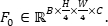Here, C = 96.
   1. Generate encoder feature maps: E₁ ∈ ℝ^{B×H/4×W/4×C}, E₂ ∈ ℝ^{B×H/8×W/8×2C}, E₃ ∈ ℝ^{B×H/16×W/16×4C}, and E₄ ∈ ℝ^{B×H/32×W/32×8C}. Use MVV Blocks containing MV4D within every encoder stage.
   2. Preserve every encoder feature for the corresponding skip connection. Pass all encoder features to MFusion Mamba for multistage feature fusion.
   3. Align encoder features to a common feature space before coarse and fine fusion within MFusion Mamba. Pass the fused representation to the decoder.
   4. Progressively upsample the decoder representation. Fuse the decoder features with E₃ at H/16 × W/16, E₂ at H/8 × W/8, and E₁ at H/4 × W/4.
   5. Upsample the final decoder feature to the original image resolution. Generate the prediction map ∈ ℝ^B×H×W×K. Here, K = 1 for binary lesion segmentation and K = 8 for Synapse multiorgan segmentation.
   6. Refer to Figure 2 for the overall network architecture and Supplementary Table 1 for the complete layer-by-layer architecture specification, including the operations, principal parameters, and output feature dimensions for each stage
   7. Encoder–decoder transition layers
      1. Downsample encoder features using patch-merging transition layers. For each transition, sample four spatially interleaved feature groups from a 2 × 2 neighborhood, concatenate them along the channel dimension, apply Layer Normalization (LayerNorm), and project the resulting 4C-dimensional feature to 2C channels using a bias-free linear layer. This operation reduces the spatial resolution by a factor of 2 while doubling the channel dimension.
      2. Upsample decoder features using patch-expanding transition layers. Apply a bias-free linear projection, rearrange the expanded features spatially to increase the resolution by a factor of 2, and apply LayerNorm after spatial expansion. Repeat this operation to progressively reconstruct the feature maps from H/32 × W/32 to H/16 × W/16, H/8 × W/8, and H/4 × W/4.
      3. Align encoder features within the MFusion Mamba module by resizing them to the target spatial resolution using bilinear interpolation (align_corners = False) and then applying a learnable linear channel projection before feature fusion.
   8. Segmentation head
      1. Upsample the final decoder feature map from H/4 × W/4 to the original image resolution (H × W) using the final patch-expanding layer. Apply linear projection, perform spatial rearrangement with an expansion factor of 4, and apply LayerNorm.
      2. Project the reconstructed feature map to K output channels using a 1 × 1 convolution after converting the tensor to channel-first format.
      3. Generate the final prediction during evaluation by applying a sigmoid activation function for binary lesion segmentation or a softmax activation followed by argmax for Synapse multiorgan segmentation. Do not apply an activation function within the segmentation head itself.

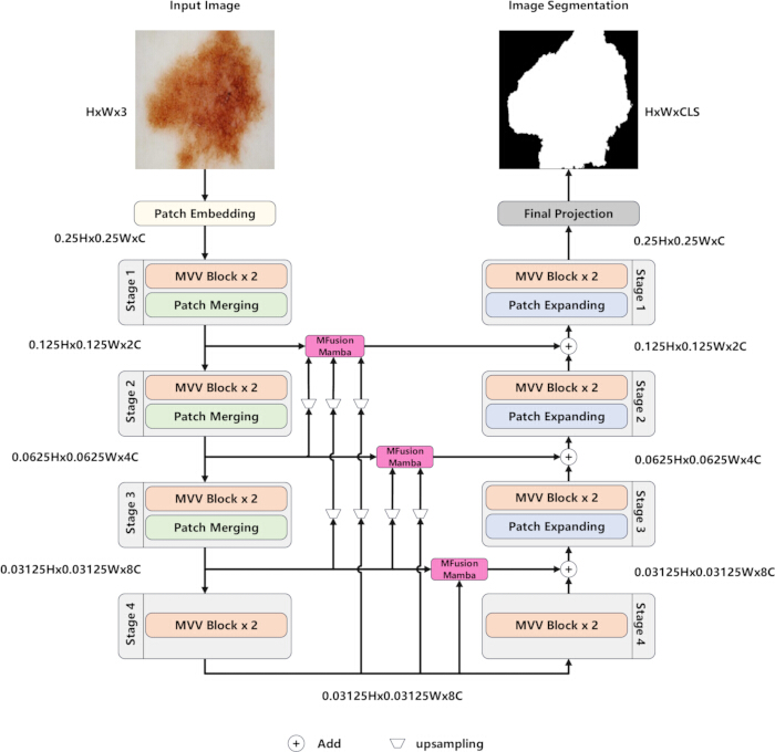
Figure 2. Overall architecture of Multi-View Mamba U-Net (MVM-UNet). Overview of the proposed Multi-View Mamba U-Net (MVM-UNet) architecture. The input image is converted into patch embeddings and processed through four encoder stages composed of Multi-View Vision (MVV) Blocks separated by patch-merging operations. Encoder features are aggregated by Multi-stage Fusion Mamba (MFusion Mamba) and propagated to the decoder through skip connections. The decoder progressively restores spatial resolution using patch-expanding operations and generates the final segmentation map through the projection layer. Please click here to view a larger version of this figure.

3. Construction of the MV4D module

1. Use the MV4D module as the basic feature extraction unit in the MVV Block. Feed the input feature patches into four scan-pair branches. Refer to Algorithm 1, Supplementary File 1 for the complete pseudocode of spatial flattening, scan-pair index construction, sequence gathering, S6/Mamba processing, inverse spatial reordering, scan-pair fusion, SFusion Mamba fusion, projection, and output reshaping.
2. Use the exact zigzag, hierarchical, spiral, and radial scan-index generation procedures implemented in models/mvmunet/core.py. For each scanning strategy, use the forward scan order and its reverse order as one bidirectional scan pair.
3. Construct the zigzag scan pair. Traverse the image features in alternating directions at the end of each row or column. Use this scan pattern to balance local and global spatial information.
4. Construct the hierarchical scan pair. Capture features at multiple spatial scales. Use this scan pattern to strengthen the extraction of both local and global representations.
5. Construct the spiral scan pair. Scan the image features from the center toward the boundary or from the boundary toward the center. Use this scan pattern to enhance the extraction of global contour information.
6. Construct the radial scan pair. Scan image features along multiple radial directions. Use this scan pattern to enhance the extraction of local boundary and edge details.
7. Merge each scan pair before feeding the merged sequence into the S6 block. Use the paired design to improve the robustness of each scanning strategy while preserving computational efficiency.
8. Feed the output sequence of each scan-pair branch into an S6 block. Obtain four feature representations corresponding to the zigzag, hierarchical, spiral, and radial scanning views.
9. Fuse the four extracted feature representations using the SFusion Mamba module. Use two parallel fusion pathways. In the first pathway, integrate the four features by element-wise addition.
10. In the second SFusion Mamba pathway, concatenate the four features. Process the concatenated representation using Conv1d and Mamba. Reduce the channel dimension using a projection layer to match the S6 block output dimension.
11. Configure the S6/Mamba block using the feature dimension C as the model dimension. Use a projection layer to map each merged scan-pair feature back to channel dimension C before fusion.
12. In SFusion Mamba, perform element-wise addition in the first pathway. Concatenate the four scan-view features in the second pathway before Conv1d, Mamba, and linear projection. Use the normalization, linear projection, depth-wise separable convolution, and activation operations surrounding MV4D as described in Step 4.
13. Add the outputs of the two fusion pathways to obtain the final output of the MV4D module.
14. Construct four complementary scan-pair branches instead of using only horizontal and vertical scanning directions. Use zigzag scanning to emphasize continuous spatial traversal, hierarchical scanning to strengthen multiscale representation, spiral scanning to capture center-to-boundary contour information, and radial scanning to enhance boundary-oriented local detail extraction.
15. Process each scan-pair branch independently. Fuse the resulting features using SFusion Mamba. Map each processed sequence back to its original spatial order before fusion.
16. Given an input feature map X ∈ ℝ^B×H×W×C, flatten it into X_seq ∈ ℝ^B×L×C, where L = H × W.
17. Reorder the flattened sequence according to the scan indices for each scan-pair branch. Process each reordered sequence using the S6 block. Restore the processed sequence to the original spatial order.
18. Fuse the four scan-view features through the additive pathway and the SFusion Mamba pathway to obtain the final MV4D output. Refer to Figure 3 for the MV4D architecture and Algorithm 1, Supplementary File 1 for the complete tensor-level implementation workflow.
19. Use the complete software implementation in models/mvmunet/core.py. This file contains the scan-index generators, PairwiseScanMamba, SequenceS6, SFusion Mamba, and the MV4D wrapper module.
20. Generate multiview scan indices
    1. Generate the scan indices by following the released implementation in models/mvmunet/core.py. For an input feature map of spatial size H × W, flatten each pixel location into a one-dimensional index using: index = r × W + c, where r and c denote the row and column coordinates, respectively.
    2. Generate the zigzag scan by traversing image diagonals with constant r + c. Collect the valid pixel indices for each diagonal and alternate the traversal direction by reversing the order of every even-numbered diagonal.
    3. Generate the hierarchical scan by recursively dividing the image into four quadrants. Visit the top-left, top-right, bottom-left, and bottom-right quadrants sequentially until the subregion height or width is no greater than 2 pixels, and then traverse the remaining pixels in row-major order.
    4. Generate the spiral scan by traversing the outer image boundary from left to right along the top row, downward along the right column, right to left along the bottom row, and upward along the left column while progressively shrinking the boundary toward the image center.
    5. Generate the radial scan by sorting each pixel according to its squared distance from the image center and then according to its polar angle calculated using the atan2 function.
    6. Generate the reverse scan for each scanning strategy by reversing the corresponding forward scan order. Combine the forward and reverse scan sequences to form one scan pair for each scanning strategy before passing the scan pairs to the MV4D module.

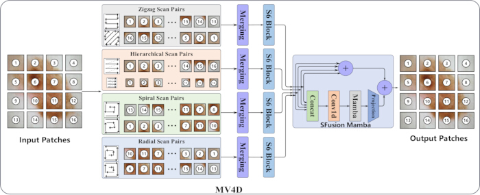
Figure 3. Architecture of the Multi-View 4-Directional (MV4D) module. Structure of the Multi-View 4-Directional (MV4D) feature extraction module. Input patches are processed through four complementary scan-pair branches, including zigzag, hierarchical, spiral, and radial scanning. Features extracted from the four branches are merged, processed using state-space blocks, and integrated by Spatial Fusion Mamba (SFusion Mamba) to generate the output feature representation. Please click here to view a larger version of this figure.

4. Construction of the MVV Block

1. Build the MVV Block using one main branch and two auxiliary branches. Use the overall structure shown in Figure 4.
2. Apply layer normalization to the input feature in the main branch. Feed the normalized feature into a linear layer. Pass the transformed feature to the depth-wise separable convolution.
3. Process the transformed feature using the depth-wise separable convolution. Apply the GELU activation function. Feed the activated feature into the MV4D module.
4. Construct the first auxiliary branch as an identity residual connection. Connect the input feature directly to the final output. Use this branch to preserve the original representation and stabilize training.
5. Construct the second auxiliary branch as a projection down-up branch. Compress the input feature using a down-projection layer. Restore the feature dimension using an up-projection layer.
6. Merge the outputs of the main branch and both auxiliary branches. Obtain the final MVV Block output. Refer to Figure 4 for the complete architecture.
7. Set the hidden dimension of the main branch equal to the input channel dimension C_s. Apply LayerNorm(C_s) before the main linear projection and use a linear layer with dimensions C_s→C_s. Use a depth-wise separable convolution consisting of a 3×3 depth-wise convolution with padding 1, groups = C_s, and no bias, followed by a 1×1 point-wise convolution without bias.
8. Apply the GELU activation function after the depth-wise separable convolution. Feed the activated feature into MV4D and apply an output linear projection with dimensions C_s→C_s. Configure the projection down-up branch using LayerNorm(C_s), a projection ratio of 4, a down-projection C_s→C_s/4, GELU activation, and an up-projection C_s/4→C_s.
9. Combine the identity branch, projection down-up branch, and drop-path-processed main branch using element-wise addition to obtain the final MVV Block output.

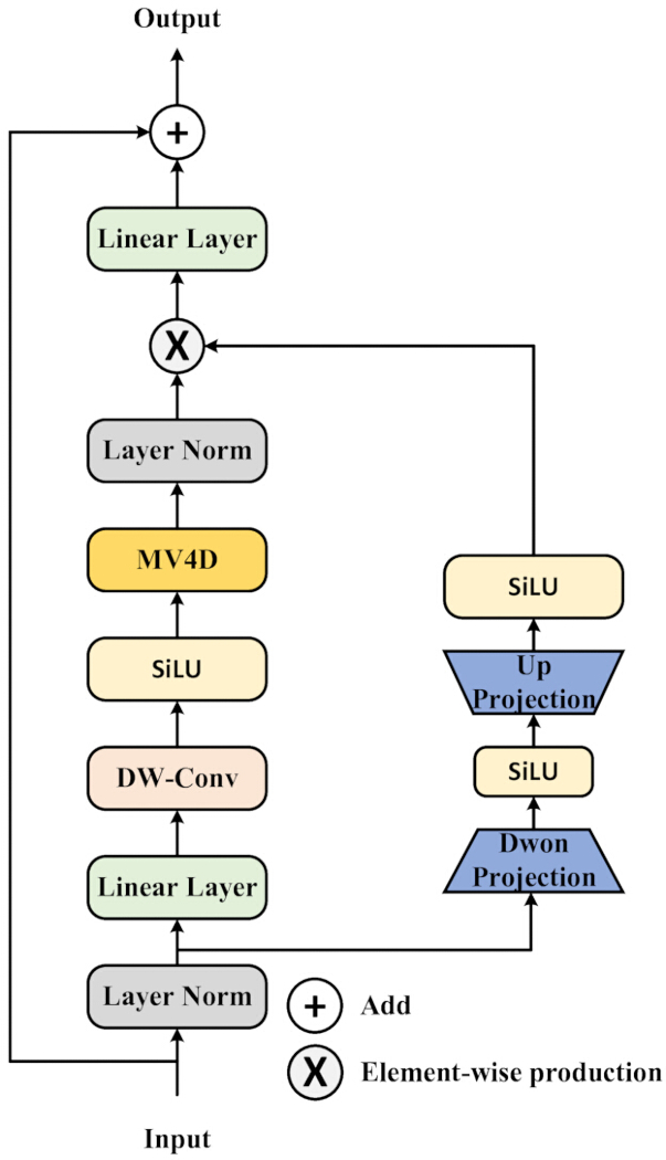
Figure 4. Architecture of the Multi-View Vision (MVV) Block. Structure of the Multi-View Vision (MVV) Block. The block consists of a main feature extraction branch containing the Multi-View 4-Directional (MV4D) module together with depthwise convolution, normalization, and linear projection layers. An auxiliary up-down projection branch provides gated feature modulation through element-wise multiplication before residual addition to generate the output feature representation. Please click here to view a larger version of this figure.

5. Construction of MFusion Mamba

1. Collect the feature maps from all encoder stages. Align the encoder features to a unified representation space by resizing or projecting them when necessary. Refer to Algorithm 2, Supplementary File 1 for the complete tensor-level implementation workflow.
2. Resize encoder features to the target spatial resolution when necessary. Project features with different channel dimensions into the same channel dimension. Align all encoder features before multistage fusion.
3. Feed the aligned encoder features into the Coarse Fusion component. Perform coarse fusion using the Hadamard product. Generate the coarse fused representation.
4. Feed the coarse fused representation into the Fine Fusion component. Construct two parallel fine-fusion pathways. Process both pathways independently.
5. Process the first Fine Fusion pathway using a linear layer. Process the second Fine Fusion pathway using up-projection, Conv1d, Mamba, and down-projection. Restore the feature dimension after down-projection.
6. Merge the outputs of the two Fine Fusion pathways using the Hadamard product. Apply the final linear layer. Obtain the MFusion Mamba output.
7. Feed the MFusion Mamba output into the decoder. Decode the fused multistage representation together with the encoder-decoder skip features. Generate the final segmentation map.
8. Align encoder features from different stages into a unified feature space before coarse fusion. Process the aligned feature representations using the coarse and fine fusion stages. Refer to Figure 5 for the MFusion Mamba architecture and Supplementary Algorithm 2 for the complete tensor-level implementation workflow.
9. Use the implementation parameters of MFusion Mamba as follows. For each encoder feature E_i, project the channel dimension from C_i to C_t. Resize projected features to the target spatial size using bilinear interpolation with align_corners=False when necessary.
10. Apply the Hadamard product to perform Coarse Fusion across the aligned encoder features. Configure the first Fine Fusion pathway using a linear layer with dimensions C_t → C_t. Configure the second Fine Fusion pathway using an up-projection C_t → 2C_t, Conv1d, a Mamba/S6 block with model dimension 2C_t, one scanning direction, state dimension 16, and a down-projection 2C_t → C_t.
11. Fuse the outputs of the Fine Fusion pathways using the Hadamard product. Apply a final linear projection with dimensions C_t to C_t. Feed the fused multistage representation into the decoder.
12. Fuse multistage encoder features using MFusion Mamba
    1. Collect the encoder features from all four encoder stages (E₁, E₂, E₃, and E₄) and use them as the input to the MFusion Mamba module. Do not select only the corresponding-stage encoder feature for decoder fusion.
    2. Align all encoder features to the spatial resolution required for the current decoder stage. Resize the encoder features to the target resolution and project them to the required channel dimension before feature fusion.
    3. Repeat the feature alignment procedure for each decoder stage. When the decoder operates at H/16 × W/16, H/8 × W/8, and H/4 × W/4, resize and project E₁, E₂, E₃, and E₄ to the corresponding target feature space.
    4. Fuse the aligned multistage encoder features using the Coarse Fusion and Fine Fusion operations of the MFusion Mamba module, and combine the fused representation with the decoder features at the corresponding scale.
    5. Perform the feature projection, resizing, and fusion operations according to the released implementation in models/mvmunet/core.py.

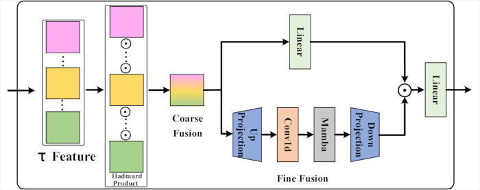
Figure 5. Architecture of the Multi-stage Fusion Mamba (MFusion Mamba) module. Structure of the Multi-stage Fusion Mamba (MFusion Mamba) module. Multi-scale encoder features are first combined by coarse fusion and subsequently refined through the Fine Fusion module consisting of linear projection, one-dimensional convolution (Conv1d), a Mamba block, and feature projection layers before generation of the fused feature representation used by the decoder. Please click here to view a larger version of this figure.

6. Model training

1. Train MVM-UNet on Ubuntu 22.04.1 with Linux kernel version 6.8.0. Use a workstation equipped with a 13th Gen Intel Core i9-13900K CPU and an NVIDIA A800 GPU. Use the same hardware configuration throughout training and evaluation.
2. Implement and train the model using PyTorch 2.0.1 with CUDA 11.8. Install all required software dependencies before training.
3. Use the AdamW optimizer with an initial learning rate of 3 × 10⁻⁵, β₁ = 0.9, β₂ = 0.999, ε = 1 × 10⁻⁸, and a weight decay of 0.01. Set the batch size to 32 unless otherwise specified.
4. Train each model for 300 epochs. Use a cosine annealing learning-rate schedule with η_min = 1 × 10⁻⁵. Set the input image size to 256 × 256 for ISIC 2017 and ISIC 2018 and to 224 × 224 for Synapse.
5. Use three independent random seeds (1, 52, and 100) for the main comparison experiments. Repeat the complete training and evaluation procedure for each seed. Report the final quantitative results as mean ± SD across the three runs.
6. Use a fixed random seed of 100 for all ablation studies unless otherwise specified. Keep the dataset partitions, preprocessing strategy, network architecture, optimizer, learning rate, batch size, and number of training epochs unchanged across all ablation experiments.
7. Use the BCE-Dice loss for binary lesion segmentation on ISIC 2017 and ISIC 2018. Set the BCE and Dice loss weights to 1.0. Use the CE-Dice loss for Synapse and set both the cross-entropy and Dice loss weights to 1.0.
8. Resize, normalize, and augment the ISIC 2017 and ISIC 2018 training images using the preprocessing procedure described in Step 1. Apply resizing, random rotation, and random flipping to Synapse training images as described in Step 1. Use identical preprocessing settings during all training runs.
9. Select model checkpoints according to the dataset-specific validation protocol. Save the checkpoint with the best validation performance for ISIC 2017 and ISIC 2018, and perform validation every 30 epochs. Train Synapse for 300 epochs without a validation set and use the final training checkpoint for testing.
10. Use the official validation set only for model selection on ISIC 2017 and ISIC 2018. Do not use the Synapse testing set for training, hyperparameter tuning, or checkpoint selection. Reserve all testing data exclusively for final evaluation.
11. Use the following training parameters for reproducibility. Set the batch size to 32 for all datasets. Use AdamW with an initial learning rate of 3 × 10⁻⁵, β₁ = 0.9, β₂ = 0.999, ε = 1 × 10⁻⁸, and a weight decay of 1 × 10⁻².
12. Configure the cosine annealing learning-rate scheduler with T_max = 50 and η_min = 1×10⁻⁵ for ISIC 2017 and ISIC 2018. Configure the scheduler with T_max = 100 and η_min = 1×10⁻⁵ for Synapse. Keep the scheduler configuration unchanged for all repeated experiments.
13. Train all models using full-precision FP32 arithmetic. Disable automatic mixed-precision training. Do not apply gradient clipping during optimization.
14. Keep the precision settings, gradient update strategy, optimizer configuration, learning-rate schedule, and random-seed protocol unchanged across all comparison experiments, ablation studies, and reproducibility runs.
15. Select the best model checkpoint
    1. Evaluate the model on the validation set after each training epoch for the ISIC 2017 and ISIC 2018 datasets.
    2. Calculate the Binary Cross-Entropy (BCE)-Dice loss for each validation batch and compute the mean validation loss across the entire validation set.
    3. Save the current model as the best checkpoint when the mean validation loss is lower than the previously recorded minimum validation loss.
    4. Record the mean Intersection over Union (mIoU), Dice Similarity Coefficient (DSC), accuracy (Acc), specificity (Spe), and sensitivity (Sen) during validation for performance monitoring only. Do not use these metrics as the checkpoint-selection criterion.

7. Model evaluation

1. Evaluate the trained model using the official testing set for each dataset. Use the testing set only for final performance assessment.
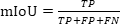
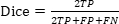
2. For ISIC 2017 and ISIC 2018, calculate the mIoU, DSC, Acc, Sen, and Spe. Use pixel-level true positives (TP), false positives (FP), true negatives (TN), and false negatives (FN) for all calculations.
3. Apply a sigmoid activation function to the model output for ISIC 2017 and ISIC 2018. Convert the probability map into a binary segmentation mask using a threshold of 0.5. Calculate the evaluation metrics using Equations 2–6:
   (2)
   (3)
   (4)
   (5)
   (6)
4. For Synapse, apply the softmax activation function to the model output. Assign each pixel or voxel to the class with the highest probability using the argmax operation. Calculate the DSC and the 95th-percentile Hausdorff distance (HD95) for each foreground organ and report the average values across all testing cases.
5. Compare MVM-UNet with representative CNN-based, Transformer-based, and state-space model (SSM)-based segmentation methods. Use identical dataset partitions, preprocessing procedures, input resolutions, and evaluation metrics for all methods.
6. Use the official training, validation, and testing partitions for ISIC 2017 and ISIC 2018. Use the standard split of 18 training cases and 12 testing cases for Synapse. Set the input resolution to for ISIC datasets and for Synapse.
7. Reproduce baseline methods using their official implementations whenever available. Report reproduced results as mean ± SD across repeated runs. Retain literature-reported values as originally published and distinguish them in the corresponding table notes.
8. Conduct ablation studies using the fixed random seed of 100 unless otherwise specified. Keep the dataset partitions, preprocessing procedure, input resolution, optimizer, learning-rate schedule, batch size, number of epochs, loss function, and evaluation metrics unchanged across all ablation experiments.
9. Evaluate the contributions of MV4D, SFusion Mamba, the Up-Down Projection branch in the MVV Block, MFusion Mamba, input image size, dropout value, and encoder-decoder layer configuration. Modify only the target component or parameter in each ablation experiment.
10. Perform the Wilcoxon signed-rank test using paired per-image results for ISIC 2017 and ISIC 2018 and paired per-case results for Synapse. Consider a p-value smaller than 0.05 to indicate statistical significance.
11. Evaluate computational efficiency using the same hardware environment and input resolution for all methods. Measure the training time per epoch, inference time per image, peak GPU memory usage during training, number of model parameters, and floating-point operations (FLOPs). Calculate FLOPs using a single forward pass.
12. Select representative qualitative examples only from the testing set after completing model evaluation. Compare the original image, ground-truth mask, and predicted mask using identical test cases across all methods. Select representative examples that include small targets, irregular boundaries, ambiguous boundaries, and representative multiorgan structures.
13. Calculate evaluation metrics and perform statistical analysis
    1. Calculate the segmentation metrics for the ISIC 2017 and ISIC 2018 datasets in Python using NumPy and sklearn.metrics.confusion_matrix. Threshold the predicted probability map at 0.5, obtain the pixel-level TP, FP, TN, and FN, and calculate the mIoU, DSC, Acc, Sen, and Spe from these values.
    2. Calculate the DSC and the HD95 for the Synapse dataset using medpy.metric.binary.dc and medpy.metric.binary.hd95, respectively. Apply softmax followed by argmax to the model output before computing the evaluation metrics.
    3. Calculate the number of FLOPs and trainable parameters using thop.profile with a single forward pass.
    4. Perform the Wilcoxon signed-rank test in Python using scipy.stats.wilcoxon. Use paired per-image metric values for the ISIC 2017 and ISIC 2018 datasets and paired per-case metric values for the Synapse dataset.

8. Loss function definition

1. Use the standard Cross-Entropy (CE) loss for multiclass segmentation and the standard BCE loss for binary segmentation. Use the standard Dice loss formulation for segmentation. Equations 7–11 define the loss functions used in this protocol.
    (7)
    (8)
    (9)
    (10)
    (11)
2. Set the BCE and Dice loss weights to 1.0 for ISIC 2017 and ISIC 2018, such that ₁ = 1.0 and ₂ = 1.0. Set the CE and Dice loss weights to 1.0 for Synapse, such φ₁ = 1.0 that and φ₂ = 1.0.
3. Implement the loss functions in utils.py. Use nn.BCELoss for the BCE term and nn.CrossEntropyLoss for the CE term. Compute the binary Dice loss by flattening each predicted mask and ground-truth mask, calculating the Dice loss for each sample, and averaging the loss across the batch. Compute the multiclass Dice loss by converting the target label map into one-hot format, applying softmax to the model output, calculating the Dice loss for each class, and averaging the loss across all classes.
4. Set the smoothing constant to 1 for the binary Dice loss and to 1×10⁻⁵ for the multiclass Dice loss. Implement the BCE-Dice loss using the BceDiceLoss class with wb = 1 and wd = 1. Implement the CE-Dice loss using the CeDiceLoss class with loss_weight = [1, 1]. Keep the smoothing constants, reduction strategy, and software implementation unchanged for all datasets, random seeds, and experiments.
5. Configure the loss reduction
   1. Instantiate nn.BCELoss() and nn.CrossEntropyLoss() without explicitly specifying the reduction argument.
   2. Use the default PyTorch loss reduction setting (reduction = "mean") for both loss functions. Do not use reduction = "sum" or an unreduced loss output.

9. Reproducibility settings and execution

1. Download the released implementation from https://github.com/LIXUEGUANG002/MVM-UNet. Use the repository together with the software packages, datasets, hardware specifications, and computational resources listed in the Table of Materials.
2. Clone the repository and enter the project directory by running git clone https://github.com/LIXUEGUANG002/MVM-UNet.git, followed by cd MVM-Unet.
3. Configure the ISIC 2017 or ISIC 2018 experiment by setting the dataset name, dataset path, input size, batch size, number of epochs, loss function, optimizer, learning-rate scheduler, and random seed in configs/config_setting.py. Run the training script from the repository root using python train.py.
4. Configure the Synapse experiment by setting the dataset name, training data path, testing volume path, list directory, input size, number of classes, batch size, number of epochs, loss function, optimizer, learning-rate scheduler, and random seed in configs/config_setting_synapse.py. Run the training script from the repository root using python train_synapse.py.
5. Perform inference-only evaluation by setting only_test_and_save_figs = True, best_ckpt_path to the trained checkpoint, and img_save_path to the output directory in the corresponding configuration file. Run python train.py for ISIC 2017 or ISIC 2018, or run python train_synapse.py for Synapse to generate prediction results and qualitative figures.
6. Use the released source code version
   1. Clone the released GitHub repository and check out commit ee891b42c2f083c4990eed72f1d4463adc5e103e on the master branch before configuring the datasets, training scripts, and evaluation settings.
   2. Use this commit to reproduce the experiments reported in this study. No tagged release version was available for the repository at the time of manuscript revision.

Results

Expected outcomes and interpretation
When this protocol is implemented correctly, the trained MVM-UNet model is expected to produce stable segmentation performance across repeated runs, with only small variations among different random seeds for most evaluation metrics. For ISIC 2017 and ISIC 2018, successful outcomes are reflected by high DSC, mIoU, Acc, Sen, and Spe values, together with predicted lesion masks that closely follow the ground-truth lesion boundaries (Figures 6 and 7). For Synapse, successful outcomes are reflected by high average DSC values and low HD95 values across the foreground organs (Figure 8). During protocol execution, quantitative metrics should be interpreted together with the corresponding qualitative segmentation results. A model that achieves a high DSC but exhibits boundary leakage, omission of small structures, or fragmented predictions should be considered only partially successful, and the preprocessing procedure, checkpoint selection, and inference settings should be verified.

Figure 6. Representative qualitative segmentation results on the ISIC 2017 dataset. Representative qualitative segmentation results obtained on the International Skin Imaging Collaboration (ISIC) 2017 skin lesion segmentation dataset. Each example shows the original dermoscopic image (Image), the corresponding ground-truth segmentation mask (GT), and the prediction generated by MVM-UNet (Pred). Representative test cases illustrate segmentation performance for lesions of varying size, morphology, and boundary complexity. Please click here to view a larger version of this figure.

Figure 7. Representative qualitative segmentation results on the ISIC 2018 dataset. Representative qualitative segmentation results obtained on the International Skin Imaging Collaboration (ISIC) 2018 skin lesion segmentation dataset. Each example shows the original dermoscopic image (Image), the corresponding ground-truth segmentation mask (GT), and the prediction generated by MVM-UNet (Pred). Representative test cases demonstrate segmentation performance across diverse lesion appearances and boundary characteristics. Please click here to view a larger version of this figure.

Figure 8. Representative qualitative segmentation results on the Synapse multiorgan computed tomography dataset. Representative qualitative multiorgan segmentation results obtained on the Synapse Multi-Atlas Labeling Beyond the Cranial Vault dataset. Each example shows the original computed tomography image (Image), the corresponding ground-truth organ annotations (GT), and the prediction generated by MVM-UNet (Pred). Representative examples illustrate agreement between predicted and reference segmentations across multiple abdominal organs. Please click here to view a larger version of this figure.

Performance on ISIC 2017
To evaluate the reproducibility of MVM-UNet, all main comparison experiments were repeated using three independent random seeds (1, 52, and 100), and the results are reported as mean ± SD. Statistical significance was evaluated using the Wilcoxon signed-rank test based on paired per-image results for ISIC 2017 and ISIC 2018 and paired per-case results for Synapse. The statistical analysis was performed using paired metric values rather than seed-level averages. For fair comparison, results reported as mean ± SD were reproduced using the official implementations under the same dataset partitions, input resolutions, and evaluation metrics whenever possible, whereas single-value results were retained from the corresponding original publications.

MVM-UNet was evaluated on the ISIC 2017 skin lesion segmentation dataset and compared with representative segmentation methods, including UNet^8,21, TransUNet²³, H-vmunet²⁸, MISSFormer³⁰, MaLUNet³¹, VM-UNet³², UNeXt-S³³, HResFormer³⁴, MedScale-Former³⁵, MCAFT³⁶, and H2Former¹² (Table 1). MVM-UNet achieved an mIoU of 80.94 ± 1.01%, a DSC of 91.32% ± 0.68%, an accuracy of 96.58% ± 0.27%, a specificity of 98.31% ± 0.23%, and a sensitivity of 91.65% ± 0.77% across three independent runs. Compared with the evaluated methods, MVM-UNet achieved the highest mIoU, DSC, and sensitivity. Representative qualitative segmentation results are shown in Figure 6, where the predicted masks closely follow the ground-truth lesion boundaries across representative test images.

Model	Ref.	mIoU (%)	DSC (%)	Acc (%)	Spe (%)	Sen (%)
UNet	8	76.98	86.99	95.65	97.43	86.82
TransUNet	23	75.32	81.23	91.45	95.77	82.63
MaLUNet	31	78.78	88.13	96.18	98.47	84.78
VM-UNet	32	80.23	89.03	96.29	97.58	89.90
UNeXt-S	33	78.26	87.80	95.95	97.74	87.04
HResFormer	34	79.89 ± 1.05	88.82 ± 0.65	96.25 ± 0.24	97.73 ± 0.22	87.72 ± 0.79
H-vmunet	28	80.34 ± 1.02	90.68 ± 0.55	96.42 ± 0.18	98.23 ± 0.32	88.97 ± 0.88
MISSFormer	30	80.16 ± 0.78	89.27 ± 0.61	94.36 ± 0.28	97.52 ± 0.38	87.71 ± 0.69
H2Former	12	80.35 ± 0.95	88.56 ± 0.72	96.61 ± 0.19	98.15 ± 0.14	88.21 ± 0.81
MedScale-Former	35	80.31 ± 0.82	89.11 ± 0.59	95.68 ± 0.33	98.24 ± 0.21	89.96 ± 0.92
MCAFT	36	80.59 ± 0.93	89.27 ± 0.63	96.42 ± 0.20	97.95 ± 0.17	90.05 ± 0.84
MVM-UNet (Ours)	—	80.94 ± 1.01	91.32 ± 0.68	96.58 ± 0.27	98.31 ± 0.23	91.65 ± 0.77

Table 1: Performance comparison on the ISIC 2017 skin lesion segmentation dataset. Comparison of MVM-UNet with representative convolutional neural network (CNN)-, Transformer-, and state-space model (SSM)-based segmentation methods using mean Intersection over Union (mIoU), Dice Similarity Coefficient (DSC), accuracy (Acc.), specificity (Spe.), and sensitivity (Sen.). Results for MVM-UNet are reported as mean ± standard deviation from three independent random-seed experiments. Results reported as single values were reproduced from the corresponding original publications.

The qualitative examples further demonstrate that MVM-UNet accurately segmented both small lesions and larger lesions with irregular boundaries. In these representative examples, the predicted masks closely matched the corresponding ground-truth annotations and preserved lesion boundaries with minimal leakage or fragmentation.

To further evaluate whether the observed improvements were statistically significant, Wilcoxon signed-rank tests were performed using paired per-image segmentation results. For the mIoU metric, MVM-UNet showed a statistically significant improvement over MCAFT, with a p-value of 0.0114. For the DSC metric, MVM-UNet also significantly outperformed H-vmunet, with a p-value of 0.0031. These results support that the observed improvements on ISIC 2017 were unlikely to be attributable to random variation.

Overall, MVM-UNet achieved the highest performance among the compared methods for mIoU, DSC, and sensitivity on the ISIC 2017 dataset (Table 1). The qualitative segmentation examples shown in Figure 6 are consistent with these quantitative findings.

Performance on ISIC 2018
MVM-UNet was further evaluated on the ISIC 2018 skin lesion segmentation dataset and compared with representative segmentation methods, including UNet^8,21, UNet++⁹, UTNetV2³⁷, SANet³⁸, MaLUNet³¹, VM-UNet³², H-vmunet²⁸, MISSFormer³⁰, H2Former¹², HResFormer³⁴, MedScale-Former³⁵, and MCAFT³⁶ (Table 2). MVM-UNet achieved an mIoU of 82.47% ± 1.28%, a DSC of 90.65% ± 0.94%, an accuracy of 96.02% ± 0.36%, a specificity of 97.06% ± 0.31%, and a sensitivity of 91.80% ± 0.82% across three independent runs. These results demonstrate that the performance of MVM-UNet remained consistent across different random seeds. Representative qualitative segmentation results are shown in Figure 7.

Model	Ref.	mIoU (%)	DSC (%)	Acc (%)	Spe (%)	Sen (%)
UNet	8	77.86	87.55	94.05	96.69	85.86
UNet++	9	78.31	87.83	94.02	95.75	88.65
UTNetV2	37	78.97	88.25	94.32	96.48	87.60
SANet	38	79.52	88.59	94.39	95.97	89.46
MaLUNet	31	80.25	89.04	94.62	96.19	89.74
VM-UNet	32	81.35	89.71	94.91	96.13	91.12
H-vmunet	28	81.93 ± 1.45	90.46 ± 0.62	95.19 ± 0.30	96.82 ± 0.21	88.37 ± 1.13
MISSFormer	30	80.27 ± 1.21	89.91 ± 0.46	94.76 ± 0.27	97.22 ± 0.15	90.84 ± 1.07
H2Former	12	80.40 ± 0.83	90.26 ± 0.73	94.89 ± 0.38	96.98 ± 0.25	91.57 ± 0.54
HResFormer	34	81.12 ± 1.18	88.86 ± 0.84	94.96 ± 0.33	96.43 ± 0.22	91.86 ± 1.01
MedScale-Former	35	80.97 ± 0.74	90.47 ± 0.68	95.02 ± 0.41	95.89 ± 0.26	90.65 ± 0.92
MCAFT	36	81.46 ± 1.03	89.06 ± 0.76	95.23 ± 0.29	96.72 ± 0.17	91.82 ± 0.57
MVM-UNet (Ours)	—	82.47 ± 1.28	90.65 ± 0.94	96.02 ± 0.36	97.06 ± 0.31	91.80 ± 0.82

Table 2: Performance comparison on the ISIC 2018 skin lesion segmentation dataset. Comparison of MVM-UNet with representative CNN-, Transformer-, and SSM-based segmentation methods using mean Intersection over Union (mIoU), Dice Similarity Coefficient (DSC), accuracy (Acc.), specificity (Spe.), and sensitivity (Sen.). Results for MVM-UNet are reported as mean ± standard deviation from three independent random-seed experiments. Results reported as single values were reproduced from the corresponding original publications.

Compared with H-vmunet, MVM-UNet improved the mIoU by 0.54%. Compared with MedScale-Former, MVM-UNet improved the DSC by 0.18%. MVM-UNet also achieved the highest accuracy among the compared methods. The representative qualitative examples shown in Figure 7 demonstrate accurate segmentation of representative skin lesions, including small lesion regions and lesions with irregular boundaries.

For ISIC 2018, statistical significance was evaluated using the Wilcoxon signed-rank test based on paired per-image segmentation results. For the mIoU metric, MVM-UNet achieved a statistically significant improvement over MCAFT, with a p-value of < 0.001. These results support that the observed performance improvement on ISIC 2018 was unlikely to be attributable to random variation.

Overall, MVM-UNet achieved the highest mIoU, DSC, and accuracy among the compared methods on the ISIC 2018 dataset (Table 2). The qualitative examples shown in Figure 7 are consistent with these quantitative improvements.

Performance on Synapse
The proposed method was also evaluated on the Synapse multiorgan segmentation dataset and compared with representative methods, including UNet^8,21, Attention U-Net³⁹, TransUNet²³, TransNorm⁴⁰, Swin U-Net²⁵, TransDeepLab⁴¹, MEW-UNet⁴², MISSFormer³⁰, H2Former¹², HResFormer³⁴, MedScale-Former³⁵, and MCAFT³⁶ (Table 3). The Synapse dataset included eight abdominal organs: the aorta, gallbladder, spleen, left kidney, right kidney, liver, pancreas, and stomach. Following the standard experimental protocol, 18 cases (2,212 axial slices) were used for training and 12 cases (1,567 axial slices) were used for testing. No separate validation set was introduced. The testing cases were used exclusively for final evaluation and were not used for model training, hyperparameter tuning, or model selection. Representative qualitative multiorgan segmentation results are shown in Figure 8, and the quantitative comparison is summarized in Table 3.

Model	Ref.	DSC	HD95	Aor.	Gal.	Kid. (L)	Kid. (R)	Liv.	Pan.	Spl.	Sto.
UNet	8	76.85	39.78	89.07	69.72	77.77	68.69	93.43	54.01	86.66	75.59
Att-UNet	39	77.77	36.02	89.54	68.88	77.98	71.11	93.57	58.04	87.31	75.74
TransUNet	23	77.48	31.69	87.23	63.13	81.87	77.02	94.08	55.84	85.06	75.62
TransNorm	40	78.4	30.25	86.23	65.18	82.18	78.63	94.22	55.32	89.53	76.02
Swin U-Net	25	79.13	21.55	85.47	66.53	83.28	79.61	94.29	56.58	90.62	76.59
TransDeepLab	41	80.16	21.25	86.04	69.16	84.08	79.88	93.53	61.15	89.01	78.36
MEW-UNet	42	78.92	21.68	86.68	65.32	82.87	80.02	93.63	58.38	90.16	74.27
MISSFormer	30	80.92 ± 4.23	20.09 ± 1.89	86.43 ± 0.98	69.81 ± 4.56	84.29 ± 2.11	81.03 ± 3.34	93.85 ± 0.89	61.11 ± 4.67	90.05 ± 3.78	80.62 ± 1.02
H2Former	12	81.05 ± 2.56	20.13 ± 7.23	86.61 ± 3.21	69.32 ± 1.23	85.12 ± 4.78	82.01 ± 2.89	94.09 ± 2.45	61.16 ± 0.76	89.97 ± 4.12	80.94 ± 3.56
HResFormer	34	80.65 ± 4.02	17.48 ± 6.89	89.16 ± 2.78	66.94 ± 0.78	84.61 ± 4.34	82.15 ± 2.56	93.11 ± 1.34	59.92 ± 4.12	91.08 ± 3.45	80.75 ± 2.01
MedScale-Former	35	80.78 ± 1.34	20.02 ± 3.78	88.79 ± 4.02	69.82 ± 2.56	85.13 ± 0.87	81.63 ± 4.78	94.10 ± 2.78	60.72 ± 1.89	90.14 ± 1.56	80.93 ± 4.56
MCAFT	36	81.03 ± 3.45	19.98 ± 5.12	89.76 ± 0.76	68.96 ± 3.89	84.54 ± 2.56	81.98 ± 3.12	94.32 ± 4.01	60.85 ± 3.67	89.06 ± 4.89	80.91 ± 1.78
MVM-UNet (Ours)	—	81.26 ± 1.89	18.72 ± 2.16	88.53 ± 3.22	69.84 ± 4.23	85.37 ± 2.69	82.67 ± 1.67	94.41 ± 3.56	61.02 ± 2.78	90.19 ± 0.67	81.48 ± 3.12

Table 3: Performance comparison on the Synapse multi-organ segmentation dataset. Comparison of MVM-UNet with representative CNN-, Transformer-, and SSM-based segmentation methods using the Dice Similarity Coefficient (DSC), 95th-percentile Hausdorff distance (HD95), and organ-specific Dice scores for the aorta (Aor.), gallbladder (Gal.), left kidney (Kid. (L)), right kidney (Kid. (R)), liver (Liv.), pancreas (Pan.), spleen (Spl.), and stomach (Sto.). Results for MVM-UNet are reported as mean ± standard deviation from three independent random-seed experiments. Results reported as single values were reproduced from the corresponding original publications.

MVM-UNet achieved a mean DSC of 81.26% ± 1.89% and a mean HD95 of 18.72 ± 2.16 across three independent runs. The results demonstrate stable segmentation performance on the Synapse dataset. Among the evaluated methods, MVM-UNet achieved the highest average DSC and the second-lowest average HD95.

For Synapse, statistical significance was evaluated using the Wilcoxon signed-rank test based on paired per-case DSC values. MVM-UNet showed a statistically significant improvement over H2Former, with a p-value of 0.026, indicating that the observed improvement in segmentation performance was statistically significant.

Representative successful and suboptimal outcomes
Representative successful qualitative results are shown in Figures 6–8. Successful outcomes are characterized by predicted segmentation masks that closely correspond to the ground-truth annotations and accurately delineate the primary lesion or organ boundaries. Representative suboptimal outcomes may occur for very small targets, low-contrast boundaries, irregular lesion shapes, organs with weak intensity contrast, or anatomically ambiguous boundaries, and typically appear as under-segmentation, over-segmentation, boundary leakage, or discontinuous mask fragments. When such outcomes are observed, users should verify that image resizing, normalization, mask interpolation, model checkpoint selection, inference thresholding (for ISIC datasets) or argmax prediction (for Synapse), and metric calculation procedures are consistent with those described in the Protocol.

Ablation study of the MV4D module
The contribution of the MV4D module was evaluated by progressively adding the zigzag, hierarchical, spiral, and radial scan pairs, followed by the SFusion Mamba module (Table 4; Figure 9). When only the zigzag scan pair was used, segmentation performance was limited. Adding the hierarchical scan pair substantially improved performance, indicating the benefit of incorporating multiscale information. The subsequent addition of the spiral and radial scan pairs further improved segmentation performance by enhancing contour and boundary representation. Incorporation of the SFusion Mamba module resulted in the highest performance among the evaluated configurations.

Model	Zigzag scan pair	Hierarchical scan pair	Spiral scan pair	Radial scan pair	SFusion Mamba	ISIC 2017 mIoU (%)	ISIC 2017 DSC (%)	ISIC 2018 mIoU (%)	ISIC 2018 DSC (%)
MVM-UNet	✓					56.75	72.46	58.03	73.45
MVM-UNet	✓	✓				72.38	84.01	73.45	84.7
MVM-UNet	✓	✓	✓			75.69	86.20	76.94	86.94
MVM-UNet	✓	✓	✓	✓		76.41	86.61	78.28	87.82
MVM-UNet	✓	✓	✓	✓	✓	80.94	91.32	82.47	90.65

Table 4: Ablation study of the Multi-View 4-Directional (MV4D) module. Performance obtained by progressively incorporating the hierarchical, spiral, and radial scan pairs and the Spatial Fusion Mamba (SFusion Mamba) module into the baseline zigzag scan-pair architecture. Performance is reported using mean Intersection over Union (mIoU) and Dice Similarity Coefficient (DSC) on the ISIC 2017 and ISIC 2018 datasets.

Figure 9. Ablation study of the Multi-View 4-Directional (MV4D) module. (A) Change in mean Intersection over Union (mIoU) following sequential incorporation of the hierarchical scan pair, spiral scan pair, radial scan pair, and Spatial Fusion Mamba (SFusion Mamba) into the baseline architecture. (B) Change in the Dice Similarity Coefficient (DSC) following sequential incorporation of the hierarchical scan pair, spiral scan pair, radial scan pair, and Spatial Fusion Mamba (SFusion Mamba) into the baseline architecture. (C) Change in mIoU following sequential incorporation of the hierarchical scan pair, spiral scan pair, radial scan pair, and Spatial Fusion Mamba (SFusion Mamba) into the baseline architecture under the second experimental setting. (D) Change in the DSC following sequential incorporation of the hierarchical scan pair, spiral scan pair, radial scan pair, and Spatial Fusion Mamba (SFusion Mamba) into the baseline architecture under the second experimental setting. Please click here to view a larger version of this figure.

On the ISIC 2017 dataset, the complete MV4D module achieved an mIoU of 80.94% and a DSC of 91.32%. The corresponding performance trends for mIoU and DSC are shown in Figure 9A and Figure 9B, respectively. On the ISIC 2018 dataset, the complete MV4D module achieved an mIoU of 82.47% and a DSC of 90.65%. The corresponding performance trends are shown in Figure 9C and Figure 9D, respectively.

Unless otherwise specified, all ablation experiments were conducted using a fixed random seed of 100, whereas the main comparison results were reported as mean ± SD over three independent random seeds (1, 52, and 100). Consequently, the ablation results are intended to compare the relative contributions of individual components under a controlled single-seed setting rather than to reproduce the final multiseed performance reported in the main comparison experiments.

Overall, progressively incorporating the additional scan pairs and the SFusion Mamba module consistently improved segmentation performance, with the complete MV4D configuration achieving the highest performance on both datasets.

Ablation study of the Multi-View Vision (MVV) Block
The MVV Block was evaluated by comparing the baseline architecture with a version incorporating the Up-Down Projection branch (Table 5). On the ISIC 2017 dataset, inclusion of the Up-Down Projection branch increased the mIoU from 78.83% to 80.96% and the DSC from 88.15% to 91.02%. On the ISIC 2018 dataset, the mIoU increased from 80.32% to 82.46%, while the DSC increased from 89.15% to 90.57%.

Model	Baseline MVV Block	Up-Down Projection	ISIC 2017 mIoU (%)	ISIC 2017 DSC (%)	ISIC 2018 mIoU (%)	ISIC 2018 DSC (%)
MVM-UNet	✓		78.83	88.15	80.32	89.15
MVM-UNet	✓	✓	80.96	91.02	82.46	90.57

Table 5: Ablation study of the Multi-View Vision (MVV) Block. Performance comparison of the baseline Multi-View Vision (MVV) Block with and without the Up-Down Projection branch. Performance is reported using mean Intersection over Union (mIoU) and Dice Similarity Coefficient (DSC) on the ISIC 2017 and ISIC 2018 datasets.

The MVV Block ablation experiments were conducted using the fixed random seed of 100. Consequently, the performance of the configuration containing the Up-Down Projection branch reflects the controlled single-seed ablation setting and may differ slightly from the three-seed mean performance reported for the complete MVM-UNet model in the main comparison experiments.

Overall, incorporation of the Up-Down Projection branch consistently improved segmentation performance on both datasets, with increases observed for both mIoU and DSC.

Ablation study of the Multi-stage Fusion Mamba (MFusion Mamba) module
The MFusion Mamba module was evaluated by comparing different coarse fusion strategies together with the Fine Fusion component (Table 6; Figure 10). Without MFusion Mamba, MVM-UNet achieved an mIoU of 75.47% and a DSC of 86.01% on the ISIC 2017 dataset, and an mIoU of 77.49% and a DSC of 87.29% on the ISIC 2018 dataset. Among the evaluated coarse fusion strategies, the Hadamard product achieved the largest improvement. Incorporation of the Fine Fusion component further increased segmentation performance. The complete MFusion Mamba configuration achieved an mIoU of 80.95% and a DSC of 91.18% on ISIC 2017, and an mIoU of 82.51% and a DSC of 90.58% on ISIC 2018.

Model	Coarse FusionElement-wise Maximum	Coarse FusionElement-wise Addition	Coarse FusionHadamard Product	Fine Fusion Module	ISIC 2017 mIoU (%)	ISIC 2017 DSC (%)	ISIC 2018 mIoU (%)	ISIC 2018 DSC (%)
MVM-UNet					75.47	86.01	77.49	87.29
MVM-UNet	✓				76.21	86.47	78.35	87.82
MVM-UNet		✓			76.83	86.86	79.11	88.30
MVM-UNet			✓		78.26	87.83	80.06	88.96
MVM-UNet			✓	✓	80.95	91.18	82.51	90.58

Table 6: Ablation study of the Multi-stage Fusion Mamba (MFusion Mamba) module. Performance comparison of different Coarse Fusion strategies, including maximum fusion (Max), element-wise addition (⊕), and Hadamard product (⊙), together with the complete Fine Fusion module. Performance is reported using mean Intersection over Union (mIoU) and Dice Similarity Coefficient (DSC) on the ISIC 2017 and ISIC 2018 datasets.

Figure 10. Ablation study of the Multi-stage Fusion Mamba (MFusion Mamba) module. (A) Change in mean Intersection over Union (mIoU) obtained using different coarse fusion strategies (maximum, element-wise addition, and Hadamard product) and the complete Fine Fusion module. (B) Change in the Dice Similarity Coefficient (DSC) obtained using different coarse fusion strategies (maximum, element-wise addition, and Hadamard product) and the complete Fine Fusion module. (C) Change in mIoU obtained using different coarse fusion strategies (maximum, element-wise addition, and Hadamard product) and the complete Fine Fusion module under the second experimental setting. (D) Change in the DSC obtained using different coarse fusion strategies (maximum, element-wise addition, and Hadamard product) and the complete Fine Fusion module under the second experimental setting. Please click here to view a larger version of this figure.

On the ISIC 2017 dataset, the complete MFusion Mamba configuration achieved an mIoU of 80.95% and a DSC of 91.18%. The corresponding performance trends for mIoU and DSC are shown in Figure 10A and Figure 10B, respectively. On the ISIC 2018 dataset, the complete MFusion Mamba configuration achieved an mIoU of 82.51% and a DSC of 90.58%. The corresponding performance trends are shown in Figure 10C and Figure 10D, respectively. The MFusion Mamba ablation experiments were conducted using the fixed random seed of 100. Consequently, the complete MFusion Mamba configuration represents the controlled single-seed ablation result and may differ slightly from the three-seed mean performance reported for the complete MVM-UNet model in the main comparison experiments.

Overall, progressively incorporating the Hadamard-product coarse fusion strategy and the Fine Fusion component consistently improved segmentation performance, with the complete MFusion Mamba configuration achieving the highest performance on both datasets.

Summary of ablation studies
Across the ablation experiments, progressively incorporating the hierarchical, spiral, and radial scan-pair branches, together with the SFusion Mamba module, consistently improved segmentation performance (Table 4; Figure 9). Similarly, inclusion of the Up-Down Projection branch in the MVV Block improved both mIoU and DSC on the ISIC 2017 and ISIC 2018 datasets (Table 5). The complete MFusion Mamba configuration also achieved the highest performance among the evaluated multistage feature fusion strategies (Table 6; Figure 10).

Ablation study of hyperparameters
The effects of input size and dropout value were evaluated on the ISIC 2017 and ISIC 2018 datasets (Table 7). Three input resolutions (256 × 256, 384 × 384, and 512 × 512) were compared. Under the evaluated settings, the 256 × 256 input resolution achieved the highest segmentation performance on both datasets.

Model	Input size 256 × 256	Input size 384 × 384	Input size 512 × 512	Dropout 0.0	Dropout 0.1	Dropout 0.2	Dropout 0.3	ISIC 2017 mIoU (%)	ISIC 2017 DSC (%)	ISIC 2018 mIoU (%)	ISIC 2018 DSC (%)
MVM-UNet		✓				✓		80.02	88.91	81.76	89.92
MVM-UNet			✓			✓		79.96	88.87	80.97	89.47
MVM-UNet	✓			✓				77.48	87.28	78.76	88.11
MVM-UNet	✓				✓			79.36	88.53	81.13	89.62
MVM-UNet	✓					✓		80.94	90.15	82.49	90.50
MVM-UNet	✓						✓	79.71	88.71	80.46	89.18

Table 7: Ablation study of input image size and dropout value. Performance comparison of MVM-UNet using different input image sizes and dropout values. Segmentation performance is reported using mean Intersection over Union (mIoU) and Dice Similarity Coefficient (DSC) on the ISIC 2017 and ISIC 2018 datasets.

Different dropout values were also evaluated. Among the tested configurations, a dropout value of 0.2 achieved the highest segmentation performance on both datasets and was therefore used in the main experiments.

Ablation study of encoder-decoder layer configuration
Different encoder-decoder layer configurations were evaluated to examine the effect of network depth on segmentation performance and computational cost (Table 8). Among the evaluated configurations, the symmetric {2, 2, 2, 2}-{2, 2, 2, 2} architecture achieved the highest overall segmentation performance while maintaining relatively low model complexity. Increasing the network depth to {2, 2, 9, 2}-{2, 9, 2, 2} produced comparable segmentation performance but increased both the number of parameters and the computational cost.

Model	Encoder-decoder layer configuration	Parameters (M)	FLOPs (G)	ISIC 2017 mIoU (%)	ISIC 2017 DSC (%)	ISIC 2018 mIoU (%)	ISIC 2018 DSC (%)
MVM-UNet	{2,2,2,1}-{2,2,2,2}	28.22	4.12	80.02	88.91	81.16	89.64
MVM-UNet	{2,2,2,2}-{2,2,2,2}	28.36	4.39	80.95	90.17	82.5	90.41
MVM-UNet	{2,2,2,3}-{2,3,2,2}	30.14	4.88	79.83	88.8	81.56	89.85
MVM-UNet	{2,4,2,2}-{2,2,4,2}	33.46	5.32	79.65	88.7	81.45	89.79
MVM-UNet	{2,2,9,2}-{2,9,2,2}	45.63	7.78	80.96	90.09	82.48	90.43

Table 8: Ablation study of encoder-decoder layer configurations. Performance comparison of different encoder-decoder layer configurations. The table reports the number of model parameters (Parameters), floating-point operations (FLOPs), mean Intersection over Union (mIoU), and Dice Similarity Coefficient (DSC) on the ISIC 2017 and ISIC 2018 datasets.

Computational cost comparison
The computational efficiency of the final MVM-UNet model was compared with representative baseline methods, including HResFormer, H-vmunet, MISSFormer, H2Former, MedScale-Former, and MCAFT, under the same hardware environment and input resolution (Table 9). The evaluated metrics included training time per epoch, inference time per image, peak GPU memory usage during training, number of trainable parameters (Params), and FLOPs. Training time was measured as the time required to complete one training epoch, inference time was measured as the average processing time per test image, and FLOPs were calculated for a single forward pass.

Method	Ref.	Training time (s/epoch)	Inference time (ms/image)	Peak GPU memory (GB)	Parameters (M)	FLOPs (G)
HResFormer	34	520	213.08	19.2	117.00	131.70
H-vmunet	28	88	27.00	5.0	10.74	8.97
MISSFormer	30	355	92.86	12.6	42.33	109.45
H2Former	12	130	29.02	8.8	33.71	33.56
MedScale-Former	35	80	23.50	5.9	4.96	3.79
MCAFT	36	145	34.00	8.7	30.00	12.00
MVM-UNet (Ours)	—	104	26.80	7.9	28.36	4.39

Table 9: Computational cost comparison of MVM-UNet and representative baseline methods. Comparison of computational efficiency under the same hardware environment and input resolution. Reported metrics include training time per epoch, inference time per image, peak graphics processing unit (GPU) memory usage during training, number of model parameters (Parameters), and floating-point operations (FLOPs). Methods with available implementations were evaluated using the same experimental environment whenever possible.

As summarized in Table 9, MVM-UNet required 104 s per training epoch, 26.8 ms per image for inference, 7.9 GB of peak GPU memory, 28.36 million trainable parameters, and 4.39 GFLOPs. Compared with HResFormer, MISSFormer, H2Former, and MCAFT, MVM-UNet required lower training time, lower inference time, lower peak GPU memory usage, and fewer FLOPs. Compared with the lightweight H-vmunet and MedScale-Former models, MVM-UNet required greater training time and memory usage but maintained comparable inference speed while retaining relatively low computational complexity.

Data and Code Availability
The ISIC 2017 and ISIC 2018 datasets are publicly available from the International Skin Imaging Collaboration (ISIC) archive, and the Synapse dataset is publicly available from the Synapse repository. Dataset acquisition details are provided in the Ethics statement. Briefly, the ISIC 2017 dataset was obtained from the official ISIC 2017 Challenge data repository (https://challenge.isic-archive.com/data/#2017), the ISIC 2018 dataset was obtained from the official ISIC 2018 Challenge Task 1 data repository (https://challenge.isic-archive.com/data/#2018), and the Synapse dataset was obtained from the Synapse repository under accession identifier syn3193805 (https://www.synapse.org/Synapse:syn3193805). The corresponding download dates are reported in the Ethics statement. An initial public version of the MVM-UNet source code is available at https://github.com/LIXUEGUANG002/MVM-UNet. The repository includes the model implementation, major network modules, configuration files, dataset organization instructions, training scripts, and evaluation scripts. The complete reproducibility package, including finalized configuration files, complete experiment scripts, additional documentation, and trained model checkpoints, will be made publicly available upon publication.

Supplementary Table 1. Layer-by-layer architecture of the Multi-view Vision Mamba UNet (MVM-UNet). The table summarizes the sequential network architecture of MVM-UNet, including the input layer, patch embedding, encoder stages, Multi-View Vision (MVV) Blocks, patch-merging operations, Multi-stage Fusion Mamba (MFusion Mamba), decoder stages, final upsampling, and segmentation head. For each stage, the corresponding operation, principal parameters, and output feature size are listed. E1–E4 denote the encoder-stage feature maps used for multistage feature fusion. B, H, and W denote the batch size, image height, and image width, respectively, and K denotes the number of output classes (K = 1 for binary skin lesion segmentation and K = 9 for Synapse multiclass segmentation, comprising one background class and eight foreground organ classes). MFusion Mamba generates fused multistage encoder features that are integrated with the corresponding decoder features during decoder reconstruction. Please click here to download this file.

Supplementary File 1. Pseudocode of the Multi-View Four-Directional (MV4D) module and Multi-stage Fusion Mamba (MFusion Mamba). The supplementary file presents the algorithmic workflow of the two principal modules used in MVM-UNet. Algorithm 1 describes the complete processing pipeline of the Multi-View Four-Directional (MV4D) module, including feature flattening, construction of four scan-pair sequences (zigzag, hierarchical, spiral, and radial), selective state-space (S6) processing, Scan-view Fusion Mamba (SFusion Mamba), and reconstruction of the output feature map. Algorithm 2 describes the Multi-stage Fusion Mamba (MFusion Mamba) module, including multistage encoder feature alignment, coarse fusion, fine fusion, decoder integration, and generation of the fused decoder input feature. Variables and tensor dimensions are defined within the algorithms. Please click here to download this file.

Supplementary Coding File 1. Source code package for MVM-UNet (MVM-UNet-master). The supplementary ZIP archive contains the complete source-code implementation of MVM-UNet used in this study. The package includes the network architecture, Multi-View Four-Directional (MV4D) and Multi-stage Fusion Mamba (MFusion Mamba) modules, configuration files, training and evaluation scripts for the ISIC 2017, ISIC 2018, and Synapse datasets, utility functions, and project documentation required to reproduce the experiments described in this protocol. The package also includes the README file with installation instructions, software dependencies, dataset organization, and training and inference workflows. Please click here to download this file.

Discussion

This protocol describes MVM-UNet, a Mamba-based medical image segmentation framework. The method was designed to address two limitations of existing segmentation models. First, conventional CNN-based methods have limited ability to model long-range dependencies and hierarchical contextual information in complex medical images⁴³. Second, Transformer-based methods can model global context but usually require higher computational cost^23,25. MVM-UNet uses the Mamba architecture^{13,14,15,16,17,18,19,20} to achieve efficient long-range modeling and introduces multiview scanning and multistage feature fusion to improve segmentation accuracy. From the perspective of protocol execution and reproducibility, several steps are critical for obtaining results comparable to those reported in this study. First, the dataset split, image resizing, mask interpolation, normalization strategy, and channel conversion should be kept consistent with the protocol because differences in preprocessing can directly change the input distribution and mask boundaries. In particular, segmentation masks should be resized using nearest-neighbor interpolation to avoid introducing non-integer label values⁴⁴. Second, the training configuration, including the input resolution, batch size, optimizer settings, learning-rate schedule, random seed, loss weighting coefficients, checkpoint selection rule, and inference threshold or argmax operation, should be checked before comparing results. If reproduced results are clearly lower than the reported values, users should first verify the dataset path, annotation format, foreground-background label convention, checkpoint loading, validation or testing split, and metric calculation procedure. Boundary leakage, fragmented masks, or missing small structures usually indicate potential inconsistencies in preprocessing, mask interpolation, checkpoint selection, or inference post-processing.

The main contribution of MVM-UNet is the MV4D module. Unlike simple two-dimensional scanning strategies adopted in previous state-space-model-based architectures^{14,15,16,17,18,19,20}, MV4D uses zigzag, hierarchical, spiral, and radial scan pairs to capture complementary visual information. Zigzag scan pairs help balance local and global spatial information, hierarchical scan pairs enhance multiscale feature extraction, spiral scan pairs strengthen global contour representation, and radial scan pairs improve local edge and boundary feature extraction. SFusion Mamba then integrates these complementary scanning modalities. The representative results and ablation experiments (Tables 4 and 5; Figure 9) demonstrate that both the diversity of scan patterns and the fusion mechanism contribute to improved segmentation performance. Another important component is MFusion Mamba, which serves as a feature fusion module between the encoder and decoder. Conventional U-shaped architectures, including U-Net^8,21, V-Net⁴⁴, and many subsequent variants^9,23,25, primarily transfer information through stage-wise skip connections. This strategy may not fully exploit complementary multistage encoder representations. MFusion Mamba addresses this limitation by combining encoder features through Coarse Fusion and Fine Fusion before decoding. The representative results (Table 6; Figure 10) show that MFusion Mamba consistently improves segmentation performance, indicating that explicit multistage feature fusion is beneficial for medical image segmentation.

The methodological contribution of MVM-UNet should be understood as an architecture-level redesign rather than the invention of every individual operation from scratch. U-shaped encoder-decoder architectures, residual connections, projection layers, and Mamba/state-space model (SSM) blocks have been extensively investigated in previous studies^{8,13,14,15,16,17,18,19,20,21,23,24,25,29,44}. However, directly combining these components does not necessarily address the specific challenges of medical image segmentation. The novelty of MVM-UNet lies in the coordinated design of three aspects. First, the MV4D module replaces a single or limited scanning pattern with four complementary scan-pair branches, enabling the model to capture spatial continuity, multiscale structure, global contour information, and local boundary details. Second, SFusion Mamba and the MVV Block fuse and enhance scan-specific features before they are passed to the next network stage. Third, MFusion Mamba explicitly aggregates multistage encoder features before decoding, complementing conventional skip connections^8,21,44 and improving the use of hierarchical information. The ablation results (Tables 4–6; Figures 9 and 10) further support this design rationale, showing that multiview scanning, scan-specific fusion, the Up-Down Projection branch, and multistage feature fusion each contribute to improved segmentation performance. Therefore, the contribution of MVM-UNet lies in a task-specific and experimentally validated integration of Mamba-based spatial modeling and encoder-decoder feature fusion for medical image segmentation.

Despite its strong performance, MVM-UNet has several limitations. First, segmentation performance did not consistently improve with larger input image sizes, suggesting that the current architecture may not fully exploit high-resolution image information. Second, the model was not extensively evaluated under high-noise or low-contrast imaging conditions, which are frequently encountered in clinical practice and may affect segmentation robustness. Third, although the model achieved strong performance on three publicly available datasets, further validation on larger and more diverse medical imaging datasets is warranted. The protocol can be adapted to other medical image segmentation tasks, but several modifications should be implemented carefully. For a new binary segmentation task, users should modify the dataset loader, normalization parameters, input resolution, and foreground threshold while maintaining the binary BCE-Dice loss and evaluation procedure. For a new multiclass segmentation task, users should update the number of output classes, class-index mapping, one-hot label conversion, CE-Dice loss configuration, and class-wise evaluation metrics⁴⁴. For grayscale datasets, the input-channel configuration should be matched to the model architecture by either using a single-channel input projection or repeating the grayscale image to create a three-channel input, depending on the implementation. The method may perform suboptimally when target structures are extremely small, boundaries are weak or ambiguous, image contrast differs substantially from the training data, or the target dataset exhibits substantial domain shift. Under these conditions, users may need to adjust the input resolution, augmentation strategy, class balancing, loss weighting, or fine-tuning schedule while maintaining the same evaluation protocol to ensure fair comparisons.

On the Synapse dataset, MVM-UNet achieved strong multiorgan segmentation performance under the commonly used 18-case training and 12-case testing split. Although the proposed method achieved the highest average DSC among the representative baseline methods evaluated in this study (Table 3), some more recent methods have reported higher Synapse performance under different training settings and evaluation protocols²⁹. Therefore, we avoid describing MVM-UNet as achieving overall state-of-the-art performance on Synapse and instead describe it as achieving strong performance under the evaluated experimental setting. These findings suggest that the performance of MVM-UNet arises from the task-specific adaptation of Mamba-based modeling for medical image segmentation^{13,14,15,16,17,18,19,20}. Rather than relying on a single scanning strategy, MVM-UNet decomposes visual feature modeling into multiple complementary scanning views and integrates them through SFusion Mamba. In addition, MFusion Mamba improves information flow between the encoder and decoder by explicitly aggregating multistage encoder features beyond conventional skip connections^8,21,44. This design enables the proposed model to achieve strong performance on both binary skin lesion segmentation and multiorgan segmentation tasks.

Future work should focus on improving MVM-UNet for high-resolution medical image segmentation. Deeper or adaptive multiscale architectures may enable the model to exploit high-resolution image information more effectively. Future studies should also evaluate the robustness of MVM-UNet under noisy, low-contrast, and domain-shifted imaging conditions. In addition, the proposed multiview scanning strategy may be extended to other medical image analysis tasks, including lesion detection⁴, organ localization, tumor classification, and three-dimensional segmentation^10,11. In summary, MVM-UNet provides an effective and reproducible framework for medical image segmentation. The integration of the MV4D module and MFusion Mamba enables the model to capture complementary spatial information, multiscale context, global contour information, local boundary details, and multistage semantic features. The representative results obtained on the ISIC 2017, ISIC 2018, and Synapse datasets demonstrate the effectiveness of the proposed architecture. This protocol provides a practical reference for researchers developing efficient SSM/Mamba-based architectures for medical image segmentation^{13,14,15,16,17,18,19,20}.

Materials

List of materials used in this article

Name	Company	Catalog Number	Comments
Hardware - GPU workstation or GPU server	Institutional computing platform / local workstation	Custom-built local GPU workstation; Ubuntu 22.04.1 with Linux kernel 6.8.0; Intel Core i9-13900K CPU; NVIDIA A800 GPU; 128 GB RAM; 512 GB local storage.	Computational platform for training, validation, testing, ablation, and inference-only experiments.
Hardware - Graphics processing unit (GPU)	NVIDIA Corporation	NVIDIA A800 GPU (80 GB memory).	GPU-accelerated model training and inference.
Hardware - Central processing unit (CPU)	Intel Corporation / AMD	13th Gen Intel Core i9-13900K CPU.	Host processor for data loading, preprocessing, and experiment execution.
Hardware - System memory (RAM)	Institutional computing platform / local workstation	128 GB system RAM	Memory for dataset loading, preprocessing, and training.
Hardware - Storage	Institutional computing platform / local workstation	2 TB NVMe solid-state drive.	Storage for datasets, checkpoints, logs, and generated prediction figures.
Software environment - Operating system	Canonical Ltd.	Recommended: Ubuntu 22.04.1 LTS	Operating system for the computational environment.
Software environment - Conda environment	Anaconda, Inc. / Miniconda	Environment name: mvmunet	Python environment used to install and isolate dependencies.
Software environment - Python	Python Software Foundation	Python 3.8	Programming language used for implementation and experiment execution.
Software environment - CUDA toolkit	NVIDIA Corporation	CUDA Toolkit 11.8	GPU computing backend required by PyTorch and Mamba-related packages.
Software environment - cuDNN	NVIDIA Corporation	cuDNN 8.7.0.	GPU-accelerated deep-learning primitives used through PyTorch.
Python package - PyTorch	PyTorch	torch == 2.0.1	Deep-learning framework for model training, loss calculation, optimization, and inference.
Python package - Torchvision	PyTorch	torchvision == 0.14.0	Image transform utilities used in preprocessing and augmentation.
Python package - Torchaudio	PyTorch	torchaudio == 0.13.0	Installed with the recommended PyTorch environment.
Python package - timm	timm developers	timm == 0.4.12	Model-component or utility dependency listed in the repository environment instructions.
Python package - triton	OpenAI / Triton developers	triton == 2.0.0	Dependency used by GPU-accelerated sequence modeling components.
Python package - causal-conv1d	causal-conv1d developers	causal_conv1d == 1.0.0	Efficient causal convolution dependency required by the Mamba implementation.
Python package - mamba-ssm	Mamba SSM developers	mamba_ssm == 1.0.1	State-space sequence modeling package used for Mamba/S6-related components.
Python package - NumPy	NumPy developers	NumPy version 1.24.3.	Numerical computation and array operations.
Python package - SciPy	SciPy developers	SciPy version 1.10.1.	Scientific computation; scipy.ndimage.zoom is imported in utils.py.
Python package - SimpleITK	Insight Software Consortium	SimpleITK version 2.2.1.	Medical image input/output and preprocessing utility imported in utils.py.
Python package - MedPy	MedPy developers	MedPy version 0.4.0.	Medical image metric calculation package imported in utils.py.
Python package - scikit-image	scikit-image developers	scikit-image version 0.21.0.	Image-processing dependency listed in README.
Python package - scikit-learn	scikit-learn developers	scikit-learn version 1.3.2.	Machine-learning utility package listed in README.
Python package - matplotlib	Matplotlib developers	Matplotlib version 3.7.2.	Used for saving qualitative visualization figures.
Python package - h5py	h5py developers	h5py version 3.9.0.	HDF5 file support for Synapse test volumes.
Python package - thop	THOP developers	THOP version 0.1.1.post2209072238.	Used when calculating FLOPs and parameter-related computational cost.
Python package - packaging	Python Packaging Authority	packaging version 23.1.	Dependency listed in README.
Python package - pytest	pytest developers	pytest version 7.4.0.	Dependency listed in README.
Python package - chardet	chardet developers	chardet version 5.2.0.	Dependency listed in README.
Python package - yacs	YACS developers	yacs version 0.1.8.	Configuration utility dependency listed in README.
Python package - termcolor	termcolor developers	termcolor version 2.3.0.	Logging/terminal utility dependency listed in README.
Python package - submitit	submitit developers	submitit version 1.4.5.	Experiment/job utility dependency listed in README.
Python package - tensorboardX	tensorboardX developers	tensorboardX version 2.6.2.2.	Training log visualization utility listed in README.
Python package - ml-collections	ml_collections developers	ml-collections version 0.1.1.	Imported by configs/config_setting_synapse.py.
Dataset - ISIC 2017 Challenge dataset	International Skin Imaging Collaboration	ISIC 2017 skin lesion segmentation dataset	Public de-identified dermoscopic skin lesion images and masks used for binary segmentation.
Dataset - ISIC 2018 Challenge Task 1 dataset	International Skin Imaging Collaboration	ISIC 2018 Task 1: Lesion Boundary Segmentation	Public de-identified dermoscopic skin lesion images and masks used for binary segmentation.
Dataset - Synapse Multi-Atlas Labeling Beyond the Cranial Vault dataset	Synapse / Sage Bionetworks	Accession identifier: syn3193805	Public abdominal CT multi-organ segmentation dataset.
Data organization - ISIC 2017 data folder	Authors / repository layout	data/isic2017/	Expected local folder containing train and validation images/masks.
Data organization - ISIC 2018 data folder	Authors / repository layout	data/isic2018/	Expected local folder containing train and validation images/masks.
Data organization - Synapse data folder	Authors / repository layout	data/Synapse/	Expected local folder for Synapse lists, train_npz, and test_vol_h5.
Source code - MVM-UNet source-code repository	Authors / GitHub	Branch: master;Git commit hash: ee891b42c2f083c4990eed72f1d4463adc5e103e.	Complete source-code implementation of the protocol.
Source code - ISIC configuration file	Authors	configs/config_setting.py	Configuration file for ISIC-style binary segmentation.
Source code - Synapse configuration file	Authors	configs/config_setting_synapse.py	Configuration file for Synapse multi-organ segmentation.
Source code - ISIC training script	Authors	train.py	Training and validation entry point for ISIC-style binary segmentation.
Source code - Synapse training script	Authors	train_synapse.py	Training and validation entry point for Synapse multi-class segmentation.
Source code - ISIC engine file	Authors	engine.py	Training/validation engine for ISIC-style experiments.
Source code - Synapse engine file	Authors	engine_synapse.py	Training/validation engine for Synapse experiments.
Source code - Losses and utility functions	Authors	utils.py	Implements seed setting, optimizer/scheduler utilities, BCE-DICE loss, CE-DICE loss, Dice loss, data transforms, and qualitative image saving.
Source code - MVM-UNet architecture implementation	Authors	models/mvmunet/mvmunet.py	Main MVM-UNet network definition.
Source code - Custom module implementation	Authors	models/mvmunet/core.py	Implements MV4D, MVV Block, SFusion Mamba, MFusion Mamba, S6/Mamba-related components, and scan-index generators.
Training configuration - ISIC loss function	Authors / PyTorch	BceDiceLoss(wb=1, wd=1)	Combined BCE-DICE loss for binary skin lesion segmentation.
Training configuration - Synapse loss function	Authors / PyTorch	CeDiceLoss(num_classes=9, loss_weight=[1,1])	Combined CE-DICE loss for multi-class organ segmentation.
Training configuration - Optimizer	PyTorch	AdamW	Optimizer used in default configuration files.
Training configuration - Learning-rate scheduler for ISIC	PyTorch	CosineAnnealingLR	Learning-rate scheduler in default ISIC configuration.
Training configuration - Learning-rate scheduler for Synapse	PyTorch	CosineAnnealingLR	Learning-rate scheduler in default Synapse configuration.
Training configuration - Random seed control	Authors / PyTorch / NumPy	set_seed(seed) in utils.py	Function used to set Python, NumPy, PyTorch CPU, PyTorch CUDA, and cuDNN deterministic behavior.
Training configuration - Mixed-precision setting	Authors / PyTorch	amp = False	Automatic mixed-precision training flag.
Output - Training result directory	Authors / repository layout	results/mvmunet_*	Directory used to store checkpoints, logs, and generated outputs.
Output - Inference-only output path	Authors / configuration files	img_save_path	Directory for saved qualitative prediction figures during inference-only evaluation.
Output - Best checkpoint path	Authors / configuration files	best_ckpt_path	Checkpoint path used for inference-only evaluation.

References

- Zhang F, et al. Cross co-teaching for semi-supervised medical image segmentation. Pattern Recognit. 2024;152:110485.
- Gu Y, et al. Dual-scale enhanced and cross-generative consistency learning for semi-supervised medical image segmentation. Pattern Recognit. 2025;158:111140.
- Zhu X, Wang W, Zhang C, Wang H. Polyp-Mamba: A hybrid multi-frequency perception gated selection network for polyp segmentation. Inf Fusion. 2025;115:103161.
- Iqbal S, et al. TBConvL-Net: A hybrid deep learning architecture for robust medical image segmentation. Pattern Recognit. 2025;158:111147.
- Zhao Z, et al. Balanced feature fusion collaborative training for semi-supervised medical image segmentation. Pattern Recognit. 2025;157:110986.
- Zhou T, et al. MambaYOLACT: You only look at Mamba prediction head for head-neck lymph nodes. Artif Intell Rev. 2025;58(6).
- Zhao Y, et al. MGF-GCN: Multimodal interaction Mamba-aided graph convolutional fusion network for semantic segmentation of remote sensing images. Inf Fusion. 2025;122:103268.
- Ronneberger O, Fischer P, Brox T. U-Net: Convolutional networks for biomedical image segmentation. In: Medical Image Computing and Computer-Assisted Intervention (MICCAI). Springer; 2015.
- Zhou Z, Siddiquee MMR, Tajbakhsh N, Liang J. UNet++: Redesigning skip connections to exploit multiscale features in image segmentation. IEEE Trans Med Imaging. 2019;39(6):1856-1867.
- Shaker A, et al. UNETR++: Delving into efficient and accurate 3D medical image segmentation. IEEE Trans Med Imaging. 2024;43(9):3377-3390.
- Zhou HY, et al. nnFormer: Volumetric medical image segmentation via a 3D Transformer. IEEE Trans Image Process. 2023;32:4036-4045.
- He A, et al. H2Former: An efficient hierarchical hybrid Transformer for medical image segmentation. IEEE Trans Med Imaging. 2023;42(9):2763-2775.
- Zhu L, et al. Vision Mamba: Efficient visual representation learning with bidirectional state space model. In: Proceedings of the 41st International Conference on Machine Learning (ICML). 2024.
- Liu Y, et al. VMamba: Visual state space model. Adv Neural Inf Process Syst. 2024;37:103031-103063.
- Ma J, Li F, Wang B. U-Mamba: Enhancing long-range dependency for biomedical image segmentation. arXiv. 2024;arXiv:2401.04722.
- Wang Z, et al. Mamba-UNet: UNet-like pure visual Mamba for medical image segmentation. arXiv. 2024;arXiv:2402.05079.
- Huang T, et al. LocalMamba: Visual state space model with windowed selective scan. In: European Conference on Computer Vision (ECCV). Springer; 2024.
- Zhang Z, et al. Motion Mamba: Efficient and long sequence motion generation. In: European Conference on Computer Vision (ECCV). Springer; 2024.
- Hu VT, et al. Zigma: A DiT-style zigzag Mamba diffusion model. In: European Conference on Computer Vision (ECCV). Springer; 2024.
- Rahman MM, et al. Mamba in vision: A comprehensive survey of techniques and applications. arXiv. 2024;arXiv:2410.03105.
- Falk T, et al. U-Net: Deep learning for cell counting, detection, and morphometry. Nat Methods. 2019;16(1):67-70.
- Gu R, et al. CA-Net: Comprehensive attention convolutional neural networks for explainable medical image segmentation. IEEE Trans Med Imaging. 2020;40(2):699-711.
- Chen J, et al. TransUNet: Rethinking the U-Net architecture design for medical image segmentation through the lens of Transformers. Med Image Anal. 2024;97:103280.
- Zhang Z, Zhang W. Pyramid medical Transformer for medical image segmentation. arXiv. 2021;arXiv:2104.14702.
- Cao H, et al. Swin-Unet: UNet-like pure Transformer for medical image segmentation. In: European Conference on Computer Vision (ECCV). Springer; 2022.
- Chen B, et al. TransAttUNet: Multi-level attention-guided U-Net with Transformer for medical image segmentation. IEEE Trans Emerg Top Comput Intell. 2023.
- Jiang S, Li J. TransCUNet: UNet cross-fused Transformer for medical image segmentation. Comput Biol Med. 2022;150:106207.
- Wu R, Liu Y, Liang P, Chang Q. H-vmunet: High-order Vision Mamba UNet for medical image segmentation. Neurocomputing. 2025;624:129447.
- Liu J, et al. Swin-UMamba: Adapting Mamba-based vision foundation models for medical image segmentation. IEEE Trans Med Imaging. 2024.
- Huang X, et al. MISSFormer: An effective Transformer for 2D medical image segmentation. IEEE Trans Med Imaging. 2023;42(5):1484-1494.
- Ruan J, et al. MALUNet: A multi-attention and lightweight U-Net for skin lesion segmentation. In: 2022 IEEE International Conference on Bioinformatics and Biomedicine (BIBM). IEEE; 2022.
- Ruan J, Xiang S. VM-UNet: Vision Mamba UNet for medical image segmentation. arXiv. 2024;arXiv:2402.02491.
- Valanarasu JMJ, Patel VM. UNeXt: MLP-based rapid medical image segmentation network. In: Medical Image Computing and Computer-Assisted Intervention (MICCAI). Springer; 2022.
- Ren S, Li X. HResFormer: Hybrid residual Transformer for volumetric medical image segmentation. IEEE Trans Neural Netw Learn Syst. 2025;36(6):10558-10566.
- Karimijafarbigloo S, Azad R, Kazerouni A, Merhof D. MedScale-Former: Self-guided multiscale Transformer for medical image segmentation. Med Image Anal. 2025;103.
- Yan S, et al. Multi-scale convolutional attention frequency-enhanced Transformer network for medical image segmentation. Inf Fusion. 2025;119.
- Gao Y, Zhou M, Metaxas DN. UTNet: A hybrid Transformer architecture for medical image segmentation. In: Medical Image Computing and Computer-Assisted Intervention (MICCAI). Springer; 2021.
- Mei J, et al. SANet: A slice-aware network for pulmonary nodule detection. IEEE Trans Pattern Anal Mach Intell. 2021;44(8):4374-4387.
- Hu XZ, Jeon WS, Rhee SY. ATT-UNet: Pixel-wise staircase attention for weed and crop detection. In: 2023 International Conference on Fuzzy Theory and Its Applications (iFUZZY). IEEE; 2023.
- Wang X, et al. Transferable normalization: Towards improving transferability of deep neural networks. Adv Neural Inf Process Syst. 2019;32.
- Azad R, et al. TransDeepLab: Convolution-free Transformer-based DeepLabV3+ for medical image segmentation. In: International Workshop on Predictive Intelligence in Medicine (PRIME). Springer; 2022.
- Ruan J, Gao J, Xie M, Xiang S. Learning multi-axis representation in frequency domain for medical image segmentation. Mach Learn. 2025;114(1):10.
- Goodfellow I, Bengio Y, Courville A. Deep Learning. MIT Press; Cambridge, MA; 2016.
- Milletari F, Navab N, Ahmadi SA. V-Net: Fully convolutional neural networks for volumetric medical image segmentation. In: 2016 Fourth International Conference on 3D Vision (3DV). IEEE; 2016.
Access restricted. Please log in or start a trial to view this content.