Targeting Ferroptosis and Cuproptosis in Ulcerative Colitis: Findings from Comprehensive Bioinformatics and Experimental Validation

Summary

This study identifies five cuproptosis- and ferroptosis-related biomarkers in ulcerative colitis through integrated machine learning, single-cell RNA sequencing, and experimental validation, providing insights into clinical diagnosis and targeted immunotherapy.

Abstract

Ulcerative colitis (UC) is a persistent intestinal disorder with an incompletely defined pathogenesis and increasing prevalence and hospitalization rates in newly industrialized countries. In UC, excessive intestinal epithelial cell death disrupts the mucosal barrier and triggers inflammatory responses. Ferroptosis and cuproptosis are two recently described forms of regulated cell death. Most studies of UC have examined these processes separately; however, their combined roles in UC progression remain insufficiently characterized. To investigate their synergistic roles in UC pathogenesis, we used a stepwise approach involving large-scale transcriptomic profiling to identify candidate targets, followed by validation in in vitro models. Differentially expressed genes (DEGs) were intersected with ferroptosis-related genes (FRGs) and cuproptosis-related genes (CRGs). The overlapping targets were prioritized using a consensus of machine learning algorithms and weighted gene co-expression network analysis (WGCNA). Five biomarkers—LCN2, IDO1, CXCL2, NOS2, and CD274—were significantly upregulated in UC. Single-cell analysis characterized their expression across different cell types, with LCN2 and NOS2 primarily enriched in epithelial cells. The mechanistic relevance of these markers was further evaluated through in vitro assays. Treatment with ferroptosis or cuproptosis inhibitors alleviated UC-associated inflammation and modulated biomarker expression in Caco-2 cell models. These findings identify five biomarkers associated with UC progression and provide experimental evidence supporting their potential application in clinical diagnosis and therapeutic intervention.

Introduction

Ulcerative colitis (UC) is a relapsing inflammatory bowel disease associated with a growing global burden and substantial long-term treatment costs^1,2. Although aminosalicylates, corticosteroids, biologics, and small-molecule therapies have expanded treatment options, durable remission remains difficult to achieve for many patients^3,4. This unmet clinical need highlights the importance of identifying reproducible molecular markers and tractable mechanisms that may support earlier diagnosis and mechanism-guided therapy⁵.

Ferroptosis is an iron-dependent form of regulated cell death driven by lipid peroxidation, glutathione depletion, and impaired GPX4 activity⁶. Increased iron and malondialdehyde levels in UC are consistent with ferroptotic epithelial injury, while experimental activation of the SLC7A11–GSH–GPX4 axis or direct inhibition of ferroptosis can protect the intestinal barrier^7,8.

Cuproptosis, described in 2022, is triggered when copper binds to lipoylated mitochondrial proteins, resulting in protein aggregation and proteotoxic stress⁹. Because the intestine plays a central role in copper handling, disruption of this pathway may amplify oxidative and inflammatory epithelial injury in UC¹⁰.

Ferroptosis and cuproptosis may converge through metal-ion imbalance, mitochondrial metabolism, glutathione depletion, and oxidative stress¹¹. However, whether this crosstalk produces a reproducible molecular signature in UC and whether such a signature responds to pathway-specific inhibition remain unresolved.

The study hypothesis was that dysregulated ferroptosis–cuproptosis crosstalk in UC converges on a reproducible biomarker signature that can be prioritized across bulk and single-cell transcriptomic datasets and attenuated by pathway-specific inhibition in an intestinal epithelial injury model. Accordingly, multicohort bioinformatics, machine learning, single-cell analysis, and targeted Caco-2 experiments were integrated to identify and functionally evaluate candidate biomarkers (Figure 1).

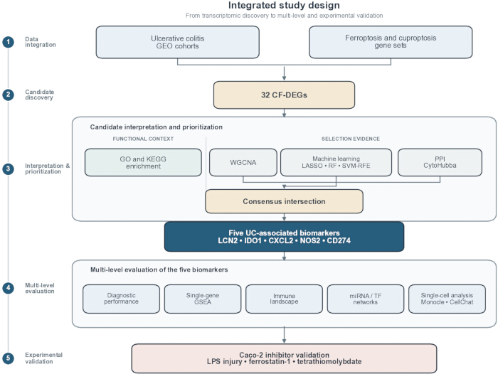
Figure 1: Study workflow. Integrated workflow for multicohort transcriptomic screening, machine-learning and network-based biomarker prioritization, single-cell localization, and inhibitor-based validation in Caco-2 cells. UC: ulcerative colitis; GEO: Gene Expression Omnibus; WGCNA: weighted gene co-expression network analysis; PPI: protein–protein interaction; ROC: receiver operating characteristic; GSEA: gene set enrichment analysis. Please click here to view a larger version of this figure.

Protocol

This study used publicly available datasets and commercially available human cell lines. No human participants, newly collected human tissue, or vertebrate animals were involved; therefore, institutional ethics committee approval was not required. Research tools, software, and online resources used in the protocol are listed in the Table of Materials.

1. Data processing for differential expression analysis

To establish the transcriptomic discovery and validation cohorts, the Gene Expression Omnibus (GEO) database was searched using the term “ulcerative colitis.” Four datasets—GSE87466, GSE92415, GSE107499, and GSE75214 were used as the training set, whereas GSE47908 was reserved for external validation. The training datasets were normalized and batch-corrected using ComBat in Sangerbox 3.0, whereas the validation dataset was processed independently.

A total of 583 ferroptosis-related genes (FRGs) were obtained from FerrDB and supplemented with genes reported in the literature to reduce single-source bias¹². A set of 96 cuproptosis-related genes (CRGs) was compiled from published studies^12,13,14. Differential expression was analyzed using limma with thresholds of |log₂ fold change| > 1 and Benjamini–Hochberg-adjusted P < 0.05. Diagnostic plots of normalization, batch correction, differential expression, and clustering are provided in Supplementary Figure 1. Sample composition, platforms, and cohort assignments are provided in Supplementary Table 1.

2. Identification of CF-DEGs in UC

Pearson correlation analysis was performed using thresholds of |r| > 0.5 and P < 0.05 to identify co-expressed FRGs and CRGs. The resulting gene set was intersected with the differentially expressed genes (DEGs) to identify cuproptosis–ferroptosis co-expressed differentially expressed genes (CF-DEGs).

3. Enrichment analysis

Gene Ontology (GO) and Kyoto Encyclopedia of Genes and Genomes (KEGG) enrichment analyses were performed using clusterProfiler and the Bioinformatics.com.cn platform. A Benjamini–Hochberg-adjusted P < 0.05 was used as the significance threshold. Enrichment plots are provided in Supplementary Figure 2.

4. Weighted gene co-expression network analysis (WGCNA)

The modular structure underlying the gene expression profiles was analyzed using weighted gene co-expression network analysis (WGCNA). Abnormal samples were identified and excluded through hierarchical clustering combined with the goodSamplesGenes function. A suitable soft-thresholding power (β) was subsequently determined to satisfy the scale-free topology criterion for network construction.

The processed expression data were used to construct a topological overlap matrix (TOM) for gene co-expression analysis. Using the dynamic tree-cutting approach, genes with highly consistent expression patterns were organized into gene modules, each containing at least 100 genes. Associations between module eigengenes (MEs) and phenotypes were analyzed to identify modules associated with the disease process and extract the corresponding gene sets. WGCNA screening diagnostics are provided in Supplementary Figure 3.

5. Selection of biomarkers

To prioritize candidates for experimental follow-up, three machine-learning algorithms were applied in parallel15. Least absolute shrinkage and selection operator (LASSO) regression was used for feature selection, random forest with ntree = 500 was used to rank gene importance, and support vector machine–recursive feature elimination (SVM-RFE) was used to identify the feature subset with the lowest cross-validation error. Full screening diagnostics are provided in Supplementary Figure 5.

Gene importance was evaluated according to the contribution of individual genes to classification accuracy, and highly ranked genes were collected to generate a preliminary gene set16. The SVM-RFE algorithm performed feature screening and model optimization through iterative feature elimination, allowing identification of the optimal feature subset for classification17. Genes shared among the three algorithms were considered candidate biomarkers identified through machine learning.

The CF-DEGs were used to construct a protein–protein interaction (PPI) network, and CytoHubba was used to rank core nodes. The intersection of key WGCNA modules, the three machine-learning outputs, and the PPI core set defined five integrated candidate biomarkers: LCN2, IDO1, CXCL2, NOS2, and CD274. These genes were classified as UC-associated diagnostic candidates. Subsequent inhibitor experiments further classified LCN2, IDO1, CXCL2, and NOS2 as ferroptosis-inhibition-responsive markers and CD274 as a cuproptosis-inhibition-responsive marker. These genes were not considered proven upstream regulators of either pathway.

6. Predictive model development and multi-method evaluation

To evaluate the clinical translational potential of the identified gene signature, a nomogram was constructed using the rms package to assess diagnostic performance. Model performance was evaluated using a calibration curve, the Hosmer–Lemeshow (HL) test, and Harrell’s concordance index (C-index).

Model calibration was assessed using the HL test and mean absolute error (MAE). A P value > 0.05 and MAE < 0.1 were established as thresholds for acceptable model fit and accuracy, respectively. Receiver operating characteristic (ROC) curves were generated, and the area under the curve (AUC) was calculated to evaluate the nomogram's predictive performance for UC. An independent dataset was used to assess model generalizability and stability.

7. Gene set enrichment analysis (GSEA)

In the training set, Spearman correlation analysis was performed between each biomarker and all other genes. The correlation results were ranked to generate an ordered gene set. Gene set enrichment analysis (GSEA) was conducted using the c2.cp.kegg_medicus.v2025.1.Hs.symbols gene set from the Molecular Signatures Database (MSigDB) as the reference. Biological pathways with P < 0.05 were considered significantly enriched.

8. Immune landscape analysis

The CIBERSORT tool and LM22 signature matrix were used to perform deconvolution analysis of the expression data and estimate the proportions of 22 immune cell subtypes. Spearman correlation analysis was subsequently performed to assess associations between the five biomarkers and immune cell subtypes.

9. Regulatory network analysis

Information on gene-related transcription factor (TF) and microRNA (miRNA) regulation was obtained from the integrated ChEA3 and TarBase 9.0 databases through the NetworkAnalyst platform. MiRNAs associated with at least two nodes were included in the regulatory network.

10. Single-cell RNA-seq

The UC single-cell datasets GSE116222, comprising three healthy and three UC samples, and GSE214695, comprising six healthy and six UC samples, were integrated. Cells were retained when they contained 200–5,000 detected genes, >1,000 unique molecular identifiers, < 30% mitochondrial transcripts, < 3% hemoglobin transcripts, and < 50% ribosomal transcripts. The NormalizeData function was used for normalization, and Harmony was used for batch correction before clustering and annotation.

After filtering, the data were normalized using the NormalizeData function. Harmony was used to minimize batch effects among samples. Uniform manifold approximation and projection (UMAP) and t-distributed stochastic neighbor embedding (t-SNE) were used for dimensionality reduction and cell clustering to characterize local and global structures within the cell population. A total of 31,712 high-quality cells were retained for further analysis. Cell types were annotated according to canonical cell marker genes.

Pseudotime analysis was performed using Monocle 2 to investigate changes in the states of epithelial and myeloid cells from UC tissues. Cell developmental trajectories and between-group differences were evaluated, and biomarker expression patterns along the pseudotime trajectory were visualized.

CellChat was used to evaluate cell–cell communication between epithelial and myeloid cell subsets. Subpopulation-specific expression patterns were integrated to infer interaction probabilities and key signaling pathways between epithelial and myeloid cells and to characterize their potential intercellular regulatory networks.

11. Cell experiments

Human Caco-2 colon adenocarcinoma cells were cultured in Dulbecco’s modified Eagle medium containing 10% fetal bovine serum, 100 U/mL penicillin, and 100 µg/mL streptomycin at 37 °C in 5% CO₂. Caco-2 cells were selected as a reproducible epithelial monolayer model for intestinal barrier and inflammatory-injury assays; however, their malignant origin limits direct generalization to nonmalignant colonic epithelium. Passage information was unavailable in the archived experimental records.

An in vitro inflammatory-injury model was established by exposing cells to 1 µg/mL lipopolysaccharide (LPS) for 24 h. Cells were assigned to a dimethyl sulfoxide vehicle-control group, an LPS-only group, an LPS + 4 µM ferrostatin-1 group, or an LPS + 40 µM tetrathiomolybdate group, with matched final solvent concentrations. The LPS-only group served as the positive injury/model control for the inhibitor-rescue comparisons.

1. Cell viability
   Cell viability was assessed using a cell viability assay according to the manufacturer’s instructions. After incubation at 37 °C for approximately 2 h, absorbance at 450 nm was measured using a microplate reader.
2. Measurement of MDA and Fe²⁺ levels
   Intracellular malondialdehyde (MDA) and Fe²⁺ levels were measured using the corresponding assay kits according to the manufacturers’ instructions. Total protein was quantified using a bicinchoninic acid assay, and each readout was normalized to the protein content of the corresponding sample.
3. Copper ion fluorescent probe assay
   After removal of the culture medium, a Cu²⁺-specific fluorescent probe was added at a final concentration of 1 µM and incubated for 30 min at 37 °C. Images were acquired immediately without washing using an inverted fluorescence microscope at excitation and emission wavelengths of 510 and 578 nm, respectively. Acquisition settings were held constant across groups, and the image scale bar was calibrated at 50 µm.
4. RT-qPCR
   Total RNA was isolated using a phenol–guanidinium-based RNA extraction reagent. Complementary DNA was synthesized from 1 µg of RNA using a first-strand complementary DNA synthesis kit, and SYBR Green-based reagents were used for real-time PCR. Each reaction was performed in technical triplicate. Primer sequences are provided in Supplementary Table 2, and relative messenger RNA abundance was calculated using the 2⁻^ΔΔCt method.

12. Statistical analysis

Normality and homogeneity of variance were assessed using the Shapiro–Wilk and median-centered Levene tests, respectively. Data meeting both assumptions were analyzed using an unpaired two-sided t-test or one-way analysis of variance followed by Tukey’s honestly significant difference test. When either assumption was not met, Welch’s t-test or Welch’s analysis of variance followed by Games–Howell comparisons was used.

Results are presented as mean ± standard deviation. Actual biological replicate counts, exact two-sided P values, and assumption checks are reported in Supplementary Table 3. The archived Figure 13 source sheet contains fewer control replicates for panels A (n = 4), C (n = 4), and F (n = 2), whereas all other panel/group combinations contain n = 6.

Computational analyses were performed using R and the limma, WGCNA, clusterProfiler, glmnet, randomForest, e1071, pROC, rms, Seurat v4, Harmony, Monocle 2, CellChat, and Cytoscape/CytoHubba workflows. Online resources included FerrDB, GEO, STRING, ChEA3, TarBase 9.0, NetworkAnalyst, CIBERSORT/LM22, MSigDB, Bioinformatics.com.cn, and Sangerbox 3.0.

Results

Identification and functional annotation of cuproptosis–ferroptosis co-expressed genes

Four training datasets comprising 421 UC samples and 97 healthy controls were integrated. A total of 551 differentially expressed genes, including 362 upregulated and 189 downregulated genes, were identified. Correlation analysis yielded 444 ferroptosis–cuproptosis-correlated genes, and intersection with the differentially expressed genes produced 32 cuproptosis–ferroptosis co-expressed diff...

Discussion

This study integrated bulk transcriptomics, machine learning, single-cell analysis, and targeted cell experiments to examine ferroptosis–cuproptosis crosstalk in UC. Five UC-associated diagnostic candidates were reproducible across discovery and validation cohorts, localized mainly to epithelial and myeloid compartments, and showed pathway-inhibition-responsive expression in Caco-2 cells. These findings support a staged workflow in which computational prioritization guides focused biological validation while avoidi...

Materials

List of materials used in this article

Name	Company	Catalog Number	Comments
BCA Protein Assay Kit	Beyotime Institute of Biotechnology	P0010	Protein quantification for normalization.
Bioinformatics.com.cn	Bioinformatics.com.cn	Online platform; accessed 2026	GO/KEGG visualization and analysis platform.
Caco-2 cell line	ATCC	HTB-37	Human colorectal adenocarcinoma cell line used for the epithelial injury model.
Cell Counting Kit-8	GLPBio	GK10001	Cell-viability assay measured at 450 nm.
CIBERSORT with LM22 signature	CIBERSORT developers	LM22	Deconvolution of 22 immune-cell fractions.
ChEA3	Ma'ayan Laboratory	Online platform; accessed 2026	Transcription-factor enrichment and regulatory-network prediction.
CO2 incubator	Not recorded	N/A	Humidified incubator used for culture at 37 °C and 5% CO2.
Cu2+ fluorescent probe	BIOFOUNT	CAS 98907-26-7	Intracellular Cu2+ fluorescence detection.
Cytoscape with CytoHubba	Cytoscape Consortium	Version not recorded	PPI visualization and core-node ranking.
Dulbecco's modified Eagle medium	Gibco	11965092	Caco-2 cell culture medium.
Dimethyl sulfoxide	Not recorded	N/A	Vehicle control.
Fetal bovine serum	Not recorded	N/A	Medium supplement at 10%.
Fe2+ Assay Kit	Abcam	ab83366	Measurement of intracellular Fe2+.
FerrDB	FerrDB developers	Online database; accessed 2026	Source of ferroptosis-related genes.
Ferrostatin-1	Sigma-Aldrich	SML0583	Ferroptosis inhibitor; final concentration 4 µM.
Harmony	Broad Institute/community	Version not recorded	Single-cell batch correction.
Inverted fluorescence microscope	Olympus	IX71	Cu2+ fluorescence imaging at 510/578 nm excitation/emission.
Lipopolysaccharide	Not recorded	N/A	Inflammatory injury stimulus at 1 µg/mL for 24 h.
Malondialdehyde Assay Kit	Beyotime Institute of Biotechnology	S0131S	Measurement of lipid peroxidation.
Microplate reader	Not recorded	N/A	Absorbance measurement at 450 nm.
Monocle	Bioconductor/community	Version 2	Single-cell pseudotime analysis.
Molecular Signatures Database	Broad Institute	c2.cp.kegg_medicus.v2025.1.Hs	Reference gene set for GSEA.
NetworkAnalyst	NetworkAnalyst developers	Online platform; accessed 2026	Integration of transcription-factor and miRNA networks.
Penicillin–streptomycin	Not recorded	N/A	100 U/mL penicillin and 100 µg/mL streptomycin.
R	R Foundation for Statistical Computing	Version not recorded	Bioinformatics analysis environment.
R package set	CRAN/Bioconductor	Package builds not recorded	limma, WGCNA, clusterProfiler, glmnet, randomForest, e1071, pROC, and rms workflows.
Real-time PCR system	Not recorded	N/A	SYBR Green RT-qPCR instrument.
RevertAid First Strand cDNA Synthesis Kit	Thermo Fisher Scientific	K1622	First-strand cDNA synthesis from 1 µg RNA.
Sangerbox	Sangerbox developers	3.0	Normalization and ComBat batch correction.
Seurat	Satija Lab/community	Version 4	Single-cell quality control, normalization, clustering, and visualization.
Statistical analysis software	Not recorded	N/A	Statistical analysis of the original cell experiments.
STRING	STRING Consortium	Online database; accessed 2026	Protein–protein interaction network construction.
SYBR Green real-time PCR reagents	Takara	RR820A	Quantitative real-time PCR.
TarBase	DIANA Tools	9.0	Experimentally supported miRNA–gene interactions.
Tetrathiomolybdate	Sigma-Aldrich	323446	Copper chelator; final concentration 40 µM.
TRIzol reagent	Takara	9108	Total RNA extraction.

References

- Fu M, Wang QW, Liu YR, Chen SJ. The role of the three major intestinal barriers in ulcerative colitis in the elderly. Ageing Res Rev. 2025;108:102752. https://doi.org/10.1016/j.arr.2025.102752.
- Le Berre C, Honap S, Peyrin-Biroulet L. Ulcerative colitis. Lancet. 2023;402:571–584.
- Wangchuk P, Yeshi K, Loukas A. Ulcerative colitis: Clinical biomarkers, therapeutic targets, and emerging treatments. Trends Pharmacol Sci. 2024;45:892–903.
- Kobayashi T, et al. Ulcerative colitis (primer). Nat Rev Dis Primers. 2020;6:74. https://doi.org/10.1038/s41572-020-0205-x.
- Huang J, et al. Comprehensive analysis of cuproptosis-related genes in immune infiltration and diagnosis in ulcerative colitis. Front Immunol. 2022;13:1008146. https://doi.org/10.3389/fimmu.2022.1008146.
- Liu Y, et al. Development and experimental validation of machine learning-based disulfidptosis-related ferroptosis biomarkers in inflammatory bowel disease. Genes. 2025;16:496. https://doi.org/10.3390/genes16050496.
- Hu W, et al. HIF-1α alleviates ferroptosis in ulcerative colitis by regulation of GPX4. Cell Death Dis. 2025;16:542. https://doi.org/10.1038/s41419-025-07883-8.
- Zhao C, et al. FXR acts as a therapeutic target for ulcerative colitis via suppressing ferroptosis. Mol Med. 2025;31:258. https://doi.org/10.1186/s10020-025-01305-3.
- Tsvetkov P, et al. Copper induces cell death by targeting lipoylated TCA cycle proteins. Science. 2022;375:1254–1261.
- Liu J, et al. Unveiling the cuproptosis in colitis and colitis-related carcinogenesis: A multifaceted player and immune moderator. Research (Wash D C). 2025;8:0698. https://doi.org/10.34133/research.0698.
- Liu N, Chen M. Crosstalk between ferroptosis and cuproptosis: From mechanism to potential clinical application. Biomed Pharmacother. 2024;171:116115. https://doi.org/10.1016/j.biopha.2023.116115.
- Hao S, et al. Development of prognostic model incorporating a ferroptosis/cuproptosis-related signature and mutational landscape analysis in muscle-invasive bladder cancer. BMC Cancer. 2024;24:958. https://doi.org/10.1186/s12885-024-12716-1.
- Wang Z, et al. Exosomes secreted by macrophages upon copper ion stimulation can promote angiogenesis. Mater Sci Eng C Mater Biol Appl. 2021;123:111981. https://doi.org/10.1016/j.msec.2021.111981.
- Zou M, Zhang W, Zhu Y, Xu Y. Identification of 6 cuproptosis-related genes for active ulcerative colitis with both diagnostic and therapeutic values. Medicine (Baltimore). 2023;102:e35503. https://doi.org/10.1097/MD.0000000000035503.
- Chen W, Miao J, Chen J, Chen J. Development of machine learning models for diagnostic biomarker identification and immune cell infiltration analysis in PCOS. J Ovarian Res. 2025;18:1. https://doi.org/10.1186/s13048-024-01582-8.
- Lv JH, et al. WGCNA combined with machine learning to find potential biomarkers of liver cancer. Medicine (Baltimore). 2023;102:e36536. https://doi.org/10.1097/MD.0000000000036536.
- Wu Q, Yang C, Huang C, Lin Z. Screening key genes for intracranial aneurysm rupture using LASSO regression and the SVM-RFE algorithm. Front Med. 2025;11:1487224. https://doi.org/10.3389/fmed.2024.1487224.
- Tang D, Pu B, Liu S, Li H. Identification of cuproptosis-associated subtypes and signature genes for diagnosis and risk prediction of ulcerative colitis based on machine learning. Front Immunol. 2023;14:1142215. https://doi.org/10.3389/fimmu.2023.1142215.
- Yang C, et al. Identification of cuproptosis hub genes contributing to the immune microenvironment in ulcerative colitis using bioinformatic analysis and experimental verification. Front Immunol. 2023;14:1113385. https://doi.org/10.3389/fimmu.2023.1113385.
- Yadav SK, et al. Fecal Lcn-2 level is a sensitive biological indicator for gut dysbiosis and intestinal inflammation in multiple sclerosis. Front Immunol. 2022;13:1015372. https://doi.org/10.3389/fimmu.2022.1015372.
- Luo Q, et al. Bioinformatics analysis reveals potential crosstalk genes and molecular mechanisms between ulcerative colitis and psoriasis. Arch Dermatol Res. 2024;317:118. https://doi.org/10.1007/s00403-024-02856-1.
- Nielsen OH, et al. Rectal dialysate and fecal concentrations of neutrophil gelatinase-associated lipocalin, interleukin-8, and tumor necrosis factor-alpha in ulcerative colitis. Am J Gastroenterol. 1999;94:2923–2928.
- Sun Y, et al. Natural polyphenol rutin inhibits ferroptosis in ulcerative colitis by regulating lipid metabolism via blocking the LCN2-ALOX15 axis. Food Funct. 2025;16:7169–7186.
- Sofia MA, et al. Tryptophan metabolism through the kynurenine pathway is associated with endoscopic inflammation in ulcerative colitis. Inflamm Bowel Dis. 2018;24:1471–1480.
- Shon WJ, et al. Severity of DSS-induced colitis is reduced in Ido1-deficient mice with down-regulation of TLR-MyD88-NF-kB transcriptional networks. Sci Rep. 2015;5:17305. https://doi.org/10.1038/srep17305.
- Zeng T, et al. Indoleamine 2, 3-dioxygenase 1 enhances hepatocytes ferroptosis in acute immune hepatitis associated with excess nitrative stress. Free Radic Biol Med. 2020;152:668–679.
- Pavlidis P, et al. Interleukin-22 regulates neutrophil recruitment in ulcerative colitis and is associated with resistance to ustekinumab therapy. Nat Commun. 2022;13:5820. https://doi.org/10.1038/s41467-022-33333-3.
- Urzua U, et al. The ovarian transcriptome of reproductively aged multiparous mice: Candidate genes for ovarian cancer protection. Biomolecules. 2020;10:113. https://doi.org/10.3390/biom10010113.
- Zahn A, et al. Transcript levels of different cytokines and chemokines correlate with clinical and endoscopic activity in ulcerative colitis. BMC Gastroenterol. 2009;9:13. https://doi.org/10.1186/1471-230X-9-13.
- Yi Q, et al. Application of genomic selection and experimental techniques to predict cell death and immunotherapeutic efficacy of ferroptosis-related CXCL2 in hepatocellular carcinoma. Front Oncol. 2022;12:998736. https://doi.org/10.3389/fonc.2022.998736.
- Kolios G, Valatas V, Ward SG. Nitric oxide in inflammatory bowel disease: A universal messenger in an unsolved puzzle. Immunology. 2004;113:427–437.
- Cheng F, et al. Identification of differential intestinal mucosa transcriptomic biomarkers for ulcerative colitis by bioinformatics analysis. Dis Markers. 2020;2020:8876565. https://doi.org/10.1155/2020/8876565.
- Tratensek A, et al. Oxidative stress-related biomarkers as promising indicators of inflammatory bowel disease activity: A systematic review and meta-analysis. Redox Biol. 2024;77:103380. https://doi.org/10.1016/j.redox.2024.103380.
- Zhang JL, et al. Jatrorrhizine alleviates ulcerative colitis via regulating gut microbiota and NOS2 expression. Gut Pathog. 2022;14:41. https://doi.org/10.1186/s13099-022-00516-7.
- Li H, et al. Development of a prognostic model based on ferroptosis-related genes for colorectal cancer patients and exploration of the biological functions of NOS2 in vivo and in vitro. Front Oncol. 2023;13:1133946. https://doi.org/10.3389/fonc.2023.1133946.
- Seibt TM, Proneth B, Conrad M. Role of GPX4 in ferroptosis and its pharmacological implication. Free Radic Biol Med. 2019;133:144–152.
- Holland T, Mattner J. Intestinal eosinophils: Characterization of elusive granulocytes as anti-bacterial and immunomodulatory effector cells in colitis. Signal Transduct Target Ther. 2023;8:321. https://doi.org/10.1038/s41392-023-01588-4.
- Nguyen J, et al. Overexpression of programmed death ligand 1 in refractory inflammatory bowel disease. Hum Pathol. 2022;126:19–27.
- Shen Z, et al. Exploration of a screening model for intrahepatic cholangiocarcinoma patients prone to cuproptosis and mechanisms of the susceptibility of CD274-knockdown intrahepatic cholangiocarcinoma cells to cuproptosis. Cancer Gene Ther. 2023;30:1663–1678.
- Niu Y, et al. Platelet activation stimulates macrophages to enhance ulcerative colitis through PF4/CXCR3 signaling. Int J Mol Med. 2025;55:78. https://doi.org/10.3892/ijmm.2025.5499.
- Qu F, et al. The role of macrophage polarization in ulcerative colitis and its treatment. Microb Pathog. 2025;199:107227. https://doi.org/10.1016/j.micpath.2025.107227.
- Danne C, Skerniskyte J, Marteyn B, Sokol H. Neutrophils: From IBD to the gut microbiota. Nat Rev Gastroenterol Hepatol. 2024;21:184–197.
- Zhao Q, et al. CD4+ T cell activation and concomitant mTOR metabolic inhibition can ablate microbiota-specific memory cells and prevent colitis. Sci Immunol. 2020;5:eabc6373. https://doi.org/10.1126/sciimmunol.abc6373.
- Chen E, et al. Inflamed ulcerative colitis regions associated with MRGPRX2-mediated mast cell degranulation and cell activation modules, defining a new therapeutic target. Gastroenterology. 2021;160:1709–1724.
- Xu H, Wu C, Wang D, Wang H. Alleviating effect of Nexrutine on mucosal inflammation in mice with ulcerative colitis: Involvement of the RELA suppression. Immun Inflamm Dis. 2024;12:e1147. https://doi.org/10.1002/iid3.1147.
- Luo Y, et al. Rab27A promotes cellular apoptosis and ROS production by regulating the miRNA-124-3p/STAT3/RelA signalling pathway in ulcerative colitis. J Cell Mol Med. 2020;24:11330–11342.
- Pace F, Watnick PI. The interplay of sex steroids, the immune response, and the intestinal microbiota. Trends Microbiol. 2021;29:849–859.
- Rodriguez J, Olivares M, Delzenne NM. Implication of the gut microbiota in metabolic inflammation associated with nutritional disorders and obesity. Mol Nutr Food Res. 2021;65:e1900481. https://doi.org/10.1002/mnfr.201900481.
- Ojha R, et al. Emerging role of circulating microRNA in the diagnosis of human infectious diseases. J Cell Physiol. 2019;234:1030–1043.
- Tian Y, et al. LncRNA CDKN2B-AS1 relieved inflammation of ulcerative colitis via sponging miR-16 and miR-195. Int Immunopharmacol. 2020;88:106970. https://doi.org/10.1016/j.intimp.2020.106970.
- Kulkarni N, Pathak M, Lal G. Role of chemokine receptors and intestinal epithelial cells in the mucosal inflammation and tolerance. J Leukoc Biol. 2017;101:377–394.
- Stadnyk AW. Intestinal epithelial cells as a source of inflammatory cytokines and chemokines. Can J Gastroenterol. 2002;16:241–246.
- Xu Y, Chen N. DUOX2-mediated innate immune hyperactivation drives macrophage M1 polarization via the APP-CD74 axis in inflammatory bowel disease. Presented at: 19th Congress of the European Crohn’s and Colitis Organisation (ECCO 2026); Stockholm, Sweden; 2026. https://academic.oup.com/ecco-jcc/article/20/Supplement_1/jjaf231.232/8432779.
- Shi CL, et al. Single-nucleus transcriptome unveils the role of ferroptosis in ischemic stroke. Heliyon. 2024;10:e32727. https://doi.org/10.1016/j.heliyon.2024.e32727.
- Tu H, et al. Integrated single-cell analysis with experimental validation reveals ANXA2 as a therapeutic target for ferroptosis in inflammatory bowel disease. Am J Transl Res. 2026;18:91–111.
- Yan C, et al. Exploring the anti-ferroptosis mechanism of Kai-Xin-San against Alzheimer's disease through integrating network pharmacology, bioinformatics, and experimental validation strategy in vivo and in vitro. J Ethnopharmacol. 2024;326:117915. https://doi.org/10.1016/j.jep.2024.117915.
- Shaik JP, Ahmad A. Pharmacological mechanism of cinnamic acid in the treatment of prostate cancer by network pharmacology. Archives of Medical Reports. 2024;1(2):1–6. https://doi.org/10.26524/amr.2024.2.1.
- Nimmagadda S, Patel S, MR Vishwathika. Targeting ferroptosis: A novel therapeutic avenue in osteoarthritis and bone degeneration. Archives of Medical Reports. 2025;2(5):6–9. https://doi.org/10.26524/amr.2025.5.2.
Access restricted. Please log in or start a trial to view this content.