A Stochastic Optimal Semi-active Control method with time delay compensation (SOSC-PSO) is proposed in this paper, which is designed to maintain the reliability of structures controlled by MR dampers.
A subscription to JoVE is required to view this content. Sign in or start your free trial.
Research Article
Stochastic Semi-active Control Method of Structure Based on Magnetorheological Dampers Considering Time Delay
In This Article
Summary
Abstract
The use of Magnetorheological (MR) dampers in semi-active control systems faces a key challenge: time delay caused by feedback processes, which reduces the reliability of civil engineering structures under stochastic excitations. This paper proposes a Stochastic Optimal Semi-active Control method with time delay compensation (SOSC-PSO), leveraging the Physical Stochastic Optimal control theory (PSO) to address this issue and maintain structural reliability. The proposed method derives the semi-active control force as a function of both current and previous states, compensating for time delays in the control process. To optimize control effectiveness, key parameters are tuned based on a reliability criterion for the system. Validation analyses on single-degree-of-freedom and multi-degree-of-freedom structures under stochastic seismic excitations show that time delays significantly impair the performance of MR dampers. However, the SOSC-PSO method with time delay compensation significantly improves control effectiveness, and with optimized parameters, it enhances the reliability of the structural control system beyond methods without parameter optimization.
Introduction
Improving the performance of engineering structures in the face of catastrophic events, such as earthquakes and extreme winds, remains a primary concern within the civil engineering community. Structural control, an effective technique for reducing vibrations, has been proven to enhance both the safety and functionality of such structures1,2,3. Over the past few decades, various advanced methods and technologies have been developed for this purpose. These methods can be broadly classified into four categories based on the type of energy used to drive the control devices: active, semi-active, passive, and hybrid control systems4,5,6,7.
In active control, the required control force is directly applied through the control devices, which necessitates a significant amount of energy8,9,10. Semi-active control, on the other hand, involves adjusting the properties of control devices (such as damping or stiffness) based on control signals, requiring much less energy compared to active systems11. Passive control, in contrast, relies on energy dissipation without any external energy input into the system12,13,14. Hybrid systems combine the features of active/semi-active and passive control strategies to achieve more effective performance15. Among these approaches, semi-active control is considered particularly promising due to its balance of low energy consumption and high efficiency16,17,18. The magnetorheological (MR) damper, with its superior dynamic damping characteristics, is regarded as one of the most effective semi-active control devices19,20,21,22.
However, a challenge arises in semi-active control systems that utilize MR dampers, as feedback logic inevitably introduces time delays. These delays are typically caused by several factors23,24,25, including: (i) the acquisition and processing of sensor data, (ii) the computation of the required control force by the controller26, (iii) signal transmission through transducers to the MR dampers27, and (iv) the actual force generation by the MR dampers themselves28. Such time delays can lead to discrepancies between the control force produced and the force expected by the structure, significantly compromising the control effectiveness29. Unfortunately, most existing control algorithms for MR dampers do not account for these delays.
Additionally, due to the inherent randomness of catastrophic events, any effective semi-active control algorithm must be able to maintain performance under stochastic excitations. The Linear Quadratic Gaussian (LQG) control method, a classical stochastic optimization technique, has been explored for mitigating vibrations in structures equipped with MR dampers. For example, Dyke et al. proposed an LQG clipped-optimal control strategy for improving the seismic response of structures fitted with MR dampers, using acceleration feedback30. Ying et al. introduced a non-clipped semi-active stochastic optimal control strategy for nonlinear structures with MR dampers, incorporating stochastic averaging and dynamic programming techniques31. Other studies have applied modal-based LQG control to enhance the seismic performance of base-isolated buildings19 and analyzed its effectiveness for vibration mitigation in wind turbine towers32. However, classical LQG methods, which assume white Gaussian noise, are not well-suited for modeling the non-stationary, non-Gaussian nature of real-world excitations like earthquakes or strong winds. To address this, the concept of physically-based stochastic optimal (PSO) control has been developed33,34, which overcomes the limitations of traditional LQG methods and offers a more accurate framework for handling diverse stochastic excitations35. Studies have shown that PSO-based semi-active stochastic optimal control significantly improves vibration mitigation for both linear and nonlinear structures subjected to stochastic seismic forces36.
Thus, there is an urgent need for a robust semi-active control method that compensates for time delays, enhancing the reliability of structures controlled by MR dampers25,37. Furthermore, to ensure optimal control performance under stochastic excitations, it is essential to optimize the critical parameters of the proposed control method using a reliability-based approach. Therefore, a Stochastic Optimal Semi-active Control method with time delay compensation (SOSC-PSO) is proposed in this paper to improve the reliability of structures with MR dampers.
Access restricted. Please log in or start a trial to view this content.
Protocol
1. Stochastic optimal semi-active control method
As the control effect of an MR damper is significantly influenced by the inevitable time delay, a semi-active control method with a time delay compensation algorithm is developed to increase the performance of the controlled structure. Besides, the randomness inherent in external excitations causes the obvious uncertainties of dynamic responses. The PSO control is introduced to optimize the critical parameters of the proposed method for ensuring the reliability of structure control system.
1.1 Compensation algorithm of semi-active control
Without loss of generality, consider an n-Degree-Of-Freedoms(n-DOF) structure controlled by MR dampers with time delay, of which the motion equation subjected to stochastic excitations is given by:
 (1)
(1)
Where  represent the n x n mass, damping, and stiffness matrices of the structure, respectively; n represents the number of degrees of freedom of the controlled structure. The displacement, velocity, and acceleration vectors of structure are represented by
  , respectively. The small one and two dots above the symbols represent the first- and second-time derivatives. Us (t - tD) represents the r-dimensional vector of the time-delayed control force of MR dampers, and r represents the number of dampers; t represents the time; tD denotes time delay, assumed to be uniform across all dampers in this study, where
  , with here the integral number
  , and
, and  denoting the sampling period.
  represents the p-dimensional vector of stochastic excitations, and
  represents the stochastic parameter vector characterizing the randomness associated with external excitations. The dimension of depends on the model used for the external excitations but is not related to the mechanical degrees of freedom of the structure. Bs and D are n x r and n x p matrices that specify the locations of the dampers and external excitations, respectively. In the state-space representation, Eq. (1) is written as:
 (2)
(2)
Where  represents 2n-dimensional state vector;
  represents 2n x 2n system matrix;
  represents 2n x r location matrix of MR dampers;
  represents 2n x p location matrix of external excitations. These parameters are expressed as:
![Dynamic system state vector equation; z=[X(t), Ẋ(t)]; mathematical representation.](/files/ftp_upload/68259/68259eq028.jpg "figure-protocol-15") ,
,  ,
, 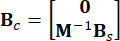 ,
, ![Matrix manipulation equation, showing Dc = [0; M⁻¹D] for computational modeling.](/files/ftp_upload/68259/68259eq031.jpg "figure-protocol-18") (3)
(3)
Where  denotes an identity matrix with the same order of
  . For the convenience of calculation, the continuous state space equation Eq. (2) can be expressed in discrete form as:
 (4)
(4)
Where the time point  is simplified as
  . And
. And  ,
,  ,
,  denote 2n x 2n, 2n x r and 2n x p matrices, which are expressed as:
 ,
,  ,
,  (5)
(5)
Where  denotes the sampling period.
To achieve similar effectiveness as the active control, a simple and efficient control method based on the Hrovat algorithm38 is proposed for the MR damper based control with time delay:
 (6)
(6)
where  represents the semi-active control force signal at time point\ for the MR damper;
  represents the reference active control force with time delay compensation;
  represents the maximum damping force of the MR damper, which is changeable;
  represents the absolute value operation symbol;
  represent the maximum and minimum Coulombic forces of MR damper;
  represents the viscous damping coefficient;
  represents the velocity input in MR damper, which is the motion velocity of piston relative to the damper cylinder. In Eq. (6),
  represent the designed parameters of the MR damper.
Eq. (6) shows the calculation of the semi-active control force of the MR damper with time delay. It is seen that the semi-active control force  , at time step
  in Eq. (4), is calculated based on the active control force
  at time step and state variable
  at time step
  since the
  time steps delay. To obtain the active control force , the conventional cost function is established by
 (7)
(7)
Where  represents the 2n x 2n symmetric positive semi-definite weighting matrix of the system state;
  represents the r x r symmetric positive definite weighting matrix of the control force. It is seen that the external excitation is negligible. Actually, based on Eq. (7), the structure control system can achieve the optimal control effect whatever the kind of external excitation. As the discrete form, Eq. (7) is expressed as39:
 (8)
(8)
The minimization of the cost function  leads to a conditional extreme-value problem, and the active control force
  is calculated by25:
 (9)
(9)
Where  denote the control gains for the state variable
  at time step and active control force
  at time step
  , which is determined by the weighting matrices
  and
and  37. Since the inevitable time delay, the obtained control force
  are acted on the structure at time points
  . Therefore, the active control force in Eq. (9) is calculated by:
 (10)
(10)
For the clarity of conception, the semi-active control force in Eq. (10) is expressed as follows based on Eq. (6):
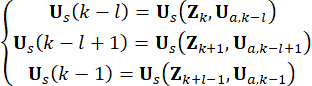 (11)
(11)
Where  denotes the active control force at time point
  . Substituting Eq. (11) into Eq. (10),
 (12)
(12)
NOTE: All the state  values from time point to
  are needed for calculating . Therefore, the following state prediction method is introduced40.
 (13)
(13)
Where  denotes the predicted variable. By the iteration of Eq. (13), the state at
  is calculated. Active control force Ua(k) is expressed as:
 (14)
(14)
The semi-active control force can be obtained by combining Eqs. (6), (12), and (13).
1.2 Reliability analysis of the structure control system
According to the principle of probability preservation, the augmented system  and
and  of structure with MR dampers are probability-conserved, and they are governed by the following generalized probability density evolution equations (GDEEs)38:
 (15)
(15)
 (16)
(16)
Where , denote the corresponding components of the system state and semi-active control force with time delay, respectively;  and
and  denote the joint probability density functions of augmented sample systems
  and
and  , respectively;
  denotes the sample within the sample space of ;
  and
and  ) denote the first-order time partial derivatives of system state and semi-active control force components, respectively. The joint probability density functions
  and can be achieved by solving Eqs. (15) and (16) with the following initial conditions:
 (17)
(17)
 (18)
(18)
Where  denotes the Dirac delta function;
  and
and  denote the deterministic initial values of
  and
and  , respectively;
  denotes the probability density function of sample
  .
.
The instantaneous probability density functions of and can be obtained by the one-dimensional integration of and over the domain of sample space:
 (19)
(19)
 (20)
(20)
Where  denotes the distribution domain of .
Based on Eqs. (19) and (20), it is seen that the complete probabilistic information of the concerned physical quantities are readily derived, if their relationships associated with algorithm parameters are defined. The reliability of concerned physical quantities can be calculated by the following pertinent performance function:
 (21)
(21)
 (22)
(22)
Where  and
and  denote the calculated reliability of the concerned state quantity and semi-active control force, respectively;
 ![Mathematical formula for maximizing function; Z̄i=max [ max|Wik(Θ,t)| ]; used in data analysis.](/files/ftp_upload/68259/68259eq117.jpg "figure-protocol-116") denotes the equivalent extreme-value vector of the i-th concerned physical quantity of the controlled structure;
denotes the equivalent extreme-value vector of the i-th concerned physical quantity of the controlled structure;  denotes the equivalent extreme-value vector of the j-th control force; the hat ‘-’ on symbols indicates the equivalent extreme-value vector41;
  denotes the i-th concerned physical quantity of the k-th DOF of controlled structure;
  denotes the j-th control force;
  ,
,  ,
,  ,
, ,
,  and
and  denote the number of concerned physical quantities and DOF of the structure and MR dampers installed in the structure, respectively.
  and
and  denotes the thresholds of
  and
and  ;
;  denotes the probability of the random event.
1.3 Optimization of parameters
The ratio of the amplitudes of and highly influences the control effectiveness38 in the feedback control modality. Therefore, to achieve the best control effectiveness, and need to be optimized. Besides, as an MR damper-based control method, the control effectiveness is also impacted by the device parameters, in Eq. (6). For achieving the optimal reliability of the structure control system, the reliability-based criterion is proposed in Eq. (25).
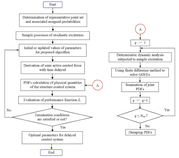
Figure 1: Flowchart of parameter optimization for stochastic optimal semi-active structure control with time delay compensation. Abbreviations: GDEE = Generalized Differential Equation of the Event ; PDF = Probability Density Function. Please click here to view a larger version of this figure.
In summary, two stages are required to carry out the stochastic optimal semi-active structure control based on MR dampers with time delay compensation:
1.3.1 Minimizing the cost function  shown in Eq. (7), the state feedback logic in the sense of samples is achieved, that is, Eq. 12)
1.3.2 Minimizing reliability-based performance function  ,the optimal parameters in the sense of statistics are achieved. Figure 1 presents the optimization flowchart of the controller’s parameters in step 1.3.2.
The following steps in step 1.3.2, which involve two layers of loops, are as follows:
1.3.2.1 Partitioning the probability-assigned space of stochastic excitations, which is characterized by the stochastic parameter vector  , allows for the identification of a set of representative points
  along with their associated assigned probabilitiesPq’s. This approach enables the efficient generation of sample processes for the stochastic excitation, denoted as
 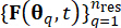 , to be readily obtained.
1.3.2.2 For the parameter optimization of the semi-active structure control system, initialize or update the values of cost-function weights and . The associated state feedback control force with time delay, see Eq. (12), is then calculated.
1.3.2.3 Obtaining the probability density functions (PDFs) of structural responses and control force by solving the GDEEs shown in Eqs. (17)–(20):
The optimization is offline completion but not online. In the applicable of proposed method in real structure control systems, the optimal and have been achieved, and the optimization isn’t needed in the real applicable process.
Deterministic dynamic analysis of the semi-active structure control system subjected to sample excitation, by which the concerned physical quantities  and their derivatives
  are calculated.
By employing a finite difference method, such as the modified Lax-Wendroff scheme with Total Variation Diminishing(TVD) properties, the Generalized Differential Equations (GDEEs) can be solved, and numerical solutions for the joint probability density functions  , can be derived.
Repeating the above two steps of deterministic dynamic analysis and finite difference method, and running over all the representative points  , the probability density functions can be obtained by summation:
 (23)
(23)
 (24)
(24)
Where  represents the area measure of the subdomain associated with the sample point
  . The method used to solve the Generalized Differential Equation of the Event (GDEE) is known as the probability density evolution method (PDEM)42.
1.3.2.4 The PDFs of the relevant physical quantities are used to assess their reliability, which are then incorporated into the performance function of the probabilistic criterion.
1.3.2.5 Evaluate whether the termination criteria for the parameter optimization process have been met. If the conditions are not satisfied, return to Step 1.3.2.2; if they are, the optimal parameters for the time-delayed control system can be determined. In this work, the genetic algorithm (GA) toolbox in MATLAB is used for parameter optimization, which facilitates parameter updates and defines the termination conditions. By genetic algorithm, the optimal values can be achieved within ten iterations, and the convergence is stable without local minima problems. Although the computational cost of GA is larger than particle swarm optimization or gradient-based methods, the GA is good at dealing with complex and non-differentiable problems, such as the one in this manuscript. Therefore, the GA is applied. And since the rapid convergence property, the computational cost of GA is acceptable.
1.3.2.6 To achieve optimal reliability control, the following performance function is formulated.Minimize to determine the optimal values of parameters  and
and  :
:
 } (25)
 (26)
(26)
As previously mentioned, the weighting matrices of the controller are symmetric, where the elements in matrix correspond to the weights assigned to displacement, velocity, and their interaction, while the elements in matrix represent the weights related to the control force. Based on the findings from earlier studies38, it has been observed that varying the configurations of the cost-function weights and has minimal impact on control effectiveness. Consequently, a simplified configuration is adopted in this study, as outlined below:
![Matrix equations, Q = q · [K 0; 0 M], linear algebra, matrix operations, educational formula.](/files/ftp_upload/68259/68259eq153.jpg "figure-protocol-165") ,
,  (27)
(27)
Where  denotes the coefficient of the state weighting matrix to be defined;
  denotes the coefficient of the control weighting matrix to be defined;
  denotes the identity matrix. The control effect is influenced by the ratio of to but not the values themselves. Besides,
  in Eq. (6) denotes the minimum Coulombic force of the MR damper, which means that
  with the current input in the damper being zero. Then, Eq. (26) can be further expressed as:T
 (28)
(28)
Where  are the optimal coefficients of concern. To make them reasonable in engineering, the optimal ranges of them are based on the production capacity of the MR damper factories.
Obviously, the optimal parameters obtained by Eq. (28) maintain the optimal control effectiveness of the proposed semi-active control algorithm with time delay, which enables the structure control system to achieve the balanced optimal reliability subjected to stochastic excitations.
2. Case study
To analyze the effectiveness of the proposed semi-active control method with time delay compensation for an MR damper, a planar single-story shear frame structure attached to an MR damper was subjected to the horizontal stochastic seismic ground motion, as shown in Figure 2. The parameters of the semi-actively controlled structure system are as follows: structure mass  , natural circular frequency
  , damping ratio
  . According to past experience and existing damper scales in the market, the threshold values of structural displacement, velocity, acceleration, and control force are 10 mm, 100 mm/s, 1,500 mm/s2, and 150 kN, respectively. For representing the stochastic seismic ground motion, the physically motivated stochastic ground motion model was employed43:
 (29)
(29)
Where  represents the ground motion in the time domain at the engineering site, and
  denotes the ground motion in the frequency domain at the bedrock. The vector
  characterizes the stochastic nature of the ground motion at the surface of the engineering site. The parameters
  are stochastic variables that describe the characteristics of the site soil, including the predominant frequency
  and the equivalent damping
  . The vector
  represents the stochastic nature of the ground motion at the bedrock, which is influenced by source properties and the propagation path, with
  indicating the number of stochastic variables involved at this stage.
  refers to the circular frequency, and i is the imaginary unit.
The predominant frequency  and the equivalent damping ratio of the engineering site are key parameters that characterize the dynamic properties of the site soil. The probabilistic distribution and statistical parameters of these quantities can be determined based on seismic acceleration records collected from a specific class of engineering sites. For illustrative purposes, a site class with a shear-wave velocity range of [150, 250] m/s was considered, and the design characteristic period of the ground motion was set to 0.45 s.
The critical parameters , were treated as mutually independent stochastic variables, both following a log-normal distribution for parameter identification. The statistical parameters were as follows: the means of , were 12 rad/s and 0.1, respectively. The coefficients of variation of and were 0.42 and 0.35, respectively. The ground motion at the bedrock was modeled as a Gaussian white noise process with a Fourier amplitude of 0.20 m/s2, corresponding to a peak ground acceleration of 0.11 g. The phase angle used to generate the bedrock motion was denoted as  . Therefore, Sb =1 and
  . This approach can be considered as modeling conditional stochastic ground motions with a given exceedance probability44. The assumption of log-normal distribution is widely used in ground motion modeling due to its ability to capture the skewed nature of observed ground motion parameters.
To assess the sensitivity of this assumption, the additional analyses using alternative probabilistic distributions, including the normal and gamma distributions have been conducted in other researches45,46. The findings indicate that while the overall trends remain consistent, the log-normal distribution provides the best fit to the observed data, particularly for capturing the tail behavior of ground motion intensity measures
By virtue of the tangent spheres method47, a collection of 221 representative points with associated assigned probabilities was selected and representative ground accelerations were synthesized. The sampling frequency was 50 Hz, and the duration of the ground motions was 20.48 s. To assign a non-stationary intensity to the simulated ground motion, a uniform modulation function was utilized and its formulation was as follows42:
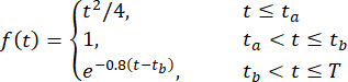 (30)
(30)
Where  take 2 and 16 s, respectively.
The mean and standard deviation of the stochastic seismic ground motion, and a time history of representative seismic ground motion are shown in Figure 3. The amplitude of the mean (0.06 m/s2) was ~8% of the amplitude of the standard deviation (0.8 m/s2), indicating that the physically motivated stochastic ground motion model exhibited the property of zero mean. Meanwhile, the seismic ground motion exhibited remarkable non-stationary behaviors both in temporal and frequency domains.
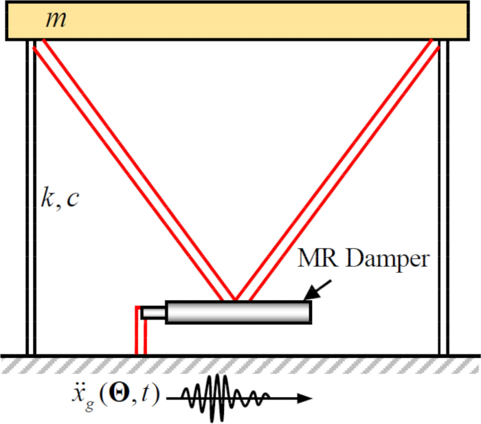
Figure 2: Sketch of a single-story shear frame with a magnetorheological damper.  denote structure mass, damping ratio and stiffness;
  denotes the stochastic seismic excitation. Please click here to view a larger version of this figure.
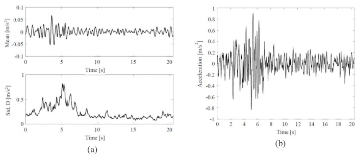
Figure 3: Statistics and representative samples of selected seismic ground motions. (A) Mean and standard deviation of stochastic seismic ground motion; (B) Time history of representative seismic ground motion. Please click here to view a larger version of this figure.
2.1 Influence analysis of time-delay
To analyze the influence of time delay on the semi-active control effectiveness of an MR damper, Figure 4 shows the displacement, velocity, and acceleration RMS (root-mean-square response) of the controlled structure. The weighting matrix ratio and damper parameters were  ,
,  , and
, and  , which are the optimized results without time delay38. The responses of the controlled structure with time delay were larger than the controlled structure without time delay, and the influence of time delay on the control effect represented periodicity along with the time delay increasing. Since the semi-active control method with an MR damper is a kind of feedback method, the periodicity of the influence was considered to be related to the natural period of the controlled structure (T = 0.56 s).
Compared with the responses of uncontrolled structure, of which the maximum MRS displacement, velocity, and acceleration were 24.6 mm, 270.0 mm/s, and 3111.3 mm/s2, the MR damper-controlled structure achieved a notable effect. Unlike the instability of the active controlled structure with time delay25, the MR damper-based semi-active control method still obtained some effect even with time delay.
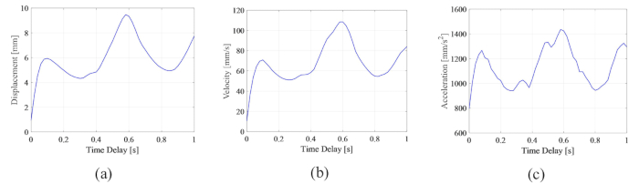
Figure 4: The maximum root-mean-squares of the controlled structure's responses with time. (A) Displacement; (B) Velocity; (C) Acceleration. Please click here to view a larger version of this figure.
To analyze the influence of time delay on the reliability of a semi-actively controlled structure, Figure 5 shows the reliability of displacement, velocity, and acceleration with increasing time delay. The reliability of controlled structure responses with any time delay was lower than the values without time delay, which means that the reliability of the controlled structure was decreased by time delay. Meanwhile, similar to the maximum RMS, the reliability control effect showed periodicity with increasing time delay. Further, the reliability of the controlled structure, with or without time delay, was higher than the values of uncontrolled structures with reliability of displacement, velocity, and acceleration 0.0954, 0.1058, and 0.1111.
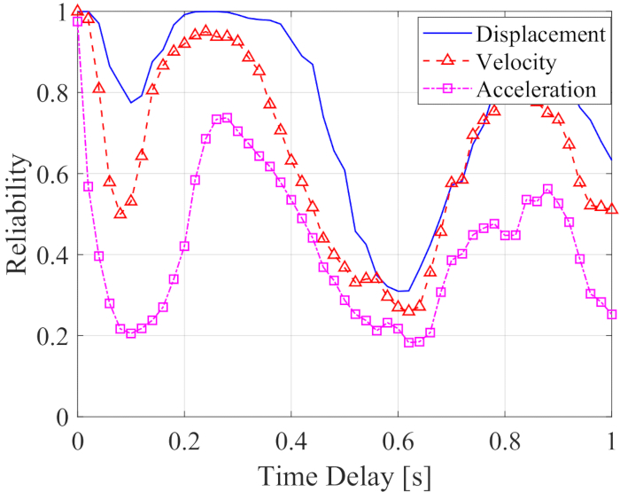
Figure 5: Responses' reliability of controlled structure with increasing time delay. Please click here to view a larger version of this figure.
In summary, the responses of the structure were mitigated by the semi-active control method. However, the control effectiveness, regardless of the RMS or reliability, of the semi-active control method was decreased by time delay. Therefore, it is necessary to compensate for the time delay.
2.1.1 Analysis of the time delay compensation method
For analyzing the effectiveness of the proposed time delay compensation method, the RMS time histories of displacement, velocity, and acceleration for uncontrolled (Unc), time-delayed system with non-compensation controlled (TDN-SAC-PSO), and time-delayed system with compensation controlled (TDC-SAC-PSO) are compared in Figure 6, where the time delay was 0.1 s. The parameters of the weighting matrix and the semi-active control method are the same as in step 2.1.
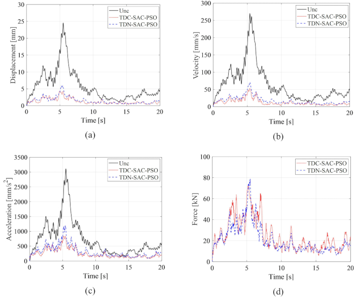
Figure 6: Root-mean-square time history comparison of structures controlled by different methods. (A) Displacement; (B) Velocity; (C) Acceleration; (D) Control force. Abbreviations: Unc = uncontrolled; TDC-SAC-PSO = time delayed system with compensation controlled; TDN -SAC-PSO = time delayed system with non-compensation controlled. Please click here to view a larger version of this figure.
Both the control methods significantly decreased the responses of the structure compared with the uncontrolled structure, revealing the advantages of the MR damper-based control method. Compared with the uncontrolled structure, the maximum RMS of displacement, velocity, and acceleration are decreased by 75.79%, 73.75%, and 61.22% with the TDN-SAC-PSO method. Further, with the time delay compensation, the responses of the controlled structure are decreased by 82.59%, 80.40%, and 73.04% with the TDC-SAC-PSO method. The maximum RMS of the control force with the TDC-SAC-PSO method decreased by 8.43% compared to the TDN-SAC-PSO method, although the vibration responses of the former method were less than the latter. The above analysis indicates that the influence of time delay on the MR damper-based control method was effectively decreased by the compensation method, which shows the necessary of time delay compensation for MR damper semi-active control method.
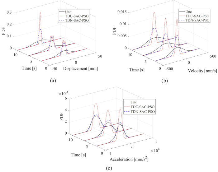
Figure 7: PDF comparison at typical times of structure responses. (A) Displacement; (B) Velocity; (C) Acceleration. Abbreviations: PDF = probability density function; Unc = uncontrolled; TDC-SAC-PSO = time delayed system with compensation controlled; TDN -SAC-PSO = time delayed system with non-compensation controlled. Please click here to view a larger version of this figure.
To comprehensively reveal the effect of the proposed compensation method on the uncertainty of the responses of the controlled structure, the probability density function (PDF) comparisons of displacement, velocity, and acceleration at typical times, 3, 7 and 11s, are shown in Figure 7. The PDFs for the TDN-SAC-PSO method were narrower than those of the Uncontrolled structure, which means that the uncertainty of the structure responses was decreased by the semi-actively control method even with time delay. When the time delay was compensated, the PDFs of the responses were further narrowed. Therefore, the proposed compensation method is necessary for improving the semi-active control effect.
| Control method | Displacement | Velocity | Acceleration | Control Force | Minimum value |
| Unc | 0.0954 | 0.1058 | 0.1111 | -- | 0.1111 |
| TDC-SAC-PSO | 0.9565 | 0.8107 | 0.7654 | 0.9845 | 0.7654 |
| TDN-SAC-PSO | 0.7747 | 0.531 | 0.2054 | 0.884 | 0.2054 |
Table 1: Vibration responses and control force reliability of structures controlled by different methods. Abbreviations: Unc = uncontrolled; TDC-SAC-PSO = time delayed system with compensation controlled; TDN -SAC-PSO = time delayed system with non-compensation controlled.
The vibration responses and control force reliability of Uncontrolled, TDC-SAC-PSO-, and TDN-SAC-PSO method-controlled structures are shown in Table 1. With the TDN-SAC-PSO method control, the reliability of the structure was dramatically increased compared with the Uncontrolled structure, which validates the effectiveness of the MR damper-based control method, even with time. However, with time delay compensation, the reliability was significantly increased compared to without compensation, especially for the acceleration. It is also noteworthy that the reliability of different responses and the control force showed significant differences for the TDC-SAC-PSO method. This indicates that the optimal values of critical parameters for the control without time delay are not optimal for the control with time delay. To achieve the optimal control effect of the vibration responses and control force with time delay influence, the parameters need to be optimized further. Based on the above analysis, it is concluded that the semi-active control method with an MR damper can effectively decrease the vibration responses of the structure, while the parameters need to be optimized because of the influence of time delay.
2.2 Parameter optimization
To achieve the optimal values of the parameters, the integrated optimization method based on the reliability criterion was applied38. The optimization of critical parameters was carried out with  ,
, ![Static equilibrium, formula r ∈ [10^-20, 10^-1], mathematical expression in scientific research.](/files/ftp_upload/68259/68259eq186.jpg "figure-protocol-213") ,
, ![Damping coefficient range equation, c_D ∈ [0.2,2] kN·s/mm, related to mechanical analysis.](/files/ftp_upload/68259/68259eq187.jpg "figure-protocol-214") ,
, ![Maximum static load equation \( U_{dc,max} \in [50,150] \) kN, structural analysis formula.](/files/ftp_upload/68259/68259eq188.jpg "figure-protocol-215") , and the tunable times of the MR damper force s = 8. The GA toolbox within MATLAB was used to implement the optimization.
, and the tunable times of the MR damper force s = 8. The GA toolbox within MATLAB was used to implement the optimization.
The optimization results of the parameters are  ,
,  , and
, and  for the time delay
  . Figure 8 shows the RMS time histories of displacement, velocity, acceleration, and control force for the Uncontrolled (Unc), TDC-SAC-PSO method- and SOSC-PSO method-controlled structures. The SOSC-PSO method denotes the semi-active control method with time delay compensation and optimized critical parameter values.
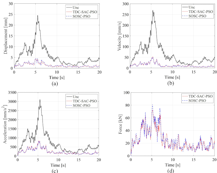
Figure 8: RMS time histories of displacement, velocity, acceleration, and control force for Uncontrolled and TDC-SAC-PSO method- and SOSC-PSO method-controlled structures. (A) Displacement; (B) Velocity; (C) Acceleration; (D) Control force. Abbreviations: Unc = uncontrolled; TDC-SAC-PSO = time delayed system with compensation controlled; SOSC-PSO = Stochastic Optimal Semi-active Control method with time delay compensation. Please click here to view a larger version of this figure.
From Figure 8, it is seen that the control effects of the TDC-SAC-PSO and SOSC-PSO methods showed little difference. The maximum RMS of the displacement velocity and acceleration for the former method were 81.60%, 81.21%, 73.62% of the uncontrolled structure and 82.59%, 80.40%, 73.04% for the latter method. To comprehensively analyze the probability characteristics of the responses for both control methods, Figure 9 shows the PDFs of displacement, velocity, and acceleration for the Uncontrolled, TDC-SAC-PSO method- and SOSC-PSO method-controlled structures. Both the control methods had almost the same PDFs of displacement and velocity at typical times. The acceleration PDFs of the SOSC-PSO method were narrower than those of the TDC-SAC-PSO method, which means that the uncertainty of acceleration achieved a better control effect by the former method.
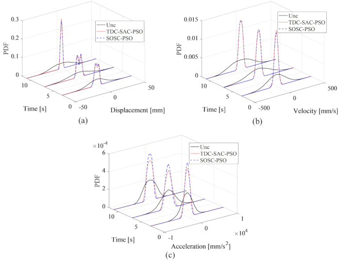
Figure 9: PDFs comparison of displacement, velocity, and acceleration for different controlled structures. (A) Displacement; (B) Velocity; (C) Acceleration. Abbreviations: PDFs = probability density functions; Unc = uncontrolled; TDC-SAC-PSO = time delayed system with compensation controlled; SOSC-PSO = Stochastic Optimal Semi-active Control method with time delay compensation. Please click here to view a larger version of this figure.
The reliability of displacement, velocity, acceleration, and control force for the uncontrolled and TDC-SAC-PSO- and SOSC-PSO method-controlled structures are shown in Table 2. Both the control methods achieved significant increase in reliability compared with the uncontrolled structure. The displacement reliability showed little difference between the TDC-SAC-PSO and SOSC-PSO methods. While the acceleration reliability, the lowest reliability of the controlled structure, achieved a noticeable increase. It means that the SOSC-PSO method achieves the balance optimal control effect.
| Control method | Displacement | Velocity | Acceleration | Control force | Minimum value |
| Unc | 0.0954 | 0.1058 | 0.1111 | -- | 0.1111 |
| TDC-SAC-PSO | 0.9565 | 0.8107 | 0.7654 | 0.9845 | 0.7654 |
| SOSC-PSO | 0.953 | 0.8704 | 0.8934 | 0.9586 | 0.8934 |
Table 2: Reliability for structures controlled by different methods. Abbreviations: Unc = uncontrolled; TDC-SAC-PSO = time delayed system with compensation controlled; SOSC-PSO = Stochastic Optimal Semi-active Control method with time delay compensation.
The effectiveness of the proposed SOSC-PSO method with time delay was analyzed. To further verify the proposed method for different time delays, Table 3 shows the optimal parameter values and corresponding reliability for the time delay range ![Static equilibrium equation, \( t_D \in [0,0.3]s \), mathematical expression for analysis.](/files/ftp_upload/68259/68259eq194.jpg "figure-protocol-223") .
.
| tD(s) | lg(r*) | CD(kN·s/mm) | Udc,max (kN) | Displacement | Velocity | Acceleration | Control force |
| 0 | -2.524 | 1.44 | 116.163 | 0.9997 | 0.9998 | 0.9752 | 1 |
| 0.02 | -4.413 | 0.414 | 144.066 | 0.9989 | 0.9988 | 0.872 | 0.9011 |
| 0.04 | -4.416 | 0.25 | 141.759 | 0.9998 | 0.9846 | 0.8881 | 0.9135 |
| 0.06 | -3.226 | 0.203 | 145.613 | 0.993 | 0.9318 | 0.8756 | 0.9556 |
| 0.08 | -5.207 | 0.345 | 133.692 | 0.9646 | 0.8998 | 0.8998 | 0.953 |
| 0.1 | -4.669 | 0.702 | 130.739 | 0.9531 | 0.8704 | 0.8934 | 0.9586 |
| 0.12 | -4.895 | 0.833 | 69.72 | 0.9526 | 0.863 | 0.888 | 0.9686 |
| 0.14 | -4.231 | 0.921 | 75.221 | 0.9531 | 0.8681 | 0.8697 | 0.9671 |
| 0.16 | -5.594 | 0.662 | 138.922 | 0.9529 | 0.8461 | 0.8262 | 0.931 |
| 0.18 | -4.262 | 0.882 | 76.335 | 0.9516 | 0.7873 | 0.7614 | 0.9618 |
| 0.2 | -3.926 | 0.783 | 67.951 | 0.904 | 0.7277 | 0.7116 | 0.9653 |
| 0.22 | -5.965 | 1.071 | 52.554 | 0.8377 | 0.6411 | 0.6205 | 0.965 |
| 0.24 | -4.481 | 1.216 | 128.148 | 0.7567 | 0.474 | 0.474 | 0.9687 |
| 0.26 | -3.53 | 0.672 | 53.706 | 0.53 | 0.4096 | 0.4158 | 0.9921 |
| 0.28 | -4.433 | 0.638 | 64.225 | 0.3547 | 0.3745 | 0.3464 | 0.9928 |
| 0.3 | -3.536 | 0.459 | 57.705 | 0.2735 | 0.316 | 0.2736 | 0.9929 |
| Unc | -- | -- | -- | 0.0954 | 0.1058 | 0.1111 | -- |
Table 3: The optimal parameter values and corresponding reliability values for different time delays.  denotes time delay;
  denote the optimal Logarithmic value of r,r denotes the the coefficient of control weighting matrix;
  denotes the viscous damping coefficient of MR damper;
  denote the maximum and minimum Coulombic forces of MR damper.
It can be observed that the reliability of displacement, velocity, and acceleration was improved compared to the uncontrolled structure, even in the presence of time delay, demonstrating the robustness of the proposed method toward such delays. However, the reliability of the structural responses with the proposed control method decreased as the time delay increased, indicating that while the impact of time delay on control effectiveness can be mitigated, it cannot be fully eliminated. Notably, the reliability of the control force remained above 90% across different time delays.
3. Numerical example
To verify the proposed SOSC-PSO method in the MDOF structure, a six floor structure with two MR dampers installed in the first and third floors was analyzed, as shown in Figure 10. The seismic samples produced by stochastic seismic model in Section 2 were applied, and the reliability thresholds of displacement, velocity, acceleration, and control force were 20 mm, 200 mm/s, 3,000 mm/s2, and 200 kN. Eqs. (27) were used as the weighting matrix with  . The GA toolbox of MATLAB was used to optimize
  ,, and
  , with optimal ranges
 ![Static equilibrium formula, \( r \in [10^{-6}, 10^{6}] \), relevant for physics equations.](/files/ftp_upload/68259/68259eq197.jpg "figure-protocol-232") , , and
, , and ![Static equilibrium equation, U<sub>dc,max</sub> ∈ [50,200] kN, load capacity analysis.](/files/ftp_upload/68259/68259eq198.jpg "figure-protocol-234") .
.
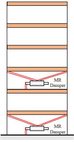
Figure 10: Six floor structure with two MR dampers. Abbreviation: MR = magnetorheological. Please click here to view a larger version of this figure.
3.1 Influence analysis of time delay
To analyze the influence of time delay on the control effectiveness of the MR damper in the MDOF structure, Figure 11 shows the maximum RMS of displacement (inter-story displacement), velocity(inter-story velocity), and acceleration (story acceleration) along with time delay for the TDC-SAC-PSO method. The parameters were  ,
, , and
, and  for the MR damper on the 1st floor;
  and
and  for the MR damper on the 3rd floor, which are the optimized results without time delay. The maximum RMS of the controlled structure responses exhibited period fluctuation along with time delay. The maximum RMS of displacement and velocity were in the 1st floor, the maximum acceleration in the 6th floor. Besides, all the maximum MRS of responses with any time delay were larger than the values without time delay, which means that time delay decreases the control effect of MR damper.
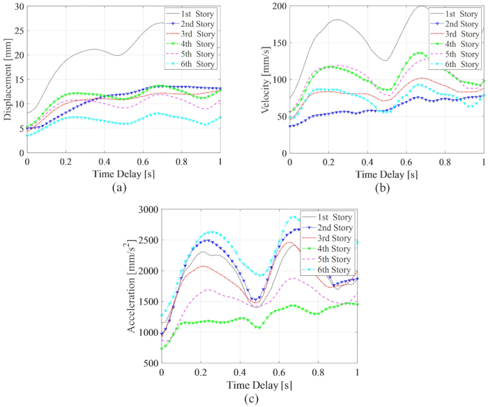
Figure 11: Maximum RMS of responses along with time delay for the TDC-SAC-PSO method-controlled structure. (A) Displacement; (B) Velocity; (C) Acceleration. Abbreviations: RMS = root-mean-square; TDC-SAC-PSO = time delayed system with compensation controlled. Please click here to view a larger version of this figure.
The reliability of displacement, velocity, and acceleration along with time delay is shown in Figure 12. The reliability of velocity and acceleration show period fluctuation along with time delay, while the reliability of displacement dramatically decreased along with time delay; all the reliability values at any time delay were less than those without time delay. Therefore, the time delay compensation method is necessary to reduce the influence of time delay on the reliability of the MR damper-controlled structure.
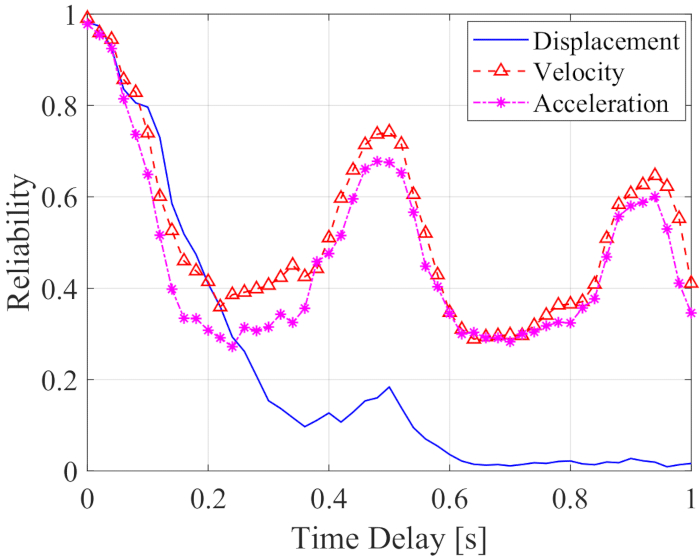
Figure 12: Reliability of controlled structure responses along with time delay. Please click here to view a larger version of this figure.
3.2 Control effect of time delay compensation
Based on the proposed TDC-SAC-PSO method, the 6-DOF structure with two MR dampers was analyzed. Figure 13 shows the RMS time histories of displacement and acceleration at the 1st and 3rd floors for the Uncontrolled (Unc), TDC-SAC-PSO method-controlled, and TDN-SAC-PSO method-controlled structures. The time delay was  , and the weighting matrix ratio ; the MR damper parameters were , for the 1st floor; and for the 3rd floor.
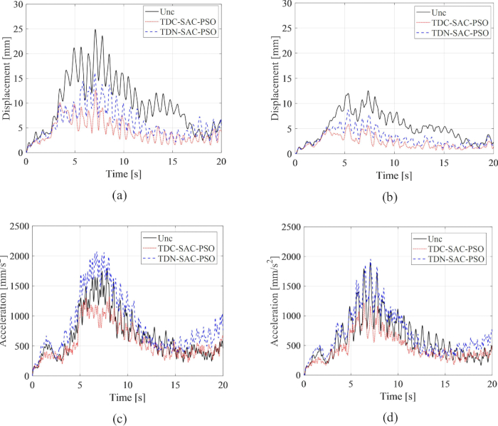
Figure 13: RMS time histories of displacement and acceleration at 1st and 3rd floors for structures controlled by different methods. (A) Displacement at 1st floor; (B) Displacement at 3rd floor; (C) Acceleration at 1st floor; (D) Acceleration at 3rd floor. Abbreviations: RMS = root-mean-square; Unc = uncontrolled; TDC-SAC-PSO = time delayed system with compensation controlled; TDN -SAC-PSO = time delayed system with non-compensation controlled. Please click here to view a larger version of this figure.
The maximum RMS of displacement at the 1st and 3rd floors were reduced 35.42% and 30.44% by the TDN-SAC-PSO method, where the time delay was not compensated. While with compensation, the maximum RMS of displacement at the 1st and 3rd floors were reduced 49.33% and 53.39%, respectively. Without compensation, the maximum RMS of acceleration at the 1st and 3rd floors increased 16.22% and 2.88% but decreased by 25.77% and 36.00%, respectively, with compensation. Therefore, the compensation of time delay in the MR damper control method is necessary for reducing the responses of structure, especially for the acceleration.
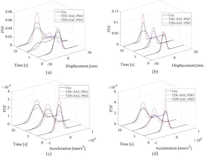
Figure 14: PDFs of displacement and acceleration at 1st and 3rd floors for different control methods. (A) Displacement at 1st floor; (B) Displacement at 3rd floor; (C) Acceleration at 1st floor; (D) Acceleration at 3rd floor. Abbreviations: PDFs = probability density functions; Unc = uncontrolled; TDC-SAC-PSO = time delayed system with compensation controlled; TDN -SAC-PSO = time delayed system with non-compensation controlled. Please click here to view a larger version of this figure.
The PDFs of displacement and acceleration at the 1st and 3rd floors are shown in Figure 14, revealing the different control effects of the TDC-SAC-PSO and TDN-SAC-PSO methods compared to the uncontrolled structure. Without compensation, the PDFs of displacement at the 1st and 3rd floors were still narrower than those of the uncontrolled structure. Further, with compensation of time delay, the PDFs of displacement became narrower than those of the TDN-SAC-PSO method-controlled structure. Unlike displacement, without compensation, the PDFs of acceleration at the 1st floor for the TDN-SAC-PSO method were wider than those of the uncontrolled structure. However, with compensation, the PDFs of acceleration at both the 1st and 3rd floors were narrower than those of the uncontrolled structure. Thus, the necessity of time delay compensation is verified for increasing the certainty of structure responses, especially for the acceleration.
| Control method | Displacement | Velocity | Acceleration | Control force at 1st floor | Control force at 3rd floor |
| Unc | 0.0114 | 0.5822 | 0.6372 | -- | -- |
| TDN-SAC-PSO | 0.5851 | 0.5258 | 0.398 | 1 | 1 |
| TDC-SAC-PSO | 0.806 | 0.8674 | 0.8037 | 1 | 1 |
Table 4: Reliability for structures controlled by different methods. Abbreviations: Unc = uncontrolled; TDC-SAC-PSO = time delayed system with compensation controlled; TDN -SAC-PSO = time delayed system with non-compensation controlled.
The reliability values of displacement, velocity, acceleration, and control force with the structure systems controlled by the different methods are shown in Table 4. The reliability values of the structure responses were calculated using the equivalent extreme value method25. By the TDN-SAC-PSO method control, the reliability of displacement increased compared with the uncontrolled structure, while the reliability of velocity and acceleration decreased. With time delay compensation in the TDC-SAC-PSO method, the reliability of displacement, velocity, and acceleration significantly increased. Besides, the reliability values of the control force for both the TDN-SAC-PSO and TDN-SAC-PSO methods are sufficiently maintained. Thus, the proposed time delay compensation control method achieves favorable control effect for the MR damper-controlled structure.
3.3 Parameter optimization
To achieve the optimal control effect, the parameters of the proposed control method were optimized based on the reliability criterion. With the time delay , the optimal result was  ;
;  , and
, and  for the 1st floor MR damper;
  and
and  for the 3rd MR damper.
The RMS time histories of displacement and acceleration at the 1st and 3rd floors are shown in Figure 15 where the control effects of the TDC-SAC-PSO and SOSC-PSO methods and the Uncontrolled structure are compared. With MR damper control, with or without time delay compensation, the RMS of displacement and acceleration decreased significantly. With the SOSC-PSO method, the maximum RMS of displacement at the 1st and 3rd floors decreased by 65.15% and 63.16% relative to the uncontrolled structure, respectively. Compared with the TDC-SAC-PSO method, the displacement response was further reduced. The maximum RMS of acceleration at the 1st and 3rd floors are decreased by 23.39% and 35.60% for the SOSC-PSO method. There was little difference in the control effect of acceleration for the SOSC-PSO and TDC-SAC-PSO methods, indicating that the control effect of time delay compensation was different for displacement and acceleration.
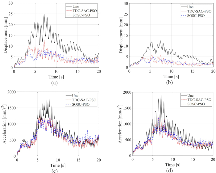
Figure 15: RMS time histories of displacement and acceleration at 1st and 3rd floors for different control methods. (A) Displacement at 1st floor; (B) Displacement at 3rd floor; (C) Acceleration at 1st floor; (D) Acceleration at 3rd floor. Abbreviations: RMS = root-mean-square; Unc = uncontrolled; TDC-SAC-PSO = time delayed system with compensation controlled; SOSC-PSO = Stochastic Optimal Semi-active Control method with time delay compensation. Please click here to view a larger version of this figure.
The PDFs of displacement and acceleration at the 1st and 3rd floors are presented in Figure 16; the PDFs of displacement and acceleration were narrowed by the TDC-SAC-PSO and SOSC-PSO methods compared with the Uncontrolled structure. Besides, the PDFs of displacement and acceleration for the SOSC-PSO method were further narrowed compared to those of the TDC-SAC-PSO method-controlled structure. Therefore, with parameter optimization, the proposed time delay compensation control method achieved a better control effect than without optimization.
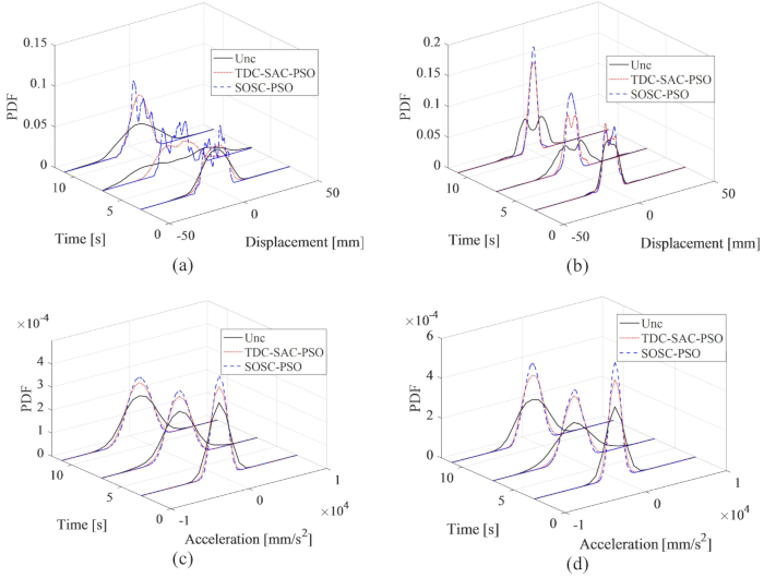
Figure 16: PDFs of displacement and acceleration at 1st and 3rd floors for different control methods. (A) Displacement at 1st floor; (B) Displacement at 3rd floor; (C) Acceleration at 1st floor; (D) Acceleration at 3rd floor. Abbreviations: PDFs = probability density functions; Unc = uncontrolled; TDC-SAC-PSO = time delayed system with compensation controlled; SOSC-PSO = Stochastic Optimal Semi-active Control method with time delay compensation Please click here to view a larger version of this figure.
The reliability values of displacement, velocity, acceleration, and control force are shown in Table 5. The reliability values for the SOSC-PSO method were higher than those for the TDC-SAC-PSO method. Meanwhile, the control force still retained sufficient reliability. Thus, the optimization of parameters is necessary for achieving the best control effect for the MR damper-based control method.
| Control method | Displacement | Velocity | Acceleration | Control force at 1st floor | Control force at 3rd floor |
| Unc | 0.0114 | 0.5822 | 0.6372 | -- | -- |
| TDC-SAC-PSO | 0.806 | 0.8674 | 0.8037 | 1 | 1 |
| SOSC-PSO | 0.9544 | 0.9314 | 0.8788 | 1 | 1 |
Table 5: Reliability for structures controlled by different methods. Abbreviations: Unc = uncontrolled; TDC-SAC-PSO = time delayed system with compensation controlled; SOSC-PSO = Stochastic Optimal Semi-active Control method with time delay compensation.
Access restricted. Please log in or start a trial to view this content.
Results
Aiming at the influence of time delay on the control effectiveness of the MR damper-based method, a semi-active control method with time delay compensation is proposed in this paper. In the proposed method, the critical parameters are optimized based on the reliability criterion. By comparing the control effectiveness, the following conclusions are addressed:
(1) The semi-active control method based on an MR damper is more robust than the active control method. Even with time delay, semi-activ...
Access restricted. Please log in or start a trial to view this content.
Discussion
With the introduction of the Physical Stochastic Optimal control theory (PSO), a Stochastic Optimal Semi-active Control method with time delay compensation (SOSC-PSO) is proposed in this paper, which is designed to maintain the reliability of structures controlled by MR dampers. To compensate for the time delay in the proposed method, the semi-active control force is derived as the function of not only the present states but also the states and control forces in previous time steps in discrete state space. To achieve the...
Access restricted. Please log in or start a trial to view this content.
Disclosures
All authors have no conflicts of interest to declare.
Acknowledgements
The authors gratefully acknowledge the support of the Natural Science Foundation of Hebei Province (Grant No. E2023210007).
Access restricted. Please log in or start a trial to view this content.
Materials
| Name | Company | Catalog Number | Comments |
|---|---|---|---|
| MATLAB | MathWorks | 2016 | Using for the calculation of the proposed method |
References
- Yao, J. T. P. Concept of structural control. J Struct Div. 98 (7), 1567-1574 (1972).
- Liu, J., Silva, C. E., Dyke, S. J., Wu, Y., Liu, H. Using real-time hybrid simulation for active mass damper experimentation and validation. Mech Mach Theory. 191, 105474(2024).
- Pan, H., Li, C., Cao, L. Bidirectional pendulum-type tuned tendem mass dampers-inerters for integrated control of alongwind and crosswind responses in super-tall buildings. J Build Eng. 100, 111676(2025).
- Housner, G. W., et al. Structural control: past, present, and future. J Eng Mech. 123 (9), 897-971 (1997).
- Rahman, M., Ong, Z. C., Chong, W. T., Julai, S. Smart Semi-active PID-ACO control strategy for tower vibration reduction in Wind Turbines with MR damper. Earthq Eng Eng Vib. 18 (4), 887-902 (2019).
- Morales-Beltran, M., Paul, J. Active and semi-active strategies to control building structures under large earthquake motion. J Earthquake Eng. 19 (7), 1086-1111 (2015).
- Shu, Z., You, R., Xie, Y. Viscoelastic dampers for vibration control of building structures: A state-of-art review. J Earthq Eng. 28 (12), 3558-3585 (2024).
- Soong, T. T. Active structural control: Theory and practice. Longman Scientific & Technical. , New York. (1990).
- Wan, H. P., Ma, Q., Dong, G. S., Luo, Y., Ni, Y. Q. Data-driven model reduction approach for active vibration control of cable-strut structures. Eng Struct. 302, 117434(2024).
- Cao, L., Li, X., Huang, Y., Li, C., Pan, H. High robust eddy current tuned tandem mass dampers-inerters for structures under the ground acceleration. Soil Dyn Earthq Eng. 188, 109040(2025).
- Chha, H., Peng, Y. Adaptive semiactive control of structure with magnetorheological dampers using wavelet packet transform. Adv Struct Eng. 27 (9), 1509-1527 (2024).
- Zeng, X., Peng, Y., Chen, J. Serviceability-based damping optimization of randomly wind-excited high-rise buildings. Struct Des Tall Spec. 26 (11), e1371(2017).
- Li, C., Chang, K., Cao, L., Huang, Y. Performance of a nonlinear hybrid base isolation system under the ground motions. Soil Dyn Earthq Eng. 143, 106589(2021).
- Cao, L., Li, C. A high performance hybrid passive base-isolated system. Struct Control Health Monitoring. 29 (3), e2887(2022).
- Zareie, S., Issa, A. S., Seethaler, R., Zabihollah, A., Ahmad, R. A novel SMA-magnetorheological hybrid bracing system for seismic control. Eng Struct. 244, 112709(2021).
- Chu, S. Y., Soong, T. T., Reinhorn, A. M. Active, hybrid and semi-active structural control. , John Wiley & Sons. New York. (2005).
- Danielian, S. A., Jabbari, F., Zareian, F. Effects and distribution of semi-active resettable springs on the seismic response of asymmetric structures. Earthq Eng Struct D. 52 (10), 2966-2982 (2023).
- Shuang, Z., Wenliuhan, H. S., Liu, Y. H., Inoue, N., Zhai, Z. P. Seismic response control for bridge piers with semi-active MR damper based on displacement feedback. J Earthq Eng. 28 (3), 849-865 (2024).
- Wang, Y., Dyke, S. Modal-based LQG for smart base isolation system design in seismic response control. Struct Control Health Monitoring. 20 (5), 753-768 (2013).
- Desai, R. M., et al. Performance evaluation of a single sensor control scheme using a twin-tube MR damper based semi-active suspension. J Vib Eng Technol. 9, 1193-1210 (2021).
- Abdi, M. S., Nekooei, M., Jafari, M. A. Seismic control of multi-degrees-of-freedom structures by vertical mass isolation method using MR dampers. Earthq Eng Eng Vib. 23 (2), 503-510 (2024).
- Bhowmik, K., Debnath, N. Semi-active vibration control of soft-storey building with magnetorheological damper under seismic excitation. J Vib Eng Technol. 12 (4), 6943-6961 (2024).
- Yang, J. N., Akbarpour, A., Askar, G. Effect of time delay on control of seismic-excited buildings. J Struct Eng. 116 (10), 2801-2814 (1990).
- Temimi, H., Ben-Romdhane, M., El-Borgi, S., Cha, Y. Time-delay effects on controlled seismically excited linear and nonlinear structures. Int J Struct Stab Dyn. 16 (7), 1550031(2016).
- Peng, J., Wang, L., Zhao, Y., Lenci, S. Time-delay dynamics of the MR damper-cable system with one-to-one internal resonances. Nonlinear Dynamics. 105 (2), 1343-1356 (2021).
- Cha, Y. J., Agrawal, A. K., Dyke, S. J. Time delay effects on large-scale MR damper based semi-active control strategies. Smart Mater Struct. 22 (1), 015011(2013).
- Yu, Y., et al. Experimental study of wireless structural vibration control considering different time delays. Smart Mater Struct. 24, 045005(2015).
- Ahmadizadeh, M., Mosqueda, G., Reinhorn, A. M. Compensation of actuator delay and dynamics for real-time hybrid structural simulation. Earthq Eng Struct Dyn. 37 (1), 21-42 (2008).
- Bathaei, A., Zahrai, S. M. Compensating time delay in semi-active control of a SDOF structure with MR damper using predictive control. Struc Eng Mech. 82 (4), 445-458 (2022).
- Dyke, S. J., Spencer, B. F. Jr, Sain, M. K., Carlson, J. D. Modeling and control of magnetorheological dampers for seismic response reduction. Smart Mater Struct. 5 (5), 565-575 (1996).
- Ying, Z. G., Ni, Y. Q., Ko, J. M. A semi-active stochastic optimal control strategy for nonlinear structural systems with MR dampers. Smart Struct Syst. 5 (1), 69-79 (2009).
- Rosol, M., Martynowicz, P. Implementation of the LQG controller for a wind turbine tower-nacelle model with a MR tuned vibration absorber. J Theor App Mech-Pol. 54 (4), 1109-1123 (2016).
- Lyu, M. Z., Feng, D. C., Chen, J. B., Li, J. A decoupled approach for determination of the joint probability density function of a high-dimensional nonlinear stochastic dynamical system via the probability density evolution method. Comput Method Appl M. 418 (A), 116443(2024).
- Chha, H., Peng, Y. Multiscale stochastic optimal control of hysteretic structures based on wavelet transform and probability density evolution method. Eng Computation. 41 (4), 865-896 (2024).
- Li, J., Peng, Y. B., Chen, J. B. A physical approach to structural stochastic optimal controls. Probabilist Eng Mech. 25 (1), 127-141 (2010).
- Peng, Y. B., Yang, J. G., Li, J. Seismic risk-based stochastic optimal control of structures using magnetorheological dampers. Nat Hazards Rev. 18 (1), B4016001(2017).
- Dong, X. M., Yu, M., Li, Z., Liao, C., Chen, W. Neural network compensation of semi-active Control for magneto-rheological suspension with time delay uncertainty. Smart Mater Struct. 18 (1), 015014(2008).
- Peng, Y. B., Zhang, Z. Optimal MR damper-based semiactive control scheme for strengthening seismic capacity and structural reliability. J Eng Mech. 146 (6), 04020045(2020).
- Luo, M. X., Gao, M., Cai, G. Delayed full-state feedback control of airfoil flutter using sliding mode control method. J Fluid Struct. 61, 262-273 (2016).
- Xu, J., Chung, K. W., Chan, C. L. An efficient method for studying weak resonant double Hopf bifurcation in nonlinear systems with delayed feedbacks. Siam J Appl Dyn Syst. 6 (1), 29-60 (2007).
- Yang, J. S., Jensen, H., Chen, J. B. Structural optimization under dynamic reliability constraints utilizing probability density evolution method and metamodels in augmented input space. Struct Multidiscip Optimization. 65, 107(2022).
- Li, J., Chen, J. B. Stochastic dynamics of structures. , John Wiley & Sons. Singapore. (2009).
- Peng, Y. B., Li, J. Stochastic optimal control of structures. , Springer. (2019).
- Dowrick, C. Beyond depression: A new approach to understanding and management. , Oxford University Press. (2009).
- Wang, D., Li, J. Physical random function model of ground motions for engineering purposes. Sci China Technol Sci. 54 (1), 175-182 (2011).
- Wang, D., Li, J. A random physical model of seismic ground motion field on local engineering site. Sci China Technol Sci. 55 (7), 2057-2065 (2012).
- Chen, J. B., Li, J. Strategy for selecting representative points via tangent spheres in the probability density evolution method. Int J Numer Meth Eng. 74 (13), 1988-2014 (2008).
Access restricted. Please log in or start a trial to view this content.
Reprints and Permissions
This article has been published
Video Coming Soon