High-throughput Serial Tomography using an Automated Sample-changing Robot

Summary

The implementation details and data collection procedure for synchrotron-based X-ray tomography using the automated sample-changing robot at Diamond Light Source (DLS) I13-2 Imaging beamline are presented and discussed here. This improves the throughput and the data collection efficiency of the beamline drastically.

Abstract

This manuscript describes a workflow for automated data collection that uses a robotic arm for sample exchange, significantly improving data collection efficiency. The setup, implemented for synchrotron X-ray imaging at the Diamond Light Source (DLS) I13-2, Imaging beamline, utilizes a robot to achieve high-throughput serial tomography (3D) or imaging (2D). At present, for many experiments, the time required for manual sample exchange and alignment is comparable to, or even exceeds, the duration of the tomography scan itself. To maximize the efficient use of available beam time and increase experimental throughput, automating sample exchange and alignment is essential. Using the robot as a sample changer can increase throughput by at least 4-10 times compared to manual procedures, depending on which pixel size is chosen. With the Diamond II machine and the I13L beamlines Operando Coherent TOmography and Ptychographic Imaging (OCTOPI) upgrades, the increased X-ray flux will further reduce the experimental scan times, making the system even more efficient. Furthermore, the automation enables remote data collection, including an optional mail-in service for users. Automated sample centering allows fully unattended scanning, which can be performed remotely. This represents a unique and innovative feature of the system. This manuscript describes the complete procedure, including sample preparation, mounting on specialized holders, transport to the beamline, and placement on the dedicated trays for robotic sample exchange. The procedure for automated sample centering and the subsequent tomography reconstruction pipeline are  presented.

Introduction

Automation has been widely used in the heavy manufacturing industries for decades^1,2,3. However, robotic hardware and software development has matured sufficiently so that it can handle very delicate jobs such as genome sequencing, conducting medical surgeries in hospitals, or assisting in running chemistry experiments^4,5,6,7. Automation not only eliminates human errors but also improves throughput and efficiency⁴.

A synchrotron X-ray source generates extremely bright and highly coherent electromagnetic radiation in the broad spectral range from infrared to hard X-rays. These sources enable high-throughput and high-resolution imaging experiments with very short scan times and high statistics. The partial coherence can be utilized to achieve better contrast for weakly absorbing soft materials such as polymers or tissue samples^8,9,10 in comparison to laboratory-based X-ray sources. A full X-ray tomography data set – which allows for the visualization of an object in real 3D – requires the acquisition of projections of the sample at different angles. Advances in source brightness, experimental hardware, and controls allow for data collection times in the range of tens of seconds to minutes⁸. As a result, sample loading and alignment have become more time-consuming than the tomography scan itself^11,12. It is important to note that changing samples manually in a synchrotron tomography experiment can take a significant amount of time (compared to scan time), since a radiation safety procedure needs to be followed while entering and closing the experimental hutch. This procedure takes several minutes, typically. In addition, sample alignment can also take up a few minutes.

If this process of sample changing and sample alignment is automated, a significant amount of time will be saved. Therefore, a sample changer robot has been implemented at the I13-2 Imaging beamline of the DLS synchrotron facility. This manuscript describes the full protocol of performing a synchrotron X-ray micro-tomography experiment with multiple samples using a sample changer robot at the I13-2 Imaging beamline^11,12. This implementation not only improves the efficiency of the experimental time but also allows experiments to be conducted remotely. The alternative is manual or semi‑automated operation, both of which are significantly slower. Here, semi-automated means using the robot for sample exchange only without sample alignment.

The significance of automation is underlined by automation projects at other synchrotron imaging beamlines, with the most similar projects at the 2BM beamline of APS¹³, the SLS TOMCAT beamline¹⁴, the EMBL P14 beamline on PETRA III¹⁵, and the IMAGE beamline at the Karlsruhe Institute of Technology (KIT) Light Source¹⁶. In the 2-BM APS, the samples requiring scanning with a robot are mounted on a standard kinematic mount, which is placed in a sample changer tray of maximum capacity of 60 samples at a time. A gripper arm then picks the sample and mounts it on the rotation stage. However, the sample alignment is done offline using a stereoscope. A similar system was installed in the TOMCAT beamline in SLS, except here the process is fully automated, which can perform sample load-unload, alignment, scanning a correct region of interest, and reconstruction. The total number of samples that can be scanned at a time is 60. Recently, the P14 beamline on PETRA III¹⁵ has installed a sample changing system which can handle soft biological samples of the order of 1 mm in size. Positioning and centering are done by the three-click-centering procedure. At the IMAGE beamline at KIT, a high‑throughput imaging/tomography end‑station enables the measurement of up to 1,500 specimens within two days¹⁶. Different from the robot systems mentioned above, the I13‑2 Imaging beamline system can currently handle samples up to 8 mm in diameter and measure up to 112 samples within an eight‑hour shift, without human intervention, including automatic sample centering.

The current tomography setup at I13-2, Diamond-Manchester Imaging beamline, has been reported in the publication mentioned¹⁷. For completeness, key aspects of the tomography experiments are summarized here; please also refer to Figure 1. The tomography stage stack consists of a hexapod (PI miCos) for sample manipulation as well as rotation axis tilt alignment. An air-bearing rotation stage is mounted on top of the hexapod. The rotation stage has excellent wobble (<2.4 µrad) and axial error (<100 nm) motions. The tomography detector system is equipped with four different magnifications (or field of view). For the current study, 1.25× (2.6 µm effective pixel size with 6.7 mm x 5.6 mm field of view) and 4× (0.81 µm effective pixel size with 2.1 mm x 1.8 mm field of view) objectives have been used. The 1.25× objective had a 500 µm LuAg:Ce scintillator, whereas the 4x objective had a 100 µm LuAg:Ce scintillator (Crytur). A sCMOS detector (pco.edge 5.5) records the magnified scintillation screen image via an additional 2x photo eyepiece (all microscope optics are from Olympus). The effective pixels range from 2.6 µm to 0.33 µm, with about 1 µm resolution at the highest magnification used. The detector chip consists of 2560 x 2160 with 6.5 µm pixel size, and the maximum readout rate of the pixel array is 100 Hz.

Protocol

NOTE: This study uses insect specimens from the Natural History Museum (NHM), London, for comparative phenotypic analysis. Specimens had been acquired by the Natural History Museum, following standard acquisition procedures to ensure that specimens had been legally collected and donated.

1. Planning of the experiment

1. Check the feasibility of performing tomography or imaging experiments with the sample of interest at the I13-2 beamline by contacting the beamline staff using the following link: https://www.diamond.ac.uk/Instruments/Imaging-and-Microscopy/I13-2/Staff.html .
2. Submit a proposal to obtain a timeslot for performing the planned experiment using the following link: https://www.diamond.ac.uk/Users.html.
3. Discuss sample preparation and the sample measurement process with beamline staff once the proposal is accepted and the experiment is scheduled. Experiments conducted using the robot have certain requirements, which are provided in the next section (section 2).
4. Discuss the sample dimensions and composition with the beamline staff to verify that the experiment can be performed successfully at the beamline.
5. Start preparing for the experimental visit well in advance by following the instructions on the website (https://www.diamond.ac.uk/Users.html).
6. Complete the safety training before the experimental session.

2. Sample preparation (for robot experiments)

1. Prepare SPINE-Compatible Sample Bases¹⁸ for sample mounting. Mount each sample on a SPINE‑style standard sample base equipped with a Data Matrix barcode to enable automated sample tracking.
2. Attach the sample to the base using one of two configurations. Pin mounting: Fix the sample on a SPINE‑style sample pin (see Figure 1C, inset). Container or direct mounting: Place the sample inside a compatible container, such as a micro‑centrifuge tube/polyimide tube, or directly on the sample base.
3. Check dimensional compatibility with the robot gripper by verifying that the mounted sample falls within the allowed size envelopes to ensure safe robotic handling (see Figure 2):
   Option A: Fits inside an 8 mm diameter x 20 mm height cylinder.
   Option B: Fits inside a 3.5 mm diameter x 33 mm height cylinder.
4. Ensure that both configurations are centred on the sample base. Make sure that the total height (sample + mount + base) does not exceed 27 mm or 40 mm, depending on the chosen configuration.
5. When mounting samples on SPINE sample pins, ensure that the sample is positioned on top of the pin, with no part of it obscured by the pin shaft. The sample must be mounted vertically and centrally on the pin base to prevent contact with the robot gripper. This is particularly important for the Option B mounting described in protocol section 2.3, as well as for elongated samples that are mounted on top of the sample pins.
6. When mounting inside containers or tubes, secure the sample firmly inside the container so that it does not shift during transport or robotic handling. Make sure the container itself remains vertically aligned on the sample base.
7. Fix the chosen mounting element (pin or container) securely and vertically onto the sample base to ensure positional stability throughout the experiment.
8. Use a reliable adhesive or securing method to prevent detachment during shipping and automated manipulation, as both processes may introduce mechanical stresses.
   NOTE: Common adhesives include cyanoacrylate (super glue), paraffin wax, and hot‑melt glue. Consult beamline staff if uncertain about material compatibility.
9. Check that all samples are positioned at a consistent height from the container’s top edge or on the sample pin. For samples mounted inside containers, make sure that the lateral distance from the container wall is the same across all the samples.
   NOTE: Consistent positioning is essential for reliable automatic alignment. Smaller samples relative to the field of view allow more tolerance.
10. Document the Data Matrix code associated with each sample to ensure correct sample identification during data analysis.
11. Generate a samples.csv file to relate each sample name to its sample base data matrix code and to pass on the parameters relevant for running tomography scans.

3. Sample packaging and delivery

1. No later than 15 working days before the experimental session, submit the experimental risk assessment (ERA) and declare all samples there. This ERA needs to be approved by the DLS health and safety (HSE) group before samples are allowed to be shipped/brought on site.
2. Use the universal sample base with the sample pin-mounted combination storage and/or shipping container, also called Uni-puck. This is rather important if sending by post.
3. If samples do not fit within the sample slots of the storage container mentioned in step 3.2, please make alternate mounting arrangements, such as using magnetic protective caps that fit the sample base and directly bring the samples for measurements.

4. Experimental setup

1. Adjust the X-ray source parameters to maximize contrast in the sample. To achieve this, shift the full spectrum and/or filter the X-ray spectrum.
2. Optimize the camera to sample distance based on the X-ray spectrum and the degree of phase contrast desired for a given sample.
3. Select the microscope magnification based on the sample size and required field of view, and select the corresponding microscope objective.
4. Align the camera horizontal position (x-axis in the lab) with respect to the X-ray beam.

5. Sample loading and alignment

1. Check samples and sample mounting thoroughly at the start of each experimental session for any samples that appear to be damaged or loosely mounted. Inform users about any such samples.
   NOTE: At present, the beamline is equipped with mounts for up to 7 pucks, and each puck can hold up to 16 samples. A total of 112 samples can be measured during a single robot run. Please refer to Supplementary Figure 2, which illustrates how to identify the puck slot (pin) positions.
2. Mount samples on the respective puck and puck-slots (pins) as identified in the samples.csv file. Perform a dry run of the robot sample exchange procedure on a few samples to test the working of the robot, as well as to make sure samples are within the required specification.
3. Use a sample base with a sample pin (without a sample) for aligning the axis of rotation of the rotation stage to the center of the detector in the horizontal direction.
4. Move the top of the pin to the center of the X-ray camera (Figure 3A). Align the telescope camera (TC), which is set up at 90° to the beam, as shown in the picture (Figure 3), to be in the center of the field of view (FOV). Determine the co-ordinates of this position in TC pixel coordinates.
5. Update the sample target position in the script that handles the sample alignment.
6. Mount a representative sample. Run the automatic sample alignment script to place the sample in the center of rotation on the TC. The link to the script is provided in Supplementary File 1.
7. Check if the sample region of interest (ROI) is centered in the field of view (FOV) of the X-ray camera.
8. If the ROI is not centered in the FOV, repeat steps 5.5 to 5.7 and refine the sample alignment by changing the coordinates for the target position.
   NOTE: Sections 4 and 5 are performed by the local contact except section 4.2.

6. Data acquisition setup

1. Check that the required file/folder structure on the DLS file system has been created to store raw data, metadata files, and analysis results.
2. Copy the samples.csv file to the folder mentioned in step 6.1.
3. Update the camera exposure time and number of projections to acquire in the samples.csv, based on the sample structure and desired contrast.
4. Define two groups of motor positions called Loading Position (LP) and Scanning Position (SP). LP is the set where stages are optimized for sample loading, and the SP for tomography scanning of the sample.
   NOTE: Section 6 is performed by the local contact or automatically created by the DLS systems.

7. Performing data collection

1. Mount all samples on the correct puck and pin positions, as instructed in the samples.csv file.
2. For the data collection, use the Generic Data Acquisition (GDA) workbench, an open-source software developed by DLS ( https://alfred.diamond.ac.uk/documentation/manuals/GDA_User_Guide/master/introduction.html). It is a Java-based system used in DLS to control experiments and collect data. A screenshot is provided in Supplementary Figure 1.
3. Use an object called tomomatic in GDA for automatic sample changing, sample alignment, and tomography measurement.
4. Issue the command tomomatic.load (/dls/i13/data/year/… samples.csv) in the GDA terminal to load the file. Then issue the tomomatic. scan () for running the command.
5. The robot first picks up the sample from the loading tray and takes it to the laser barcode reader. Once the barcode has been read, it moves the sample to the tomography stage and mounts it. Ensure that the entire process runs smoothly.
   NOTE: Here, a Yaskawa robot with the in‑house‑developed flexure gripper is being used.
6. Once sample loading is performed, the stages move to the SP position. Then, autoCentrePin function within the tomomatic script is executed, which places the sample into the Center of Rotation (COR). The X-ray tomography measurement with a robot sample changer is now ready to be performed.
   NOTE: Please check the Supplementary File 1 for the pseudo code of the tomomatic script.
7. Carry out the execution of the TomoFlyscan function for the tomography measurement. The function first collects 40 projection images without X-ray beam, referred to as a dark image (DI), and 40 images with X-ray beam but without a sample in the beam, referred to as a flat-field image (FI). These images will be used for image normalization during data reconstruction.
8. Collect Projection images (PI) with the sample in the beam at sample rotation angle intervals, as indicated in the samples.csv file. For the present case, it has 3001 PI images.
   NOTE: All of the steps, from 7.5 to 7.8, proceed one after the other without any human intervention.

8. Accessing the data and analysis

1. Access the saved data by browsing to the appropriate file system and folder. The scanned data mentioned in the previous section is saved in two different files, one with *.nxs and *.hdf file with * being a numerical number, for example: 123456.nxs and 123456.hdf. The NXS contains the metadata for the scan, whereas the HDF contains all the projection image data (linked data from NXS).
2. Use Savu reconstruction pipeline¹⁹ for generating 2D slices from projection images.
3. Access and visualize the reconstructed images using 3D rendering software, such as AVIZO/ ImageJ.
   NOTE: Completion of sections 7 and 8 requires coordinated actions from both users and local contacts, with individual sub‑steps performed by each.

Results

Figure 1 shows the Yaskawa GP7 sample-changer robot installed on the Diamond I13-2 Imaging beamline. Figure 1A shows the robot (1) and the in-house designed flexure gripper (2). This gripper can hold a sample with a diameter of ≤ 8mm. Figure 1B shows the robot (1) and optics/X-ray camera system (4) and (6) used for acquiring tomography data. The robot gripper picks the sample from the sample tray (3), which can hold 7 uni-pucks with 16 samples on each, as shown in Figure 1C. Samples are mounted on the aluminum dowel (5), and the tomography data acquisition is performed with the detector system (6). The details of (5) and (6) are provided in the last paragraph of the introduction section. The red broken line in Figure 1B indicates the X-ray beam direction.

Details of the sample mounting scheme and the flexure gripper design are illustrated in Figure 2. Figure 2A shows a cylindrical plastic sample, fabricated by 3D printing, glued to the sample base. The boundary of the sample represents the envelope of the maximum sample height and the diameter. The red arrows indicate the position where the flexure gripper holds the sample base to move it from the sample tray to the tomography stage and vice versa. A 3D design of the flexure gripper is shown in Figure 2B. Fingers of the gripper are actuated by a pneumatically controlled drive tube (Figure 1B, item 2). The central space in the gripper has a diameter of 8.9 mm, as shown in Figure 2C, allowing a maximum sample size of 8 mm with a margin of ~1 mm. Figure 2D shows the picture of the top of the tomography stage. An Aluminum dowel is mounted on top of the two orthogonal stages and a magnetic disc, which has an exact diameter such that the recess on the bottom of the sample base fits. Since this disc is magnetic, it holds the mounted sample base firmly in place during the tomography measurements.

For this representative experiment, 64 insect samples provided by the Natural History Museum (NHM) in London have been selected. Specimens were selected to represent a range of arthropod phenotypes while fitting within the size constraints of the gripper. As arthropods, particularly insects, represent the vast majority of known species diversity, with over 1 million named species, they are particularly challenging to sample for comparative studies of phenotype. The present sample therefore demonstrates the potential of this approach by sampling three class-level clades of arthropods: Arachnida, Entognatha, and Insecta, as well as sampling more finely within insects to capture variation in seven orders, including four of the most species-rich orders alive today. Specimens were fixed to a card with adhesive. The cards were then mounted on the sample pins. Mounting samples (insects) directly on the sample pins is avoided since a highly absorbing structure in the beam with low absorption samples will create streak artifacts during the reconstructions, besides the difficulty of mounting them securely on sample pins. Table 1 shows the template samples.csv file that the user will fill in with the required parameters for the tomography (columns A, B, C, E, F, G, H, K). The description of each of the columns is provided in the table. The columns D, I, J, and L in the input_file are filled in after alignment and optimization of the tomography parameters at the beamline. All 64 samples were first measured with a 1.25x objective (FOV of 6.7 mm x 5.6 mm) at an optimized X-ray propagation distance (from sample to detector), and later the same samples were measured with a 4x objective using its own optimized parameters. Once the samples are loaded onto the sample tray and the experimental hutch is secured, the scan is initiated with GDA.

Automatic alignment of the sample was performed by a script written in Python (Location of the file on GitHub: https://gist.github.com/ndg63276/9b3c5cfe7db26b14930dff3ef889e2bc). At first, sample alignment is set up using a sample base and a sample pin combination without the sample. Figure 3 shows the sample pin, as seen by the side telescope camera (camera positioned at 90° to the X-ray beam- Figure 1B, item 4), which is used as a standard alignment sample. The telescope camera image is binarized so that the sample can be detected from the background. Edges of the sample are determined and marked as a white boundary, as shown in Figure 3. The reference coordinate position of the sample is the top of the pin marked as a white circle in the inset of Figure 3A. Looking at the X-ray image, the ROI of the sample is positioned on the COR, and the required target coordinate position, marked as a blue double-headed arrow cross with a red dot (Figure 3B), is determined on the side camera. This target position setting allows placing the sample not only on the COR, but also a few mm higher/ lower or a bit off center, if needed. After the sample has been loaded on the tomography stage, the automatic centering function is executed. The script first moves the sample to the target position (Figure 3B) and goes to 0°. Next, it moves the sample to 90° (Figure 3C) and determines how much sample needs to be moved to put the sample into the center of rotation (COR). This usually takes about 15-20 s. The sample is now on the COR (Figure 2D), and COR has already been aligned with the center of the camera. The system is now ready for tomography acquisition.

In this NHM insect study, 128 tomography scans were performed without human intervention. The measurement took a total of 17 h. Each scan was about 8 min. Such an experiment without the use of the robot would have taken about 20 to 25 min per tomography scan. This implies that tomography scans with robots are 3-4 times faster than scanning manually for the present case. Table 2 shows a typical log file generated at the end of a robot batch scan, including the parameters required to link each scan number to its corresponding sample. Additional details are provided in the Table 2 legend.

Figure 4 shows normalized projection images of one of the samples, an insect (Class – Insecta, order – Coleoptera), imaged during the tomography experiment mentioned above with 1.25x and 4x magnification. The top row, Figure 4A-C, shows a sample imaged with 1.25x, and then the same sample was imaged with 4x, i.e., Figure 4D-F. Figure 4 A–F displays the projection images acquired at 0°, 90°, and 180°. The yellow rectangle shows the FOV of the zoomed-in projection images that are acquired with a 4x objective. It is important to note that once the samples were loaded on the tray shown in Figure 1C, all the processes proceeded without any human intervention. Please note that these two scans were acquired ~8.5 h apart. This indicates the stability and the reproducibility of the setup.

Figure 5 shows horizontal or transverse slices from the set of tomography reconstruction slices of the sample mentioned in Figure 4. Both the 1.25x (Figure 5A) and 4x (Figure 5B) slices are plotted without cropping the images and have 2510 x 2510 pixels. The slices are well-centered within the FOV, which shows that zooming into a region with higher magnification is possible without the need for any physical intervention.

The results presented here demonstrate that implementing a robotic system for sample exchange in synchrotron micro‑tomography experiments provides several significant advantages. These include increased throughput, improved operational efficiency, and the capability to conduct scans at multiple magnifications (zoom‑in) without requiring human intervention. Considering the number of samples that need to be scanned, such as in the NHM study presented here, it would be impossible to obtain statistically robust and consistent conclusions through manual scanning.

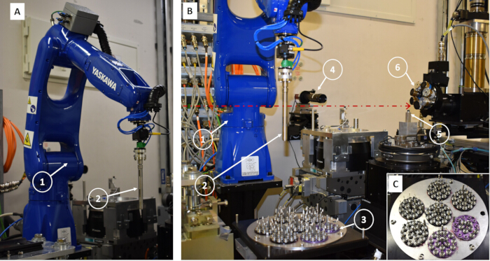
Figure 1: Picture of the robot and the tomography experimental setup installed in the I13-2 beamline. (A) The robot (1) with an in-house designed flexure gripper (2). (B) The sample loading tray (3) and the tomography stage (5). The Optical camera (Telescope camera), indicated as (4), is used for aligning the samples onto the COR. The detector system (6) used for measurement contains multiple motorized objectives for changing the field of view automatically, and a pco.edge 5.5 detector. The red dashed arrow represents the X-ray beam direction. (C) Picture of the sample loading tray with 7 pucks, and each puck can hold up to 16 samples mounted on a combination of sample base and sample pins. Please click here to view a larger version of this figure.

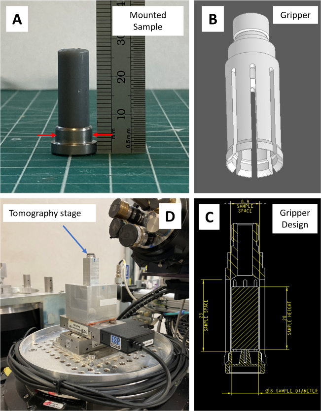
Figure 2: Details of the sample mounting scheme and the flexure gripper design. (A) Picture of a 3D-printed plastic dummy sample mounted on a sample base, representing the maximum sample envelope that can be handled by the flexure gripper. The red arrows indicate the position where the gripper holds the sample base. (B) 3D design of the flexure gripper. The fingers of the gripper are actuated to hold or release the sample base. (C) Vertical section drawing of the gripper with dimensions. The maximum opening in the center is 8.9 mm; therefore, the maximum allowable sample size is ≤ 8mm. (D) Picture of the top of the tomography stage. An Aluminum dowel (indicated by the blue arrow) is mounted at the top of the two orthogonal stages. A magnetic disc is fixed to the top of the dowel on which the sample base (with the sample) is positioned by the gripper. Please click here to view a larger version of this figure.

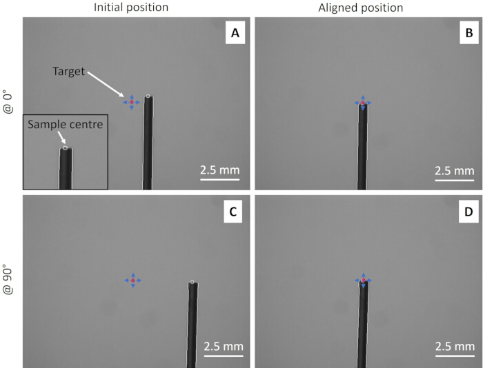
Figure 3: Snapshots from the video graph of the COR alignment procedure using the side telescope camera. (A) Picture of the alignment pin just before the alignment routine starts. Blue double-headed cross with central red dot is the target position, which coincides with the COR of the tomography rotation stage. The inset shows the zoomed image of the top of the pin showing the detected sample center, both in height and width. (B) Pin aligned to the target position at 0°. (C) Pin rotated to 90°, and it is off target position. (D) Pin aligned to the target position at 90°. Now the pin is aligned in both orthogonal directions; therefore, the sample will rotate in the center of the camera. Please click here to view a larger version of this figure.

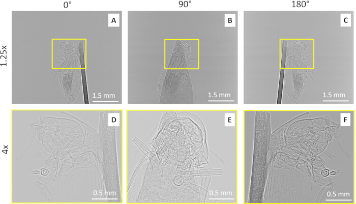
Figure 4: Normalized projection images of an insect collected with a 1.25x and a 4x objective. The insect belonged to the class Insecta, order Coleoptera. This represents two out of 128 tomography scans. The insect was glued onto a paper and attached to the sample pin. Projection images with 1.25x objective are at (A) 0°, (B) 90°, (C) 180°, and with 4x at (D) 0°, (E) 90°, and (F) 180°. The set of 1.25x and 4x tomography scans were collected in a single session without any human intervention. A set of images with 1.25x provides a full view of the sample, and a 4x set of images shows zooming capability. Please click here to view a larger version of this figure.

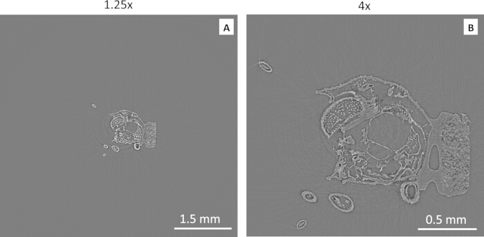
Figure 5. Comparison of an identical tomographic slice acquired using two different fields of view. A single reconstructed slice from tomography of the projection images displayed in Figure 4 for (A) 1.25x and (B) 4x magnifications. Please click here to view a larger version of this figure.

Table 1: Typical samples.csv file that the user provides containing tomography parameters. This file is read by the tomomatic Python script that is used for data acquisition. The columns A (description of the sample), B (puck ID), C (slot in the puck), E (tomography rotation step), F (number of FI), G (number of DI), H (magnification to be used), and K (slot priority) are filled in by the user. The columns D (exposure time), I (X-ray propagation distance between sample and camera), J (Camera motion across beam to place the COR to the center of the camera), and L (barcode of the sample base) are filled in after the alignment and preliminary optimization. Please click here to download this Table.

Table 2: Typical output log file saved as Output_file.txt after all the samples have been scanned. The file reports all the input parameters, and in addition, it provides the barcode of the sample scanned (column M), path to the scanned metadata and image files (column N), and the position of the motor used for collecting FI (column O). Basically, this output file provides the necessary information for data reconstruction and analysis. Since there was no input provided in column A of the input file, this column is filled with the present count of the scan, along with puck and pin numbers. Please click here to download this Table.

Supplementary File 1: Pseudocode describing the script used to operate the robot as a sample changer. The file outlines the routine for automatic sample mounting, Data Matrix code reading, automatic sample alignment, and execution of a tomography scan. Please click here to download this file.

Supplementary Figure 1: Screenshot of the Generic Data Acquisition GUI. This interface permits adjustment of basic camera parameters, live visualization of the sample, and initiation of tomography acquisitions. Scans may be started using the on‑screen button (manual scanning only) or via the command‑line interface, indicated by the yellow rectangle at the bottom center of the screenshot.Please click here to download this file.

Supplementary Figure 2: Photograph of the SPINE standard Puck (left) and the Puck Cap (right). The pin positions, shown in red, on which sample bases are mounted are numbered starting from the position opposite the notch on the central holding post. The number 7267 (marked in white) is the puck identification number. The Puck Cap can be mounted onto the puck to protect samples during transport or storage. Please ensure that the sample sizes are compatible before attempting to mount the cap.Please click here to download this file.

Discussion

Sample preparation and sample alignment are two critical steps for the automatic sample changer robot to work correctly and effectively¹¹. The sample size and mounting requirements are given in Section 2 (Protocol). Basically, the sample diameter needs to be 8 mm or less and needs to be well centered on the sample base¹². This constraint is set by the gripper dimensions. Also, all samples in a single measurement need to be at the same height so that the positioning of samples in the center of rotation is consistent across all the samples. If the robot has been aligned for an experiment, then running another experiment with the sample changer robot is completely automated, except for setting the region of interest for the sample. This is explained in the representative results section, Figure 3. Also, it is important to note that this is part of the alignment process performed by the beamline staff (local contact). Once this is set, all the sample measurements are run without human intervention. From the user's perspective, measurements are completely automated. To date, only sample bases and sample pins from Molecular Dimensions Ltd are used; however, there are other providers, such as MiTeGen and Hampton Research, who produce the SPINE style sample bases and sample pins.

Larger sample grippers, designed to hold samples up to 12 mm in diameter, are currently under development and testing. This will allow the robot to handle larger samples, such as those placed inside microcentrifuge tubes and mounted on a sample base. An improved gripper design could involve a mechanism that approaches the sample from the side, thereby removing the current restrictions on sample size. Furthermore, upgrading the beamline will increase throughput by an order of magnitude, enabling the scanning of more than 3,000 samples per day. This, in turn, will allow the collection of statistically significant datasets comprising approximately 30,000 samples within 10 days of beamtime. In the near future, we will be implementing a new tomography reconstruction pipeline, called HTTomo.

It should be noted that parameters such as beam propagation distance (sample to detector distance), exposure time, number of projections, etc., need to be optimized beforehand, as in every other synchrotron X-ray tomography experiment. Another constraint is that the stages involved in the experiment, such as 6-axis sample manipulation, tomography stages, and camera manipulation stages, needed to be at a certain defined position for the sample loading and unloading. This implies that the stages need to be moved back and forth when the sample loading and unloading take place.

In conclusion, high-throughput tomography can be performed with the help of the sample changing robot, making the process at least 4-10 times faster and reducing or eliminating dead time compared to manual operation. Experimental automation with robots also allows us to deploy personnel more efficiently, as fewer people are required to run the measurements. Measuring statistically significant data sets is important for many scientific fields where a reliable and sufficient volume of data is required to address the scientific case. Using a robot can help greatly with such tasks.

Materials

List of materials used in this article

Name	Company	Catalog Number	Comments
Air-bearing rotation stage	Aerotech, Inc.	https://www.aerotech.com/wp-content/ uploads/2021/01/abrt-data-sheet.pdf	Tomography rotation stage
AVIZO	ThermoFisher scientific		Commercial data visualization and analysis software
Cryocap -MiTeGen	MiTeGen LLC	https://www.mitegen.com/product/ reusable-goniometer-base-styles/	Alternate CryoCap supplier
CryoCap-Hampton research	Hampton research	https://hamptonresearch.com/ product-CrystalCap-SPINE-HT-445.html	Alternate CryoCap supplier
Cryocaps( MD7-401) and Cryopins(MD7-410)	Calibre Scientific	https://www.moleculardimensions.com/ products/magnetic-cryovials-and-cryocaps	Used for sample mounting
Detector Optics	Olympus/Evident Scientific	https://evidentscientific.com/en/objective-finder? creative=651972731238&keyword =olympus+objectives&matchtype= e&network=g&device=c&campaign id=19865307548&adgroupid=144 087466781&gad_source=1&gad_ campaignid=19865307548&gbraid =0AAAAADMIOOmWDa2WC5VP2 Ngxlqao8dyWe&gclid=Cj0KCQiAhtv MBhDBARIsAL26pjFYUqjLVZ1Miz p2W7eGzD2SEPNTjxiA87Dry6un 1Fx6GplHQjuBR94aAs1xEALw_wcB	Objective and Photo-eyepiece
GDA	Diamond Light Source Ltd.	https://www.diamond.ac.uk/Users/Experiment -at-Diamond/IT-User-Guide/Software/Data-Acq/GDA.html	Generic Data Acquisition software
Hexapod	PI miCos GmbH	https://www.physikinstrumente.co.uk/en/pro ducts/6-axis-hexapods-parallel-positioners	6-axis stage for tomography alignment and sample manipulation
ImageJ	Developed at the National Institutes of Health, University of Wisconsin	https://imagej.net/ij/	Open source image processing and visualization software
pco.edge 5.5 sCMOS camera	PCO (PCO AG / Excelitas Technologies)	https://www.excelitas.com/product-category/ pcoedge-cooled-scmos-cameras	X-ray camera used for the tomography imaging
SAVU	Diamond Light Source Ltd.	https://www.diamond.ac.uk/Home.html ;jsessionid=8977FA8A10694BFA2AA DFD5D0D23B320	Tomography reconstruction pipeline
Scintillators	CRYTUR, spol. S r.o	https://www.crytur.com/materials/luag-ce/	Scintillator optics
Universal V1-puck( Uni-puck)	Calibre Scientific	https://www.moleculardimensions. com/products/uni-pucks-and-accessories	Samples are mounted on Uni-puck for robot to pickup

References

- . Heavy Industry Equipment Automation Available from: https://www.rockwellautomation.com/en-us/capabilities/machine-equipment-builders/heavy-industry-equipment-automation.html (2025)
- . Totally Integrated Automation (TIA) Available from: https://www.siemens.com/global/en/products/automation/topic-areas/tia.html (2025)
- . Robotic Integration for Heavy Industrial Applications Available from: https://www.genesis-systems.com/robotic-integration-heavy-industrial (2025)
- Teagully, H., San, J. E., Giandhari, J., de Oliveira, T. Unlocking the efficiency of genomics laboratories with robotic liquid-handling. BMC Genomics. 21 (1), 729 (2020).
- de Smet, M. D., Naus, G. J., Faridpooya, K., Mura, M. Robotic-assisted surgery in ophthalmology. Curr Opin Ophthalmol. 29 (3), 248-253 (2018).
- Panara, K., Shahal, D., Mittal, R., Eshraghi, A. A. Robotics for cochlear implantation surgery: challenges and opportunities. Otol Neurotol. 42 (7), e825-e835 (2021).
- Callaway, E. Lab automation: Scientists bet big on AI and robotics. Nature. , (2020).
- Als‑Nielsen, J., McMorrow, D. . Elements of Modern X‑ray Physics. , (2011).
- Rau, C., Wagner, U., Pešić, Z., De Fanis, A. Coherent imaging at the Diamond beamline I13. Phys Status Solidi A. 208 (11), 2522-2525 (2011).
- Pešić, Z. D., De Fanis, A., Wagner, U., Rau, C. Experimental stations at I13 beamline at Diamond Light Source. 425, 182003 (2013).
- Marathe, S., Ziesche, R. F., Das, G., Schroeder, S. L. M., Baird, E., et al. High-speed grating interferometry. Proc SPIE. 11840, 118400L (2021).
- Rau, C., et al. Operando and high-throughput micro and nano-tomography. Proc SPIE. 11840, 118401E (2021).
- De Carlo, F., Xiao, X., Tieman, B. X-ray tomography system, automation, and remote access at beamline 2-BM of the Advanced Photon Source. Proc SPIE. 6318, 63180K (2006).
- Mader, K., et al. High-throughput full-automatic synchrotron-based tomographic microscopy. J Synchrotron Radiat. 18, 117-124 (2011).
- Albers, J., et al. High-throughput tomography (HiTT) on EMBL beamline P14 at PETRA III. J Synchrotron Radiat. 31, 186-194 (2024).
- . High Throughput Tomography at IPS Available from: https://www.ips.kit.edu/5925.php (2025)
- Rau, C. Imaging with coherent synchrotron radiation: X‑ray imaging and Coherence Beamline (I13) at Diamond Light Source. Synchrotron Radiat News. 30 (5), 19-25 (2017).
- Cipriani, F., et al. Automation of sample mounting for macromolecular crystallography. Acta Crystallogr D Biol Crystallogr. 62, 1251-1259 (2006).
- Wadeson, N., Basham, M. A framework for scientific data management. arXiv. , (2016).
Reprints and Permissions
This article has been published
Video Coming Soon