This protocol details the development of a temperature-compensated magnetorheological (MR) damper control system that combines high-fidelity magnetorheological fluid modeling, optimized fluid preparation, and adaptive thermal compensation control algorithms. The methodology can be applied to automotive suspensions to significantly enhance the comfort of electric vehicles.
A subscription to JoVE is required to view this content. Sign in or start your free trial.
Method Article
Smart Mobility Boosting Using High-Fidelity Magnetorheological Fluid Modeling for Adaptive Damper Control Development
In This Article
Summary
Abstract
With the rise of high-performance electric vehicles (EVs) which require advanced suspension systems capable of delivering precision, high force output, and rapid adaptability, magnetorheological (MR) dampers are critical for achieving rapid-response suspension control. However, their temperature sensitivity limits reliability under extreme conditions. This protocol presents a systematic approach to address this challenge. A high-performance MR fluid is synthesized using carbonyl iron particles dispersed in a thermally stable carrier fluid with anti-wear agents and antioxidants. We propose an Exponential Linear Mixed Analysis (ELMA) model and its parameter identification method, which can be considered as a superior alternative to the bi-plastic Bingham model. The ELMA framework is extended to MR dampers, with temperature compensation algorithms improving current tracking accuracy by 3.98% and force tracking accuracy by 7.75% (peak: 19.92%). Joint CarSim/Simulink simulations demonstrate that temperature-compensated Sky-hook and Mixed SH-ADD algorithms reduce vertical acceleration variance by 11.97% and peak pitch rate by 41.78% on Class D roads. This protocol bridges MR fluid physics to adaptive damper control, offering a replicable workflow for enhancing EV suspension systems in extreme thermal environments.
Introduction
The rapid development of high-performance electric vehicles (EVs) in recent years has brought more convenience to human society as well as new challenges and opportunities for conventional vehicles. For example, they require more responsive and precise powertrains1 and advanced suspension systems capable of delivering precision, high-force output, and quick adaptability. Magnetorheological (MR) dampers are ideally suited to meet these requirements, utilizing magnetorheological fluids - a smart material that rapidly and reversibly changes its rheological properties (primarily viscosity and yield stress) in the presence of a magnetic field2,3,4,5,6. This controllable change enables the magnetoresistive damper to precisely regulate the damping force. However, exploiting this potential requires accurate modeling, especially since maintaining consistent, predictable performance under the typical operating conditions of automotive applications (e.g., the temperature range can be from -30 °C to +80 °C) remains a major challenge.
Existing research on magnetorheological dampers (MRDs) exhibits notable limitations in systematically characterizing dynamic behaviors through magnetorheological fluid (MRF) rheological data analysis4,6,7,8,9,10,11,12,13,14,15,16,17,18,19. While substantial parametric modeling efforts have been documented, these predominantly serve control algorithm development rather than practical engineering design applications17,18,19. Furthermore, current modeling paradigms frequently employ oversimplified assumptions that restrict their generalizability across diverse operational conditions and device configurations20,21,22,23,24,25,26,27.
Hence, we present an integrated approach aimed at overcoming these practical limitations through three key innovations for demanding applications: optimizing the MR fluid formulation to improve thermal stability over typical automotive temperature ranges, proposing a new Exponential Linear Mixing Analysis (ELMA) model and parameter identification methodology capable of capturing behaviors under different conditions, and developing temperature compensation algorithms for robust temperature compensation algorithms for real-time MRD control. The goal is to provide a methodology that enables reliable MRD operation, specifically addressing thermal variations. The approach provides advantages through unified fluid stability optimization, advanced modeling for improved accuracy, and temperature-compensated control. Rheological experiments validate the accuracy of the ELMA model, while vehicle dynamics simulations demonstrate the effectiveness of the temperature compensation strategy in improving suspension performance at different temperatures, thus enhancing the viability of MR dampers for applications such as electric vehicles.
Access restricted. Please log in or start a trial to view this content.
Protocol
1. Synthesis of custom low-density MR fluids
- Obtain the following materials: base oil PAO162 and additives: Organic bentonite, propylene carbonate, surfactant, and carbonyl iron powder.
- To prepare the mix, follow the steps described below.
- Place PAO162 (for MRF1) in a 500 mL stainless steel vessel. Immerse the vessel in a 50 °C water bath and equilibrate for 10 min.
- Add organic bentonite to the base oil and stir at 600 rpm for 20 min using a mechanical stirrer (e.g., IKA RW 20). Add propylene carbonate (PC) and stir at 600 rpm for 10 min. Add surfactant T154A and stir at 600 rpm for 5 min.
- Gradually add CIP-SQ to the mixture. Increase stirring speed to 1,500 rpm and mix for 1 h. Monitor temperature to maintain 50 ± 2 °C throughout mixing. The experimental setup is shown in Figure 1.
2. ELMA model development
- For ELMA model formulation, define the ELMA equation expressed as:

where: = Shear stress (Pa),
  = Dynamic yield stress (Pa),
  = Plastic viscosity (Pa·s),
  = ELMA stress, quantifying nonlinear deviation magnitude (Pa),
  = Exponential decay constant (s), inversely related to critical shear rate (
 ).
). - Define key model features. At high shear rates (
 ), simplify ELMA to the Bingham model (
 ). At low shear rates, define the nonlinear term (
 ) that captures deviations from linear behavior. Define static yield stress as
  .
. - For data preparation and weighting, use the shear rate testing protocol.
- Perform logarithmic shear rate sweeps (
 ) using a rheometer. Acquire 20 data points for each order of magnitude.
 - Use a weighting strategy and extend the shear rate list by adding an extrapolated value(
![Mathematical series equation: \([x_1, x_2, ..., x_{nx}, x_{nx+1}], x_{nx+1}=10^{\log_{10}(x_{nx})+0.05}\).](/files/ftp_upload/68567/68567eq013v3.jpg "figure-protocol-13") ).
). - Calculate inter-shear-rate distances using the following equation:

- Normalize weights using the following equation:

where is the average distance.
- Perform logarithmic shear rate sweeps (
- Use the following parameter identification algorithm (Figure 2).
- For linearization of parameter space, rewrite the ELMA equation in matrix form as follows:

where: = Column vector of measured shear stress,
  = The matrix generated by mapping the shear rate data by a nonlinear operator,
  = Parameter matrix
 ![Static equilibrium formula diagram, [a η τd]^T, educational mathematics symbols.](/files/ftp_upload/68567/68567eq021v3.jpg "figure-protocol-21") .
. - Use the weighted least squares solution to solve for using the following equation:

where is a diagonal matrix of weights
  .
. - Perform nonlinear optimization for b. Initialize b with a small value (e.g.,
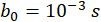 ). Use MATLAB's lsqnonlin solver to minimize the residual norm:
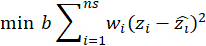
Iterate until convergence (tolerance: ) or maximum iterations (e.g., 1000).
- For linearization of parameter space, rewrite the ELMA equation in matrix form as follows:
- Use the following validation metrics.
- For error quantification, use sum of squared errors (SSE) equation, Root Mean Square Error (RMSE) equation, and . R-squared (R2) equation as given below.
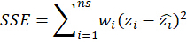


- For error quantification, use sum of squared errors (SSE) equation, Root Mean Square Error (RMSE) equation, and . R-squared (R2) equation as given below.
- Implement the workflow as described below.
- For data acquisition, perform rheological tests under controlled temperatures (e.g., 40 °C, 70 °C) and magnetic fields (0-1.07 T). Export shear stress () and shear rate (
 ) data to MATLAB.
 - For weighting and linearization, apply the weighing scheme described in step 2.3. Construct matrix using initial
 . Perform parameter optimization by solving for using weighted least squares and optimize b using nonlinear least squares.
 - For validation, compare model predictions with experimental data. Calculate RMSE to assess accuracy.
- For data acquisition, perform rheological tests under controlled temperatures (e.g., 40 °C, 70 °C) and magnetic fields (0-1.07 T). Export shear stress (
3. Temperature-compensated damper control implementation
- Temperature-dependent ELMA model development
- For experimental characterization of thermal effects, establish a damper testing setup. Mount a custom MR damper (stroke: 75 mm, piston diameter: 50 mm) on an electro-hydraulic servo machine. Attach a thermocouple to the damper surface for real-time temperature monitoring. Enclose the damper in a temperature-controlled chamber (-30 °C to 80 °C).
- Perform thermal cycling. For each temperature (-30 °C, -20 °C, -10 °C,…,80 °C), apply sinusoidal excitation at amplitude: 40 mm and frequency: 2.085 Hz. Measure the damping force at excitation currents: 0 A, 1 A, 2 A, 3 A. Allow 60 min for temperature stabilization before data acquisition. The experimental setup is shown in Figure 3.
- For parameterization of the ELMA model with current dependency, use the following equation:

where: (dynamic yield stress);
  (post-yield damping coefficient);
  (nonlinear deviation magnitude);
  (exponential decay constant).
 - For quadratic fitting, fit parameters
 , etc, to experimental data using least squares optimization.
- Temperature compensation factor design
- Introduce a temperature-dependent exponential correction factor,
 as follows
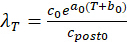
Where = Post-yield damping coefficient at 25 °C,
  = Empirical constants.
 - To determine the modified post-yield damping coefficient, adjust the damping coefficient for temperature effects and update the ELMA model to include thermal correction using the following two equations, respectively.


The expanded form of the equations is

- Introduce a temperature-dependent exponential correction factor,
- Inverse model for real-time current control (Figure 4).
- To make a simplified Bingham-like model, neglect the nonlinear deviation term for real-time control as follows.

The modified expanded form is

- For current calculation, solve the quadratic equation for
 :
:
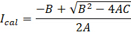
with coefficients:



- For current clamping, apply constraints to
 .
.
- To make a simplified Bingham-like model, neglect the nonlinear deviation term for real-time control as follows.
- Simulation and Validation
- For control surface generation, perform current tracking with inputs: Desired force (
 ), piston velocity (
 ), temperature (
 ) and output: Current command (
 ). Perform force tracking with inputs: Current command (), piston velocity (), temperature () and output: MRD force (
 ).
). - For validation metrics, carry out current tracking accuracy and calculate improvement relative to the uncompensated model (e.g., 3.98% average at 80 °C). Carry out force tracking accuracy and calculate improvement relative to the uncompensated model (e.g., 7.75% average at 80 °C).
- Assess vehicle suspension indicator temperature compensation effect. Use typical quarter suspension (Figure 5) for the simulation of the correlation. The Sky-hook group with compensation control shows a reduction in energy from 1.2504 to 1.1007 on Class D roads, and the Mixed SH-ADD group with compensation control shows a decrease in energy from 1.0565 to 0.9428 on Class D roads. After compensation, the Sky-hook group's absolute value of the peak pitch rate decreased from 6.2775 to 4.0287, and the Mixed SH-ADD group decreased from 6.2776 to 3.6551.
- For control surface generation, perform current tracking with inputs: Desired force (
- Implementation workflow
- For thermal characterization, conduct damper tests across temperatures (-30 °C to 80 °C). Export force-velocity data for parameter fitting.
- For model parameterization, fit ELMA model parameters (,etc.) using MATLAB's lsqcurvefit. Determine constants (
 ) via nonlinear regression.
 - For inverse model deployment, implement the model in Simulink with saturation blocks for current clamping.
- For validation, check tracking accuracy (Figure 6 and Figure 7). Compare the compensated and uncompensated vehicle suspension system responses (Figure 8 and Figure 9).
Access restricted. Please log in or start a trial to view this content.
Results
The temperature compensation strategy presented in this protocol focuses primarily on magnetorheological dampers, and the compensation control is determined from comprehensive tests at the damper level over a range of current, velocity, and temperature dependencies. However, we also did the magnetorheological fluid-related temperature experiments to obtain the image shown in Figure 10, when the temperature is higher than 0 °C, we can see that the change rule ...
Access restricted. Please log in or start a trial to view this content.
Discussion
The protocol provides a structured approach to address the temperature sensitivity of magnetorheological (MR) dampers through three interrelated innovations: optimized magnetorheological fluid synthesis, exponential linear mixing analysis (ELMA) modeling, and adaptive temperature compensation algorithms. Key steps include gradient-based homogenization of the magnetorheological fluid with sequential addition of additives at a controlled temperature (50 ± 2 °C) to minimize particle deposition. The original parame...
Access restricted. Please log in or start a trial to view this content.
Disclosures
The authors have no financial interests in the products described in this manuscript and have nothing else to disclose.
Acknowledgements
This work was supported by the National Natural Science Foundation of China [grant numbers 51761135124, 11672148, 52003142, 51775293]; and the State Key Laboratory of Vehicle NVH and Safety Technology [Grant number NVHSKI-202106]
Access restricted. Please log in or start a trial to view this content.
Materials
| Name | Company | Catalog Number | Comments |
|---|---|---|---|
| air compressor | Dynair | DA5002CS | |
| Carbonyl Iron Powder | BASF | CIP-SQ | |
| Electro-hydraulic servo fatigue testing machine | DOCER | PWS-1000 | |
| MATLAB | Mathworks | R2022b | |
| Organic bentonite | ELEMENTIS | - | |
| Poly-alpha-olefin | INEOS | PAO162 | |
| Propylene carbonate | MACKLIN | PC | |
| Rheometer | Anton Paar | MCR702 | |
| Surfactant | Jinzhou Xinxing | T154A | |
| temperature control platform | Peltier | H-PTD200 |
References
- Deng, L., et al. Design of a Dual-Motor Powertrain with Magnetorheological Planetary Transmission for Electric Vehicles 2024-01-2636. SAE Technical Paper. , (2024).
- Seo, Y. P., et al. Searching for a stable high-performance magnetorheological suspension. Adv Mater. 30 (42), 1704769(2018).
- Hajalilou, A., Mazlan, S. A., Lavvafi, H., Shameli, K. Field responsive fluids as smart materials. , Springer. (2016).
- Gołdasz, J., Sapiński, B. Insight into magnetorheological shock absorbers. , Springer International Publishing. Switzerland. (2015).
- Zhu, X., Jing, X., Cheng, L. Magnetorheological fluid dampers: A review on structure design and analysis. J Intelligent Mater Syst Struct. 23 (8), 839-873 (2012).
- Yang, G., Spencer, B. Jr, Carlson, J., Sain, M. Large-scale mr fluid dampers: Modeling and dynamic performance considerations. Eng Struct. 24 (3), 309-323 (2002).
- Sheikh, H., Van Engelen, N. C., Ruparathna, R. A review of base isolation systems with adaptive characteristics. Structures. 38, 1542-1555 (2022).
- Guglielmino, E., Sireteanu, T., Stammers, C. W., Ghita, G., Giuclea, M. Semi-active suspension control: Improved vehicle ride and road friendliness. , Springer Science & Business Media. (2008).
- Zhu, Z., Zhang, X. Damping performance optimization of the magnetorheological damper with three parallel channels. Structures. 44, 1962-1973 (2022).
- Hadadian, A., Sedaghati, R., Esmailzadeh, E. Design optimization of magnetorheological fluid valves using response surface method. J Intelligent Mater Syst Struct. 25 (11), 1352-1371 (2014).
- Kazakov, Y. B., Morozov, N., Nesterov, S. Development of models of the magnetorheological fluid damper. J Magnetism Magnetic Mater. 431, 269-272 (2017).
- Bitman, L., Choi, Y. T., Wereley, N. M. Passive damping and isolation. Proc SPIE. 3045, (1997).
- Guo, P., Guan, X., Ou, J. Physical modeling and design method of the hysteretic behavior of magnetorheological dampers. J Intelligent Mater Syst Struct. 25 (6), 680-696 (2014).
- Guo, S., Yang, S., Pan, C. Dynamic modeling of magnetorheological damper behaviors. J Intelligent Mater Syst Struct. 17 (1), 3-14 (2006).
- Wereley, N. M., Pang, L., Kamath, G. M. Idealized hysteresis modeling of electrorheological and magnetorheological dampers. J Intelligent Mater Syst Struc. 9 (8), 642-649 (1998).
- Wang, D., Liao, W. Modeling and control of magnetorheological fluid dampers using neural networks. Smart Mater Struct. 14 (1), 111(2004).
- Wang, D., Liao, W. H. Magnetorheological fluid dampers: A review of parametric modelling. Smart Mater Struct. 20 (2), 023001(2011).
- Xu, Z. D., et al. Force tracking model and experimental verification on a novel magnetorheological damper with combined compensator for stay cables of bridge. Structures. 32, 1971-1985 (2021).
- Bui, Q. D., Bai, X. X., Nguyen, Q. H. Dynamic modeling of mr dampers based on quasi-static model and magic formula hysteresis multiplier. Eng Struct. 245, 112855(2021).
- Batterbee, D., Sims, N. Active and Passive Smart Structures and Integrated Systems. Proc SPIE. 12043, 360-370 (2008).
- Liu, Y., et al. Smart Structures and Materials 2003: Industrial and Commercial Applications of Smart Structures Technologies. Proc SPIE. 5054, 332-340 (2003).
- Wilson, N. L., Wereley, N. M., Choi, Y. -T., Hiemenz, G. J., Hu, W. Active and Passive Smart Structures and Integrated Systems 2009. Proc SPIE. 7288, 318-327 (2009).
- Priya, C. B., Gopalakrishnan, N. Temperature dependent modelling of magnetorheological (mr) dampers using support vector regression. Smart Mater Struct. 28 (2), 025021(2019).
- Choi, S. B. Thermal conductivity and temperature dependency of magnetorheological fluids and application systems-a chronological review. Micromachines. 14 (11), 2096(2023).
- Zhu, H., Rui, X., Yang, F., Zhu, W., Jiang, M. Influence of temperature and internal leakage on magnetorheological damper. Int J Mech Syst Dynamics. 4 (4), 487-496 (2024).
- Influence of Temperature on the MR Squeeze-Mode Damper. Gołdasz, J., Sapinski, B. Proc 2019 20th Int Carpathian Cont Conf, , 1-6 (2019).
- Yu, J., Dong, X., Wang, X., Pan, C., Zhou, Y. Asymmetric dynamic model of temperature-dependent magnetorheological damper and application for semi-active system. Front Mater. 6, 227(2019).
Access restricted. Please log in or start a trial to view this content.
Reprints and Permissions
This article has been published
Video Coming Soon