Two-color Multifiber Photometry Recordings of the Social Behavior Network in Mice

Summary

Fiber photometry is one of the most common techniques used to record calcium activity from deep-brain neural populations. Here, we describe a protocol for customizable, multisite two-color imaging of calcium activity and other dynamic fluorescent signals from deep-brain neural populations in mice.

Abstract

Fiber photometry, the bulk recording of signals through a fiber optic cable, is a useful method for recording calcium activity from groups of neurons in the freely moving rodent. In particular, this method makes targeting small populations of genetically specified neurons in more ventral and less accessible areas of the brain a tractable problem, since it remains challenging to record at cellular resolution. This technique can be scaled to record from multiple sites simultaneously using a bundled multifiber approach and can target multiple cell types using genetic strategies at each recorded site. Here, we provide a protocol for how to build and insert customized multifiber arrays for targeting the mouse social behavior network (up to 12 sites). This protocol details the surgical operating procedures required for successful targeting of multiple sites using our customized multifiber arrays and the viral approach for delivery of green- and red-shifted fluorescent indicators of calcium activity for simultaneous imaging of two genetically identified neural populations at each site. We demonstrate how to record from these regions using a commercially available complementary metal-oxide semiconductor (CMOS) camera system during social behavior. Further, this protocol demonstrates methods for quality control and details a preprocessing pipeline for noise correction and standardization. Finally, we discuss some potential applications of the tool to uncover novel findings about large-scale brain networks.

Introduction

Fiber photometry, the bulk recording of fluorescent signals through fiber optic cables, has emerged as a powerful technique for measuring neural population activity in deep-brain regions. Often, these regions are not easily accessible with microendoscopy or traditional electrophysiological approaches^1,2,3. A major goal in contemporary systems neuroscience is to identify and unravel the computations employed by large-scale, cell-type-specific brain networks involved in the generation of behavior. Neuropixel probes and commercially available multifiber ferrules excel at recording from linearly aligned neural populations^4,5,6,7, while widefield cortical imaging provides excellent coverage of superficial cortical dynamics^8,9. However, recording simultaneously from spatially dispersed yet functionally connected subcortical neural populations has remained technically challenging^5,10,11,12. Further, while it is possible to target multiple deep-brain structures using multiple single-fiber ferrules for photometry, this approach is limited to neural populations sufficiently distal from each other for multiple ferrules to be implanted¹². Bespoke multifiber photometry arrays address this gap by enabling simultaneous recordings from many subcortical regions in freely behaving animals with minimal constraints, providing a unique window into network-level coordination during complex behaviors.

The social behavior network (SBN) represents an ideal system for investigating large-scale brain network dynamics. The SBN is a densely interconnected and evolutionarily conserved set of subcortical structures involved in the generation of social behavior that has been identified across all vertebrate classes^13,14,15. These structures traditionally include, but are not limited to, the lateral septum, preoptic area, bed nucleus of the stria terminalis, anterior and ventromedial hypothalamic nuclei, the medial amygdala, nucleus accumbens, and periaqueductal gray^13,14,15. Within the SBN, specific neural populations defined by molecular markers play critical roles in social behavior regulation. SBN ɣ-aminobutyric acid-ergic (GABAergic) neurons (marked by the expression of the vesicular GABA transporter, or VGAT) and glutamatergic neurons (marked by expression of the vesicular glutamate transporter, or VGlut) represent the major excitatory and inhibitory cell types within the network and likely play dissociable roles in the modulation of social action^16,17,18,19. Beyond these classical neurotransmitter systems, sex hormone signaling plays a critical role in the network’s function. For example, many male and female social behaviors require the expression of estrogen receptor alpha, and activity in SBN neurons expressing these receptors causally drives these behaviors^{16,20,21,22,23,24,25,26}. In addition, SBN neural populations are enriched with ligands and receptors of many neuromodulatory systems, including dopamine, arginine vasopressin, oxytocin, opioids, tachykinin, neuropeptide Y, prolactin, orexin, agouti-related peptide, melanocortins, kisspeptin, and gonadotropin-releasing hormone^{17,18,19,27,28,29,30,31}, and recent advances in genetically encoded sensors now permit tracking of many of these diverse signaling molecules^{32,33,34,35,36,37,38}. Because SBN neural populations are spatially dispersed throughout subcortical structures, traditional experimental preparations (e.g., extracellular electrophysiology, cortical surface imaging, and earlier approaches to multifiber photometry) are unable to capture the moment-to-moment activity dynamics across this large-scale brain network. Nevertheless, by monitoring calcium dynamics in genetically defined neural populations alongside neuromodulator release patterns, bespoke multisite fiber photometry platforms can reveal which specific cell types and signaling molecules encode particular features of social behavior, providing novel mechanistic insights.

Here, we developed a customizable platform for multisite, two-color fiber photometry that enables simultaneous recording from up to 12 brain regions in freely behaving mice. Using this approach, we performed two-color photometry recordings of calcium activity from 22 identified neural populations distributed across 11 SBN brain regions, alongside measurements of dopamine fluctuations in the nucleus accumbens with a GPCR-activation-based-DA sensor (GRAB-DA1m)³³ (Table 1). This protocol (Figure 1) details the construction of customized multifiber arrays, surgical procedures for targeting multiple deep-brain sites, viral delivery strategies for expressing dual calcium indicators (GCaMP³⁹ and RCaMP⁴⁰), data acquisition using a commercially available CMOS camera-based fiber photometry system, quality control methods, and a preprocessing pipeline for noise correction and signal standardization. Critically, our preprocessing pipeline incorporates isosbestic control wavelength recordings which enable us to perform motion artifact correction. We take a regression-based approach⁴¹ to correct for motion artifacts, ensuring signal fidelity during vigorous social behaviors such as mounting or fighting. As our bespoke multifiber photometry method can simultaneously monitor activity dispersed across both proximal and distal deep-brain structures while maintaining cell-type specificity of the recordings through genetic targeting^42,43, it offers significant advantages over alternative approaches to recording neural activity dynamics across deep-brain, large-scale brain networks.

This protocol is optimally suited for experiments requiring simultaneous recordings from spatially dispersed subcortical brain regions (≥4 sites) in freely behaving animals, particularly when investigating network-level dynamics across genetically defined cell types or tracking neuromodulator release alongside neural activity. The approach is especially valuable for studying naturalistic behaviors involving vigorous movement (e.g., social interactions), where our motion artifact correction pipeline ensures signal fidelity. However, researchers seeking single-cell resolution, distinction between somatic and axonal signals, or recordings from superficial cortical regions may find alternative approaches (e.g., miniature microscopy, Neuropixels, or widefield imaging) more appropriate. Key practical considerations include surgical complexity, the need for custom multifiber array fabrication, and establishing the requisite materials infrastructure (3D printing capabilities, fiber optic tools).

Protocol

NOTE: This protocol was tested and validated using adult mice aged 8–25 weeks. Mice were housed at 21–26 °C and 30%-70% humidity in a 12-h reversed dark-light cycle (OFF: 10:00 AM; ON: 10:00 PM). Experiments occurred exclusively during the subjective active (dark) phase. Food and water were provided ad libitum. All animal procedures were approved by the Princeton University Institutional Animal Care and Use Committee and were in accordance with National Institutes of Health Standards.

1. Multifiber Array and Patchcord Fabrication (Figure 1A)

1. Fabricate patchcord (Figure 2A).
   1. Obtain a 12 fiber-branching patchcord and print the provided patchcord connector and stereotactic drilling accessories (Supplemental File 1, Supplemental File 2, Supplemental File 3) using resin (tensile strength: 8.7 kilopound/square inch [ksi], e-module: 377 ksi, heat deflection: 138 °F, elongation: 8%).
   2. Build the provided polishing puck (Supplemental File 4) out of a 2-inch diameter stainless steel rod and include a cutout of the multifiber array’s size in the center of the puck.
   3. Manually clear the excess resin out of the dowel pin through-holes in the multifiber array with a 1.22 mm x 11mm drill bit. Even with precision 3D printing, dowel pin holes are slightly too small for the dowel to go through.
   4. Drill fiber through-holes.
      1. Insert alloy steel dowel pins (1.19 mm x 12.7 mm) into all 4 pin holes in the stereotactic drilling accessory and place the patchcord connector bottom-side up into the stereotactic drilling accessory with the dowel pins going through the multifiber array’s dowel pin through-holes.
      2. Tighten size M4 set screws in the threaded screw holes to secure the patchcord connector in place and secure stereotactic drilling accessory into the stereotactic frame.
      3. Insert a 0.25 mm x 5.5 mm drill bit into the stereotactic drill and mount the drill to the stereotactic frame. Using this drill bit, level the yaw, pitch, and roll of the multifiber array with a maximum deviation tolerance of ±0.03 mm.
         NOTE: Level yaw and pitch at the most anterior and posterior positions of the 3D print, level roll at the four corners of the multifiber array.
      4. Center drill above one of the 3D printed fiber holes and set the stereotactic frame X/Y coordinates to the ML (X) and AP (Y) coordinates of the associated brain region (Table 1). Move drill to the new (0, 0) coordinates on the stereotactic frame to center the drill above the anterior dowel pin through-hole.
      5. Use the 0.25 mm x 5.5 mm drill bit to drill out each fiber through-hole to a depth of 5.5 mm at the stereotactically defined coordinates (Table 1).
         NOTE: Use a long piece of excess fiber to check that all holes are fully cleared before removing the multifiber array from the stereotactic frame. This will limit the number of times the multifiber array will need to be leveled and drilled to clear out the through holes.
   5. Adjoin the patchcord connector and branching patchcord
      1. Expose >10 cm of the patchcord fibers. Trim fibers with a fiber scribe to ensure they are of equal length. Then, place a single piece each of 3/16” and 5/16” heat shrink tubing around the 12 fibers on the patchcord.
         NOTE: The tubing will protect any exposed fibers after they are glued into the connector.
      2. Insert each fiber into one of the through-holes in the patchcord connector such that approximately 0.3 mm of fiber is exposed at the bottom surface. After inserting all the fibers, use a 21–27 G needle tip to apply superglue to top surface of the patchcord connector to fix the fibers in place.
      3. Apply epoxy to the top surface of the patchcord connector in a 0.5–1 cm tall pyramid shape. Ensure no epoxy covers any area besides the top-surface where the fibers were inserted. Allow epoxy to cure at room temperature overnight.
      4. Use a heat gun at the lowest setting to shrink the heat shrink tubing over the epoxy and exposed fiber above it (<3–5 cm).
         NOTE: Avoid touching the heat shrink tubing while doing this to prevent burns.
      5. Cut a piece of soft plastic tubing with a 3 mm inner diameter to the length of the remaining exposed fibers, cut slit along the edge of the tubing, and encase the remaining exposed fiber in the tubing.
      6. Color the clear tubing with an opaque black marker to ensure that the fibers are no longer visible, minimizing illumination from exposed fiber during imaging experiments.
   6. Polish the patchcord.
      1. Secure patchcord connector bottom-surface down in the custom polishing puck. Polish the patchcord connector on 6 µm, 3 µm, 1 µm, and then 0.01 µm grit polishing sheets with 10–20 motions in the shape of the infinity symbol/sheet. For the 1 µm and 0.01 µm grit sheets, place 5 drops of distilled water prior to polishing.
      2. Wipe the surface of the connector to rid any excess distilled water. Check for fiber blemishes or cracks on the polished surface side of the patchcord connector using a brightfield microscope, and, if any exist, repeat polishing.
   7. Check patchcord output.
      1. Connect the Sub-miniature version A (SMA) connector end of the patchcord to a CMOS camera-based fiber photometry imaging system. Using visual coding software, follow the photometry imaging system’s manual and focus the CMOS camera on the SMA end of the patchcord.
         NOTE: The manual is updated regularly to align with software updates. As the visual code for the photometry system often changes with new software releases, this manual contains the most up-to-date information for current software releases.
      2. Measure 470 nm patchcord output at 20% power with an optical power meter. Repeat step 1.1.7 if patchcord output is < 2.5 mW.
2. Fabricate Multifiber Array.
   1. Print the provided multifiber array (Supplemental File 5, Supplemental File 6) using resin with the technical specifications described in step 1.1.1.
   2. Prepare multifiber array.
      1. Insert M0.6 Brass Hex nuts into each of the four slots in the side corners of the multifiber array and align the hole of the hex nut into the center of the opening.
      2. Apply a single drop of super glue from the side of each hex nut slot with a 21–27 G needle tip, adding additional drops for reinforcement if necessary. Allow the glue to dry at room temperature for 5 min before moving to the next step.
      3. Shave away any glue on the sides of the multifiber array using a razor blade to ensure it fits into the polishing puck.
      4. If excess superglue dried on the surface-side of the multifiber array, polish the multifiber array’s surface using the custom polishing puck and 30 µm grit polishing sheets until glue is removed and the multifiber array surface is flat.
      5. Manually clear the excess resin out of the dowel pin through-holes in the multifiber array with a 1.22 mm drill bit.
   3. Drill out fiber-through holes (Figure 2B-C).
      1. Insert alloy steel dowel pins (1.19 mm x 12.7 mm) into all 4 pin holes in the stereotactic drilling accessory and place the multifiber array surface-side (flat-side) up into the stereotactic drilling accessory with the dowel pins going through the multifiber array’s dowel pin through-holes.
      2. Repeat step 1.4.2– step 1.4.5.
   4. Prepare fibers for the multifiber array.
      1. Strip the plastic casing off a section of 200 µm, 0.39 NA optic fiber using a fiber stripper. Clean the fiber with ethanol.
      2. Cleave the fibers into ~3–5 cm long sections using a fiber cleaver. Further cleave these sections in half using a fiber scribe. Use a brightfield microscope to ensure that at least one end of the cleaved sections is without chips or blemishes. Only use fibers with at least one unblemished end.
      3. Tape a precise ruler of at least 15 mm in length under the brightfield microscope. Place the unblemished side of the fiber at the 0 mm position on the ruler (Figure 2D). Cut fibers to desired length for each targeted region (Table 1).
         NOTE: Fiber length is calculated by adding 6 mm to the stereotactic D/V coordinate for the deepest fiber, and then adjusting that value for all fibers to match the difference between their D/V coordinate and the deepest fiber’s D/V coordinate.
   5. Insert fibers into the multifiber array.
      1. Place the multifiber array into the fabrication holder surface-side down. Align and secure the piece using dowel pins.
      2. Match fiber length to site (Table 1) and insert cleaved fibers into the appropriate through-holes in the multifiber array with the unblemished side facing up. Ensure that all fibers are pushed all the way in before the next step.
      3. Apply superglue with a 21–27 G needle tip to glue all fibers into place. Allow the glue to drive for a minimum of 30 min at room temperature before continuing.
   6. Polish the multifiber array by repeating step 1.1.6 with multifiber array surface-side down (Figure 2E).
   7. Check multifiber array efficiency.
      1. Clean the polished surface of the multifiber array with ethanol and then apply index matching gel to it. Insert 4 dowel pins into the patchcord connector and secure the multifiber array to it using G5 drive screws and associated screwdriver (Figure 2F).
      2. Use a powermeter to measure 470 nm and 560 nm LED emission from the multifiber array. Compute efficiency using these values:
         
      3. If efficiency is <75%, repeat steps 1.2.7.1–1.2.7.2.
         NOTE: If re-polishing does not improve the efficiency and there are no blemishes on the fibers, it is possible that the fibers on the multifiber array are off alignment to the patchcord connector.
   8. Prepare multifiber array for use (Figure 2G).
      1. Insert 4 dowel pins into the through-holes in the multifiber array. Ensure that the dowel pins do not stick out more than 1mm from the brain-side of the multifiber array.
      2. Place superglue brain-side on the dowel pins. Allow the glue to dry for at least 10 min at room temperature before using the multifiber array.

2. Surgery (Figure 1B)

1. Prepare surgical space and tools.
   1. Clean stereotactic frame to ensure an aseptic working area.
   2. Obtain sterile absorbable suture.
   3. Autoclave a pair of fine forceps, fine scissors, and two bulldog clamps.
   4. Ensure the vaporizer is filled with isoflurane. Ensure that the tubing for the isoflurance, vacuum, and oxygen lines are securely connected to the vaporizer, induction chamber, and the stereotactic frame’s nose cone.
2. Obtain jRCaMP1b, GCaMP6f, and GRAB-DA1m adeno-associated viruses.
   CAUTION: Always wear personal protective equipment while handling viruses.
   1. Dilute viruses to a working concentration of between 1x10¹³ and 4x10¹³ parts/milliliter if necessary.
   2. Prepare a 1:1 mixture of jRCaMP1b and GCaMP6f adeno-associated viruses.
   3. Place an aliquot of the 1:1 jRCaMP1b:GcaMP6f viral mixture and an aliquot of GRAB-DA1m virus on ice to maintain temperature at 4 °C.
3. Induce anesthesia.
   1. Place the mouse into the induction chamber and close the chamber door. Start the flow of oxygen into the vaporizer at 1 L/min.
   2. Direct the gas flow into the induction chamber and turn on the vacuum line to remove excess gas from the chamber. Set the vaporizer to an isoflurane concentration between 3% – 5%.
4. Transfer mouse to stereotactic frame.
   1. Once the mouse’s breathing has slowed to 1 breath/s, move the mouse onto the stereotactic frame. Hook the mouse’s front incisors into the slot in the nose cone’s mouthpiece and tighten the nose cone over the mouse’s nose.
   2. Switch the gas flow to the stereotactic frame with the isoflurane concentration set to 1%–2% to maintain anesthesia. Switch the vacuum line to remove gas from the nose cone.
      ​NOTE: Monitor the mouse’s breathing throughout surgery and adjust the isoflurane concentration as needed to maintain deep anesthesia with a breathing rate of 1 breath/s. Deep anesthesia should be confirmed periodically throughout surgery by ensuring the mouse is unresponsive to a toe pinch.
   3. Set the heating system to maintain a body temperature of 35 °C and apply optic ointment to the mouse’s eyes to prevent them from drying out.
   4. Insert stereotactic ear bars so they push on either side of the skull, slightly dorsal and anterior to the ear canals. Tighten ear bars and ensure the mouse’s skull is fixed in place by applying gentle pressure to the top of the mouse’s head.
5. Prepare the scalp for incision.
   1. Trim or shave the hair on top of the mouse’s head until it is short. Apply hair removal gel onto the top of the mouse’s head and let sit for approximately one minute. Remove remaining gel with a clean cotton swab.
   2. Repeat 2.5.1 as needed until all hair on the top of the head has been removed.
   3. Disinfect the skin on top of the head by using cotton swabs to apply betadine (10% povidone-iodine solution) followed by 70% ethanol solution.
6. Expose the skull.
   1. Cut an incision along the midline of the skull, extending from slightly posterior of lambda to slightly anterior of the rostral rhinal vein.
      NOTE: The rhostral rhinal vein is the blood vessel which sits on the dorsal surface of the brain between the olfactory bulb and prefrontal cortex.
   2. Cut and remove shaved skin around the sides of this incision to form a tear-drop shaped cut that exposes the parietal bones, the anterior tip of the intraparietal bone, and the portion of the nasal bones that is anterior to the rostral rhinal vein (Figure 2H).
   3. Gently clean the skull surface with 0.9% saline solution and a clean cotton swab.
7. Level the skull.
   1. Locate where the rostral rhinal vein meets the sagittal suture. Mark this point with a sterile scalpel blade.
   2. Insert a #92 carbide drill bit into the stereotactic drill and mount the drill on the stereotactic frame. Use the stereotactic manipulator to position the tip of the drill on the skull surface at the marked point and zero the drill’s X, Y, and Z coordinates.
   3. Level pitch of the skull by measuring Z depth at the marked point and -8.25 mm posterior to it. Level yaw of the skull by measuring the lateral distance between the marked point and the position -8.25 posterior. Level roll by measuring Z depth at positions ±2.0–2.5 mm from the midline at positions -2.0, -4.5, and -7.0 mm relative to the marked point.
8. Perform craniotomies and duratomies.
   1. Replace drill bit with a #76 or #78 carbide drill bit. Zero the drill at the marked position at the junction of the sagittal suture, rostral rhinal vein, and skull surface.
   2. Move the drill to each brain region’s A/P and M/L coordinates (Table 1). At each site, drill a craniotomy and carefully remove the dura mater at each craniotomy using a 27G or smaller empty syringe tip.
9. Inject the virus.
   1. Pull glass micropipettes such that their tip tapers for at least 7 mm and has a tip opening of 10–30 µm.
      NOTE: Restart steps 2.9.2–2.9.12 if the micropipette contains any air bubbles after any of the subsequent steps.
   2. Backfill an empty glass micropipette tip with mineral oil. Insert and secure micropipette tip into the nanoliter injector. Use the nanoliter injector interface to eject as much mineral oil from the micropipette as possible.
   3. Mount the nanoliter injector onto the stereotactic frame. Cut a small piece of paraffin wax sheet and place it on the mouse’s head.
   4. Pipette 1 µL of the jRCaMP1b:GCaMP6f virus mixture onto the paraffin wax. Lower the tip of the nanoliter injector so the glass micropipette tip is in the virus mixture and backfill the micropipette with virus using the injector’s interface.
   5. Repeat 2.9.4 until all virus that will be used has been transferred to the nanoliter injector (Table 1). Remove and dispose of the paraffin wax in a biohazard waste container.
   6. Zero the injector micropipette tip at the marked position at the junction of the sagittal suture, rostral rhinal vein, and skull surface.
   7. Starting with the most ventral to most dorsal injection site (Table 1), move the micropipette tip to each site, lower it to touch the brain surface, and zero the Z-position on the stereotactic frame.
   8. At each site, lower the micropipette tip into the brain until it is 0.1 mm ventral relative to the injection site. Then, raise the micropipette tip 0.1 mm to the final injection site. Allow the surrounding tissue to settle around the micropipette tip for 30 s.
   9. Using the nanoliter injector interface, inject 300 nL of the 1:1 jRCaMP1b:GcaMP6f virus mixture at a rate of 1–2 nL/s to disperse the mixture at the current injection site.
   10. Allow the micropipette tip to remain at the injection site for at least 5 min following injection completion. Slowly raise the micropipette tip out of the brain to reduce risk of virus spreading dorsally along the injection track.
   11. After injecting the 1:1 jRCaMP1b:GcaMP6f viral mixture at each site, use the nanoliter injection interface to return the plunger of the nanoliter injector to its original position. Remove the micropipette and dispose of it in a biohazard sharps waste container.
   12. If necessary, repeat steps 2.9.2–2.9.11 for each brain region targeted for GRAB-DA1m expression. At each targeted site, inject 150 nL instead of the 300 nL used for the virus mixture.
10. Implant multifiber array.
    1. Secure the multifiber array to the stereotactic frame using any attachment that can hold the multifiber array by the dowel pins to keep it stable during implantation (Figure 2I).
    2. Adjust the multifiber array’s position such that each fiber aligns with the center of its respective craniotomy and with the longest fiber resting at the brain surface. Zero the stereotactic manipulator at this location and slowly lower the multifiber array until it is 0.25 mm above the D/V position of the deepest virus injection (Table1, Figure 2J).
    3. Place a cold mixing dish on ice and add to it 1 scoop of cement powder, 4 drops of liquid base, and 1 drop of catalyst. Mix for 20 s.
       NOTE: Repeat this step whenever liquid cement is used and more is required.
    4. Use a syringe and 23–31 G needle to transfer liquid cement in the space between the multifiber array and the skull.
    5. Apply liquid cement using a thin plastic applicator or syringe needle to fully cover the four sides of the multifiber array, building up a pyramid like shape from the skull (Figure 2K). Allow the cement to dry for at least 15 min.
    6. Suture the skin together along the incision to ensure no skull is exposed.
11. Allow mouse to recover.
    1. Reduce isoflurane concentration to 0.
    2. Transfer mouse from stereotactic frame to a heating pad and wait for mouse to be alert and ambulatory before transferring it back to its cage.
    3. Allow the mouse to recover for at least two weeks before beginning experiments.

3. Multisite, Two-color Calcium Imaging (Figure 1C)

1. Configure Data Acquisition Device (DAQ).
   1. Connect the GND to the AGND port above the Ch7 port using electrical wire.
   2. Connect the DIO0 to the Ch0 port using electrical wire.
2. Connect the photometry system to the DAQ.
   1. Attach the Baby Neill Constant (BNC) connector end of a split BNC cable (BNC connector at one end, red and black electrical wires at the other end) to the input port on the photometry system. Attach the BNC connector end of another split BNC cable to the output port on the photometry system.
   2. Take the split BNC cable connected to the photometry system’s input port and connect its red wire end to the DIO1 port on the DAQ. Take the split BNC cable connected to the photometry system’s output port and connect its red wire end to the Ch1 port on the DAQ.
   3. Connect the black ground wires from both split BNC cables to the DAQ GND port.
3. Synchronize behavior and photometry cameras.
   1. Daisy-chain multiple behavior cameras together for simultaneous recordings of behavior from multiple angles.
      1. Connect the opto-isolated output (pin 4, white wire) of the primary behavior camera to the secondary camera’s non-isolated input (pin 1, green wire) with a 3.3 KΩ resistor. Connect the primary camera’s 3.3 V output (pin 3, red wire) to the same 3.3 KΩ resistor and to Ch2 on the DAQ.
      2. Connect the opto-isolated output of each secondary camera to its 3.3 V output using a 3.3 KΩ resistor.
      3. Connect the primary camera’s ground (pin 6, brown wire) to each secondary camera’s ground. Connect all camera ground wires to the DAQ AGND port above the Ch2 port and to the photometry system’s output ground.
4. Configure behavior camera settings using the associated imaging software.
   1. Set the “Acquisition Frame Rate” to 45 Hz and the gain to 1.
   2. Set the exposure time to 2998 µs, exposure lower limit to 100 µs, and exposure upper limit to 150000 µs.
      NOTE: “Acquisition Frame Rate” may not be the actual frame rate that will be captured. Depending on the exposure time and requested data bandwidth, this value may need to be set higher than the final imaging frequency. If necessary, adjust “Acquisition Frame Rate” such that the displayed “Resulting Frame Rate” is 40 Hz.
5. Configure DAQ software (Supplemental File 7).
   1. In the DAQ software, add the DAQ as a ‘Device’ and switch to the ‘Configuration Panel’.
   2. In the ‘Channels’ tab, under ‘Analog Input’, activate channels 0–2. Under ‘Digital’, activate channel 0.
      NOTE: Ch0 corresponds to the transitor-transitor logic (TTL) signal, Ch1 to the photometry system, and Ch2 to the daisy-chained cameras.
   3. Under ‘Analog Input’, name channel 0 “TTL”, channel 1 “Photometry_system”, and channel 2 “Behavior_cameras” which stands for “Transitor-Transistor Logic”. Under ‘Digital’, name channel 0 “TTL_trigger”.
   4. In the ‘Triggers’ tab, set triggers to manual. In the ‘Sample Rates’ tab, set the sample rate to 350 Hz.
   5. Switch to the ‘Display Panel’ and put the ‘Strip’, ‘Scalar’, and ‘Output’ windows into the graphical user interface.
6. Configure photometry system software (Supplemental File 8).
   1. Develop a workflow in the visual coding software to accept a 5 V TTL pulse to trigger the recordings and to save the timestamp for each frame, the fluorescence emissions for the red and green channels for each fiber, and the raw video, as outlined in the photometry system manual.
   2. Using the node for the photometry system in the workflow, ensure that the system is set up to record alternating frames of 560, 470, and 415 nm LED at 120 Hz for a functional framerate of 40 Hz.
      NOTE: This time-division multiplexing (TDM) approach addresses spectral overlap between GCaMP and RCaMP by temporally separating their excitation, ensuring that each indicator is excited independently across consecutive frames. The recording system employed here uses optimized bandpass emission filters (green channel: 500–530 nm; red channel: >580 nm longpass) that further minimize spectral crosstalk by restricting detected photons to wavelengths predominantly emitted by each indicator. The 415 nm isosbestic wavelength excites both GCaMP and RCaMP equally but produces minimal calcium-dependent fluorescence changes, providing a motion artifact control signal. Together, TDM excitation and spectral filtering ensure that 470 nm frames capture predominantly GCaMP activity (Figure 3A), 560 nm frames capture predominantly RCaMP activity (Figure 3B), and 415 nm frames provide calcium-independent reference signals for motion correction.
7. Perform in vivo photometry recordings.
   1. Obtain mouse that underwent viral injections and multifiber array implantation as outlined in Step 2.
   2. Clean the connection surfaces of the patchcord and implanted multifiber array with ethanol and a cotton swab. Using the node for the photometry system in the visual coding workflow and a photometer, set each of the 415, 470, and 560 LED power levels to output approximately 1.2 mW of illumination from the patchcord.
   3. Apply index matching gel to the connection surface of the patchcord. Align the patchcord to the mouse’s implanted multifiber array with the array’s dowel pins, and slide patchcord down until flush with the surface of the implanted multifiber array.
   4. Tighten patchcord screws to secure the multifiber array into the patchcord. Let the mouse habituate before beginning experiments (Figure 2L–M).
   5. Set file names.
      1. For each behavior camera, press the red circle ‘record’ button to open its recording window in the behavior camera recording software and specify its filename.
      2. Open the DAQ software program, click the gear button and navigate to ‘logging options’, and specify the filename.
      3. Click on the ‘PhotometryWriter’ node of the photometry system visual coding workflow to specify the filename.
   6. In the behavior camera software recording windows, click ‘start recording’ for each camera. Next, press the play button in the photometry system visual coding workflow, and press record in the DAQ software.
   7. Click the TTL switch to begin recording synchronously across all cameras.
   8. End recording.
      1. Click the TTL switch to end synchronous camera recordings
      2. Press the stop button in the visual coding workflow for the photometry system, “stop recording” in the behavior camera software recording windows.
   9. Repeat steps 3.7.5–3.7.8 until end of experiments, and disconnect the mouse.
      NOTE: Following experiments, photometry and behavior camera data streams can be aligned with custom code using the output of the DAQ software. Specifically, (1) the change in TTL voltage indicates the time of TTL onset and offset, (2) changes in behavior camera voltage indicate when when the camera shutter opens and closes to capture each frame of behavior video, and (3) the initial change in photometry system voltage recorded on the DAQ can be compared to the TTL onset time and the photometry camera timestamps output from the visual coding software to determine the photometry camera timestamps.

4. Data processing (Figure 1D, Supplemental File 9)

1. Preprocess calcium imaging data.
   1. De-interleave frames of calcium imaging data to create separate streams of signal recorded in response to 415 nm, 470 nm, and 560 nm LEDs.
   2. Use the Adaptive Iteratively Reweighted Penalized Least Squares algorithm (airPLS)⁴⁴ to correct for baseline drift.
   3. Compute ΔF/F using:
      
      NOTE: The baseline period should be a stable epoch before experimental manipulation (e.g., before introducing a social partner). If the baseline period is too short (<2–3 min) or exhibits large fluctuations that may be contaminated by motion artifacts, consider normalizing using the mean fluorescence across the entire session instead of a restricted baseline period.
2. Correct for motion artifacts (Figure 4A).
   1. Use a regression-based approach, although alternative methods are suitable (see Table 2)
   2. Z-score ΔF/F signals using the median to normalize signal magnitude across regions:
      
   3. Apply Lasso regression with L1 regularization. Lasso (Least Absolute Shrinkage and Selection Operator) performs automatic feature selection by shrinking coefficients of uninformative predictors toward zero.
      1. Perform grid search across regularization parameters (α = 0.0001, 0.001, 0.01, 0.1, 1, 10, 100). The grid search identifies the optimal balance between model complexity and overfitting. This step can be fully automated using cross-validation routines available in standard machine learning libraries (e.g., scikit-learn in Python).
      2. For dual-color photometry (our recommended approach), use all available 415 nm isosbestic control channels across the 12 recording regions as predictors (see Figure 4B–C and Results for rationale). For single-color photometry (GCaMP only or RCaMP only), restrict the predictor matrix to only the isosbestic signal from the same fiber as the calcium signal being corrected.
      3. Select the model that minimizes mean squared error between predicted and observed signal.
   4. Subtract the predicted motion component from the signal to yield corrected activity.
3. Smooth the signal using a Savitzky-Golay filter with a 725 ms window.

Results

To record simultaneously from up to 12 SBN brain regions, we built a customizable multifiber array following the above protocol. Following recovery from surgery, the mice were recorded during social interaction (Figure 5). For all experiments, male CD1 subject mice were permitted to interact with male Balb/c mice in their home cage. We used Vgat-Cre mice to express jRCaMP1b⁴⁰ in GABAergic neurons in a Cre-dependent manner across 11 SBN brain regions, GCaMP6f³⁹ in non-GABAergic cells in a Cre-excluding manner⁴⁵ across the same brain regions, and GRAB-DA1m³³ in the Nucleus accumbens⁴² (Table 1). Histological confirmation of fiber targeting can be found in our prior publications^42,43. Here, we sought to test the performance of different methods for motion artifact correction. Specifically, we compared the efficacy of using: (1) a median filter alone; (2) Lasso regression with L1 regularization using only same-fiber isosbestic signals (single-predictor approach)¹¹ and (3) Lasso regression using isosbestic signals from all fibers as predictors (multi-predictor approach)^41,42 (Figure 4A). Critically, the Lasso-based methods correct the raw signal using the activity-independent fluorescent signal generated in response to the isosbestic frequency (415 nm) LED, whereas median filter smoothing does not consider the activity-independent signal.

We assessed motion correction using two different measures: absolute high-frequency noise and jitter. High-frequency noise was defined as the standard deviation of the signal's first derivative, which reflects the magnitude of rapid signal fluctuations. Jitter was defined as the coefficient of variation of the signal's derivative, which reflects the magnitude of frame-to-frame signal variability relative to the mean of the signal's derivative. We found that both Lasso-based approaches (single-predictor and multi-predictor) substantially outperformed the median filter in terms of reducing both high-frequency noise and jitter, with multi-predictor correction marginally outperforming single-predictor correction (Figure 4C–D; High-frequency noise, n=414 for 23 signals across 18 recording sessions: Kruskal-Wallis test, H = 501.9420, p < 0.001; post-hoc Mann-Whitney U tests with Bonferroni correction: Smoothed vs Single-site regression ***p < 0.001, Smoothed vs Multi-site regression***p < 0.001, Single-site vs Multi-site **p = 0.0073; Jitter: Kruskal-Wallis test, H = 495.6685, p < 0.001; post-hoc Mann-Whitney U tests with Bonferroni correction: Smoothed vs Single-site regression ***p < 0.001, Smoothed vs Multi-site regression***p < 0.001, Single-site vs Multi-site ***p = 0.0006). Specifically, the multi-predictor approach (using all fiber isosbestics) showed benefits for red channel (RCaMP) signals: 5 of 12 red signals exhibited significantly lower residual noise compared to single-predictor correction (n = 18 recordings/region). For jitter, BNST (t-test, t = 5.42, ***p < 0.001), POA (t-test, t = 2.68, *p = 0.011), AH (t-test, t = 2.66, *p = 0.012), and PAG (Mann-Whitney U test, U = 279, ***p < 0.001) showed multi-predictor superiority. For high-frequency noise, BNST (Mann-Whitney U test, U = 285, ***p < 0.001), POA (Mann-Whitney U test, U = 292, ***p < 0.001), AH (t-test, t = 7.10, ***p < 0.001), PAG (t-test, t = 13.72, ***p < 0.001), and LHb (t-test, t = 5.47, ***p < 0.001) showed multi-predictor superiority. Green channel (GCaMP) signals showed no significant differences between the two Lasso approaches across all 12 regions for either jitter or high-frequency noise metrics (all p>0.05, for full list of statistical tests see Table 3). This suggests that for dual-color photometry, incorporating cross-channel isosbestic information improves motion correction for red signals, likely because green channel isosbestics provide cleaner motion information. These data demonstrate that motion artifact correction using isosbestic-based regression methods substantially outperforms simple filtering approaches, with multi-channel regression providing specific advantages for dual-color recordings.

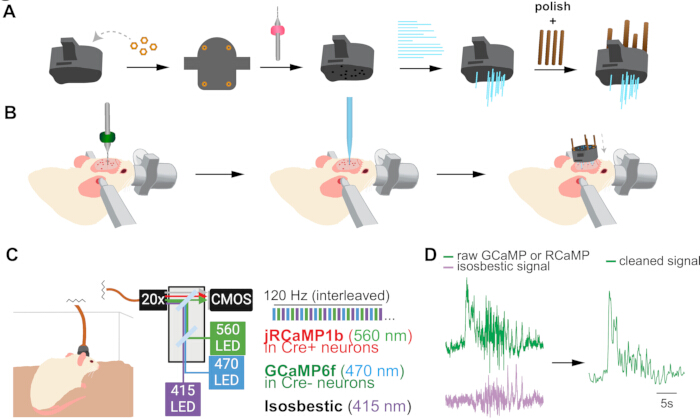
Figure 1. Recording from the Social Behavior Network using multisite, two-color fiber photometry. (A) Schematic representation of how to build a multifiber array. (B) Schematic representation of surgery workflow. (C) Schematic representation of two-color calcium imaging experiments. (D) Example of using isosbestic signal to compute a motion corrected signal. Please click here to view a larger version of this figure.

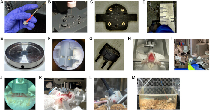
Figure 2. Images of key procedures for fabrication and surgery. (A) Fabricated patchcord ready to be used for recording. (B) Multifiber array placed into a custom stereotactic holder with the 0.25 mm x 5.5 mm drill bit positioned above a fiber through-hole. (C) Multifiber array with all fiber through-holes cleared and hex nuts glued in. (D) Cleaving a fiber using a fiber scribe. (E) Multifiber array with all fibers superglued and placed onto a custom polishing puck. (F) Magnified view of how to align and screw in the patchcord connector to the multifiber array. (G) Fully built multifiber array with dowel pins glued in place. (H) Mouse affixed to stereotactic frame with scalp incision made to expose the skull. (I) Fabricated multifiber array attached to stereotactic manipulator to maneuver the multifiber array during surgery. (J) Magnified view of the multifiber array being lowered into the brain. (K) Multifiber array fully lowered and affixed to the skull with dental cement. (L) Multifiber array on an animal that is securely connected to the patchcord prior to recording. (M) Zoomed-out view of animal in cage with patchcord connected prior to and/or during recording. Please click here to view a larger version of this figure.

Figure 3. Spectral separation. Example traces demonstrating minimal spectral crosstalk between calcium indicators. GCaMP6f (blue) signals show robust activation during 470 nm excitation but negligible response to 560 nm excitation. jRCaMP1b (red) signals exhibit the inverse pattern with strong activation from 560 nm but minimal response to 470 nm illumination. (A) Simultaneously recorded GCaMP6f and jRCaMP1b signals with 470 nm illumination only. (B) Same as (a), but with 560 nm illumination only. Please click here to view a larger version of this figure.

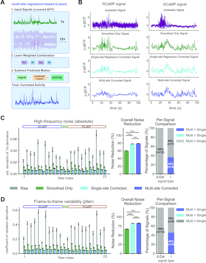
Figure 4. Comparison of Different Methods for Multifiber Signal Processing. (A) Schematic depicting multi-site regression-based correction of photometry signal. This approach involves sequential processing steps whereby all available 415nm isosbestic signals are linearly mapped to each calcium-dependent signal. Predicted motion components are subtracted from this signal to produce the final readout of activity. z-scored ΔF/F signals from two signals with strong presence of motion artifacts. (B) From top to bottom: isosbestic signal from the same fiber/imaging channel depicting motion artifacts, smoothed-only RCaMP (left) or GCaMP (right) signal (median-filtered, green), same fiber/imaging channel regression-corrected signal (cyan), multi-fiber regression-corrected signal (blue). (C) Left: Mean high-frequency noise score for each recorded signal (n = 21 sessions). High-frequency noise is computed as the standard deviation of each signal’s first derivative. Noise scores are shown for 1) baseline-corrected but uncorrected signal (gray), 2) baseline-corrected and median-filtered signal (pink), 3) baseline- and single-fiber regression-corrected signal with Savitsky-Golay smoothing (cyan), and 4) baseline- and multi-fiber regression-corrected signal with Savitsky-Golay smoothing (blue). Center: Mean percentage of noise removed using only smoothing, single-fiber or multi-fiber regression, aggregated across all 23 signals. Percentage of noise removed is calculated as the fraction of high-frequency noise resulting from correction relative to the overall level of noise in the raw, baseline-corrected signal. Data are reported as mean ± SEM (Kruskal-Wallis test, H = 501.9420, p < 0.001; post-hoc Mann-Whitney U tests with Bonferroni correction: Smoothed vs Single-site regression ***p < 0.001, Smoothed vs Multi-site regression***p < 0.001, Single-site vs Multi-site **p = 0.0073). Right: Percentage of signals whereby high-frequency noise is statistically dissimilar following single-fiber versus multi-fiber regression-based correction, separated by signal type. For each of the 23 signals, noise levels after single-site correction were compared to noise levels after multi-site correction using either independent t-tests (if normally distributed) or Mann-Whitney U tests (non-parametric alternative). Blue segments indicate signals where multi-site correction resulted in significantly lower noise than single-site correction (p < 0.05). Gray segments indicate signals with no significant difference between correction methods. Cyan segments indicate signals where single-site correction resulted in significantly lower noise. E: Vgat- GCaMP6f. DA: GRAB-DA. I: Vgat+ jRCaMP1b. (D) Same as (C) but depicting frame-to-frame variability (jitter), calculated as the derivative of the coefficient of variation of each signal (Kruskal-Wallis test, H = 495.6685, p < 0.001; post-hoc Mann-Whitney U tests with Bonferroni correction: Smoothed vs Single-site regression ***p < 0.001, Smoothed vs Multi-site regression***p < 0.001, Single-site vs Multi-site ***p = 0.0006). For complete list of statistical tests and results see Table 3. Please click here to view a larger version of this figure.

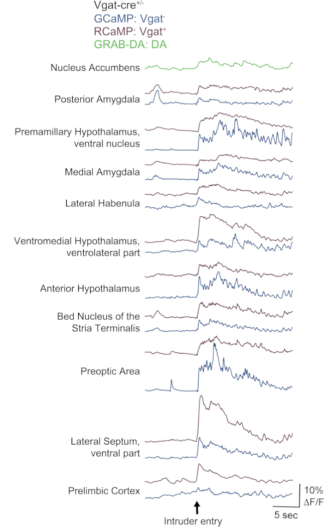
Figure 5. Multi-site showcase of dual-color fiber photometry. Representative signals from multiple indicator types recorded simultaneously during social behavior (resident-intruder test, intruder entry epoch). Traces show un-normalized and baseline-subtracted but not motion-artifact-corrected GCaMP6f (Cre-negative neurons), jRCaMP1b (GABAergic Vgat-Cre+ neurons), and GRAB-DA1m (dopamine sensor in nucleus accumbens) across social behavior network sites in the same animal. Please click here to view a larger version of this figure.

Table 1. Virus Coordinates and Fiber Lengths for each targeted Social Behavior Network Brain Region. Please click here to download this Table.

Table 2. Comparison of Motion Artifact Correction Methods for Multi-Site Fiber Photometry. Underlying principles, optimal use cases, advantages and limitations of the following motion artifact correction methods: simple linear regression, Lasso regression with L1 regularization (using multi-predictor approach), Bayesian generative modeling, frequency-based scaling, and iteratively reweighted least squares. Please click here to download this Table.

Table 3. Details and results of the statistical tests used in Figure 4. Please click here to download this Table.

Supplemental File 1. 3D print file for patchcord connector.Please click here to download this file.

Supplemental File 2. 3D print file for patchcord connector without through holes.Please click here to download this file.

Supplemental File 3. 3D print file for stereotactic drilling accessory.Please click here to download this file.

Supplemental File 4. Custom polishing puck blueprint.Please click here to download this file.

Supplemental File 5. 3D print file for multisite photometry array targeting 12 SBN sites.Please click here to download this file.

Supplemental File 6. 3D print file for multisite photometry array without through holes targeting sites.Please click here to download this file.

Supplemental File 7. DAQ configuration file for DAQ software.Please click here to download this file.

Supplemental File 8. Visual coding file for photometry system.Please click here to download this file.

Supplemental File 9. Python code used in Protocol Step 4 and for motion artifact corrected comparisons. Please click here to download this file.

Discussion

Fiber photometry is a useful and cost effective technique for recording population calcium activity from deep brain regions or specific cell types in the freely moving animal³. Recording from multiple brain regions simultaneously allows the user to compare the dynamics across regions or projections during naturalistic behavior or head-fixed preparations^5,7,12. Here, we detail methods to record in two colors from up to 12 brain regions across the brain’s subcortical “social behavior network” using a bespoke fiber array and a commercially available camera system. Below, we discuss critical steps in implementing this method, potential modifications and troubleshooting strategies, and its significance as well as limitations relative to existing approaches.

The protocol involves three major phases. First, multifiber array and patchcord fabrication requires custom 3D-printed parts to be drilled at stereotactic coordinates, followed by fiber insertion, polishing, and quality control to ensure ≥75% light transmission efficiency. Precise drilling alignment (±0.03 mm tolerance) and thorough polishing are critical. Common failures include low light transmission efficiency (<75%) and blocked fiber through-holes. Low efficiency typically results from fiber blemishes during cleaving or improper polishing. Solutions include verifying each fiber end is unblemished under brightfield microscopy before insertion (step 1.1.6.2), re-polishing using the complete grit progression (6 µm → 0.01 µm, step 1.1.6.1), and ensuring the fiber cleaver blade is sharp. To improve throughput, laboratories can implement workflow modifications such as custom fiber cutting jigs using precision translation stages or laser-based cutting systems (step 1.2.4). Commercial 3D printing manufacturers with high-precision systems can reduce manual drilling needs (steps 1.1.3–1.1.4, step 1.2.3), though dimensional accuracy may vary between batches.

Second, surgical implantation involves skull leveling (±0.03 mm tolerance), viral injections at 11–12 sites, and multifiber array implantation followed by cement fixation. Targeting accuracy is compromised when skull leveling exceeds tolerance. This can be mitigated by measuring pitch at multiple anterior-posterior points 8.25 mm apart and measuring roll at ±2.0–2.5 mm lateral positions, while ensuring ear bars fully stabilize the skull. Air bubbles in virus injection micropipettes prevent accurate delivery and necessitate restarting micropipette preparation (step 2.9). During multifiber array implantation, avoid cement contact with fiber tips by building cement pyramids from the skull surface upward (steps 2.10.3–2.10.5) and allow adequate drying time (≥15 min).

Third, recording and data processing involves camera synchronization via a DAQ system, LED power calibration (0.1 mW output/fiber, 1.2 mW output/12-fiber patchcord), and signal preprocessing with isosbestic controls. The motion correction pipeline introduced here uses Lasso regression, which is well-suited for multi-channel predictor configurations because it automatically shrinks uninformative predictors toward zero, retaining only those that meaningfully contribute to artifact correction. This property makes it particularly advantageous for dual-color photometry: by including isosbestic signals from both red and green channels as predictors, Lasso selectively leverages whichever channels carry genuine motion information, yielding substantially better noise reduction in red channel (RCaMP) signals compared to same-fiber correction alone (Figure 4C–D). Because Lasso identifies the most informative predictors automatically, using all available isosbestic channels as input is strongly recommended. That said, Lasso regression is one of several valid correction methods; alternatives include Bayesian generative modeling⁴⁶, frequency-based scaling⁴⁷, and iteratively reweighted least squares (IRLS)⁴⁸, all of which likely yield comparable artifact reduction, with implementation guidance provided in Table 2. Persistent poor signal quality despite optimized preprocessing likely indicates hardware or surgical issues, and steps 1–2 should be revisited

Beyond these procedural considerations, dual-color photometry introduces additional technical challenges related to spectral separation. A critical consideration in dual-color photometry is managing spectral overlap between green and red calcium indicators. While complete elimination of spectral crosstalk is challenging due to overlapping emission spectra of GCaMP and RCaMP, our temporal multiplexing approach with interleaved LED excitation (470 nm for GCaMP, 560 nm for RCaMP, 415 nm isosbestic) and optimized bandpass emission filters substantially mitigates this issue. In practice, we observe minimal crosstalk: 470 nm stimulation evokes negligible activity in the red channel, and vice versa for 560 nm stimulation in the green channel (Figure 3). Researchers concerned about residual spectral overlap can further optimize their systems by selecting narrow-bandpass emission filters with maximal spectral separation based on their specific indicator combinations.

Compared to other approaches for large-scale neural recordings, bespoke two-color multisite fiber photometry offers many significant advantages. First, while single fiber photometry^1,2,3, contemporary extracellular recordings^4,6, or cortical surface imaging approaches^8,9 are restricted to a single or a spatially constrained set of brain regions (e.g., at the cortical surface), the customizable 3D print design we share here permits the targeting of up to 12 brain regions anywhere in the brain with 200 µm optical fibers. In comparison, commercially available multifiber ferrules^5,7 only support 100 µm fiber optics and are similarly constrained to a limited set of brain regions directly ventral to the linear array of the ferrule. With regards to targeting and recording from specific brain regions, the primary trade-off is between fiber diameter and the photometry system's field of view. The 3D printed multifiber arrays equipped with 200 µm fibers record from a larger area at each site compared to commercially available multifiber ferrules. In the current protocol, the photometry system’s camera field of view limits recording to 12 optic fibers at 200 µm. This constraint can be overcome by reducing fiber diameter to 100 µm for up to 60 fibers or by building a custom photometry system with a larger camera objective.

Finally, this customizable, two-color multisite fiber photometry platform has been used to longitudinally track neural activity dynamics of two genetically distinct neural populations across 11-12 brain regions. Using a Cre-in/Cre-excluding strategy expressing Cre-dependent RCaMP and Cre-excluding GCaMP across SBN populations in a Vgat-cre mouse, both aggressive experience and observation were shown to promote shared patterns of SBN-wide activity dynamics during future defensive social interactions⁴². Using the same viral strategy in an Esr1-cre mouse to record from estrogen receptor alpha expressing and non-expressing neurons, territory-specific patterns of social behavior were associated with rapid, hormone-sensitive rescaling of an SBN-wide social action code, boosting behavior-associated activity in the home territory⁴³. These territory-specific differences in behavior and network encoding require circulating testosterone in male mice. While these studies used a viral approach and a single Cre line, future studies can expand these methods with intersectional viral approaches, genetically expressed calcium indicators, or fluorescent reporters of neuromodulator and neuropeptide signaling.

Materials

List of materials used in this article

Name	Company	Catalog Number	Comments
#76 drill bit	Drill Bit City	#76
#78 drill bit	Drill Bit City	#78
#92 drill bit	Drill Bit City	#92
0.01 μm grit polishing sheets	ThorLabs	LFCF2
0.25 mm x 5.5 mm drill bits	Drill Bit City	custom product	0.25 x 5.5 mm drill bit , contacted company to build
1 μm grit polishing sheets	ThorLabs	LF1D
12 fiber-branching patchord	Doric Lens	CustomBBP(12)_200/220/3000-0.37 _5m_SMA-12xCL_LAF
200 μm optic fiber	ThorLabs	FT200UMT
3 μm grit polishing sheets	ThorLabs	LF3D
30 μm grit polishing sheets	ThorLabs	LF30D
6 μm grit polishing sheets	ThorLabs	LF6D
Absorbable suture	Ethicon	J421H
Adaptive Iteratively Reweighted Penalized Least Squares documentation	Google	N/A	https://code.google.com/archive/p/airpls/
Alloy steel dowel pins	McMaster-Carr	98381a983
Behavior cameras	Teledyne FLIR	Blackfly S
Bonsai	Bonsai Software Foundation	version 2.9.0
Brightfield Microscope	Leica	ES2
Bulldog clamps	FineScienceTools	18038-45
DAQ	Measurement Computing	MC USB-200 series DAQ
DAQ software	Measurement Computing	DAQami
Drill	Kopf Instruments	Model 1911 Stereotaxic Drill
Fiber cleaver	ThorLabs	XL411/CLVB
Fiber photometry system	Neurophotometrics	FP3002
Fiber photometry system manual	Neurophotometrics	N/A	Webpage hosting device manual: https://neurophotometrics.com/documentation
Fiber scribe	ThorLabs	S90C
Fiber stripper	ThorLabs	T10S13
Fine forceps	FineScienceTools	11252-00
Fine scissors	FineScienceTools	14084-08
G5 drive screws	Open Ephys Production Site	OEPS-7105
G5 screwdriver	Open Ephys Production Site	OEPS-7121
GCaMP6f	PNI Viral Neuroengineering Lab	EF1a-Cre out-GCaMP6f-WPRE-hGHpA
GRAB-DA	Addgene	hSyn-GRAB_DA1m-WPRE-hGHpA
Heating pad	Adroit Medical Supplies	HTP-1500
Heating system	Kent Scientific	RT-0515
Isoflurane	Covetrus	29405
jRCaMP1b	Addgene	pAAV.Syn.Flex.NES-jRCaMP1b.WPRE.SV40
M0.6 Brass hex nuts	MetricScrews.us	21614
Metabond cement reagents and tools	Parkell	S380
MicroFine ABS-like resin 3D prints	ProtoLabs	custom product	See Supplemental Code Files 1-3, 5, 6
Nanoliter injector	Drummond Scientific Company	Nanoject II	nanoliter injector
Parrafin wax sheets	Amcor	ParaFilm M All-Purpose Laboratory Film
Pipetter	ThermoFisher Scientific	4641310N
Polishing Puck	Princeton University Physics Department Machine Shop	custom product	See Supplemental Code File 4
Powermeter	ThorLabs	PM100D
Puralube optical ointment	Dechra	P1490-1
Python	Python Software Foundation	N/A
Soft plastic tubing for patchcord	McMaster-Carr	3774N4
SpinView	Teledyne FLIR	version 1.25.0.52	Imaging software that controls the behavior cameras
Stereotactic frame	Kopf Instruments	Model 1900
TMAC documentation	N/A	N/A	TMAC code: https://github.com/Nondairy-Creamer/tmac
Tubing for stereotactic frame	Saint-Gobain	E-3603
Vaporizer	Kent Scientific	VetFlo Vaporizer

References

- Cui, G., et al. Concurrent activation of striatal direct and indirect pathways during action initiation. Nature. 494 (7436), 238-242 (2013).
- Adelsberger, H., Zainos, A., Alvarez, M., Romo, R., Konnerth, A. Local domains of motor cortical activity revealed by fiber-optic calcium recordings in behaving nonhuman primates. Proceedings of the National Academy of Sciences. 111 (1), 463-468 (2014).
- Gunaydin, L. A., et al. Natural Neural Projection Dynamics Underlying Social Behavior. Cell. 157 (7), 1535-1551 (2014).
- Jun, J. J., et al. Fully integrated silicon probes for high-density recording of neural activity. Nature. 551 (7679), 232-236 (2017).
- Sych, Y., Chernysheva, M., Sumanovski, L. T., Helmchen, F. High-density multi-fiber photometry for studying large-scale brain circuit dynamics. Nature Methods. 16 (6), 553-560 (2019).
- Steinmetz, N. A., et al. Neuropixels 2.0: A miniaturized high-density probe for stable, long-term brain recordings. Science. 372 (6539), (2021).
- Guo, Z., et al. Neural dynamics in the limbic system during male social behaviors. Neuron. 111 (20), 3288-3306.e4 (2023).
- Ma, Y., et al. Wide-field optical mapping of neural activity and brain haemodynamics: considerations and novel approaches. Philosophical Transactions of the Royal Society B: Biological Sciences. 371 (1705), 20150360(2016).
- Musall, S., Kaufman, M. T., Juavinett, A. L., Gluf, S., Churchland, A. K. Single-trial neural dynamics are dominated by richly varied movements. Nature Neuroscience. 22 (10), 1677-1686 (2019).
- Zhou, Z. C., et al. Deep-brain optical recording of neural dynamics during behavior. Neuron. 111 (23), 3716-3738 (2023).
- Martianova, E., Aronson, S., Proulx, C. D. Multi-Fiber Photometry to Record Neural Activity in Freely-Moving Animals. JoVE. (152), e60278(2019).
- Kim, C. K., et al. Simultaneous fast measurement of circuit dynamics at multiple sites across the mammalian brain. Nature Methods. 13 (4), 325-328 (2016).
- Newman, S. W. The Medial Extended Amygdala in Male Reproductive Behavior A Node in the Mammalian Social Behavior Network. Annals of the New York Academy of Sciences. 877, 242-257 (1999).
- Goodson, J. L. The vertebrate social behavior network: Evolutionary themes and variations. Hormones and Behavior. 48 (1), 11-22 (2005).
- O’Connell, L. A., Hofmann, H. A. Evolution of a Vertebrate Social Decision-Making Network. Science. 336 (6085), 1154-1157 (2012).
- Wu, M. V., Tollkuhn, J. Estrogen receptor alpha is required in GABAergic, but not glutamatergic, neurons to masculinize behavior. Hormones and Behavior. 95, 3-12 (2017).
- Moffitt, J. R., et al. spatial, and functional single-cell profiling of the hypothalamic preoptic region. Science. 362 (6416), eaau5324(2018).
- Gegenhuber, B., Wu, M. V., Bronstein, R., Tollkuhn, J. Gene regulation by gonadal hormone receptors underlies brain sex differences. Nature. 606 (7912), 153-159 (2022).
- Knoedler, J. R., et al. A functional cellular framework for sex and estrous cycle-dependent gene expression and behavior. Cell. 185 (4), 654-671.e22 (2022).
- Musatov, S., Chen, W., Pfaff, D. W., Kaplitt, M. G., Ogawa, S. RNAi-mediated silencing of estrogen receptor in the ventromedial nucleus of hypothalamus abolishes female sexual behaviors. Proceedings of the National Academy of Sciences. 103 (27), 10456-10460 (2006).
- Lee, H., et al. Scalable control of mounting and attack by Esr1+ neurons in the ventromedial hypothalamus. Nature. 509 (7502), 627-632 (2014).
- Hashikawa, K., et al. Esr1+ cells in the ventromedial hypothalamus control female aggression. Nature Neuroscience. 20 (11), 1580-1590 (2017).
- Fang, Y. -Y., Yamaguchi, T., Song, S. C., Tritsch, N. X., Lin, D. A Hypothalamic Midbrain Pathway Essential for Driving Maternal Behaviors. Neuron. 98 (1), 192-207.e10 (2018).
- Wei, Y. -C., et al. Medial preoptic area in mice is capable of mediating sexually dimorphic behaviors regardless of gender. Nature Communications. 9 (1), 279(2018).
- Yamaguchi, T., Wei, D., Song, S. C., Lim, B., Tritsch, N. X., Lin, D. Posterior amygdala regulates sexual and aggressive behaviors in male mice. Nature Neuroscience. 23 (9), 1111-1124 (2020).
- Yang, B., Karigo, T., Anderson, D. J. Transformations of neural representations in a social behaviour network. Nature. , (2022).
- Jacobowitz, D. M., O’Donohue, T. L. alpha-Melanocyte stimulating hormone: immunohistochemical identification and mapping in neurons of rat brain. Proceedings of the National Academy of Sciences. 75 (12), 6300-6304 (1978).
- Flanigan, M. E., et al. Orexin signaling in GABAergic lateral habenula neurons modulates aggressive behavior in male mice. Nature Neuroscience. 23 (5), 638-650 (2020).
- Bayless, D. W., et al. A neural circuit for male sexual behavior and reward. Cell. 186 (18), 3862-3881.e28 (2023).
- Dawson, M., et al. Hypocretin/orexin neurons encode social discrimination and exhibit a sex-dependent necessity for social interaction. Cell Reports. 42 (7), 112815(2023).
- Iyilikci, O., et al. Age-specific regulation of sociability by hypothalamic Agrp neurons. bioRxiv. , (2025).
- Patriarchi, T., et al. Ultrafast neuronal imaging of dopamine dynamics with designed genetically encoded sensors. Science. 360 (6396), eaat4422(2018).
- Sun, F., et al. A Genetically Encoded Fluorescent Sensor Enables Rapid and Specific Detection of Dopamine in Flies, Fish, and Mice. Cell. 174 (2), 481-496.e19 (2018).
- Sun, F., et al. Next-generation GRAB sensors for monitoring dopaminergic activity in vivo. Nature Methods. 17 (11), 1156-1166 (2020).
- Duffet, L., et al. A genetically encoded sensor for in vivo imaging of orexin neuropeptides. Nature Methods. 19 (2), 231-241 (2022).
- Ino, D., Tanaka, Y., Hibino, H., Nishiyama, M. A fluorescent sensor for real-time measurement of extracellular oxytocin dynamics in the brain. Nature Methods. 19 (10), 1286-1294 (2022).
- Wang, H., et al. A tool kit of highly selective and sensitive genetically encoded neuropeptide sensors. Science. 382 (6672), eabq8173(2023).
- Dong, C., et al. Unlocking opioid neuropeptide dynamics with genetically encoded biosensors. Nature Neuroscience. 27 (9), 1844-1857 (2024).
- Chen, T. -W., et al. Ultrasensitive fluorescent proteins for imaging neuronal activity. Nature. 499 (7458), 295-300 (2013).
- Dana, H., et al. Sensitive red protein calcium indicators for imaging neural activity. eLife. 5, e12727(2016).
- Zhang, Z. -M., Chen, S., Liang, Y. -Z. Baseline correction using adaptive iteratively reweighted penalized least squares. The Analyst. 135 (5), 1138(2010).
- Iravedra-Garcia, J. M., Guthman, E. M., Cuturela, L., Ocasio-Arce, E. J., Pillow, J. W., Falkner, A. L. Aggression experience and observation promote shared behavioral and neural changes. bioRxiv. , (2024).
- Guthman, E. M., Iravedra-Garcia, J. M., Sirrs, L., Le, A., Falkner, A. L. Context rescales a social action code in a hormone-sensitive network. bioRxiv. , (2025).
- Saunders, A., Johnson, C. A., Sabatini, B. L. Novel recombinant adeno-associated viruses for Cre activated and inactivated transgene expression in neurons. Frontiers in Neural Circuits. 6, (2012).
- Creamer, M. S., Chen, K. S., Leifer, A. M., Pillow, J. W. Correcting motion induced fluorescence artifacts in two-channel neural imaging. PLOS Computational Biology. 18 (9), e1010421(2022).
- Donka, R. M., Loh, M. K., Konanur, V. R., Roitman, M. F., Roitman, J. D. PASTa: An Open-Source Analysis and Signal Processing Toolbox for Fiber Photometry Data. Current Protocols. 5 (7), e70161(2025).
- Keevers, L. J., Jean-Richard-dit-Bressel, P. Obtaining artifact-corrected signals in fiber photometry via isosbestic signals, robust regression, and dF/F calculations. Neurophotonics. 12 (02), (2025).