This protocol describes a reproducible two-sample Mendelian randomization workflow for evaluating the potential causal association between ischemic stroke and vascular dementia using publicly available genome-wide association study summary statistics.
Method Article
Causal Relationship Between Ischemic Stroke and Vascular Dementia: A Mendelian Randomization Study
58 views
⸱
September 11th, 2026
In This Article
Summary
Abstract
Ischemic stroke (IS) is a major cause of disability and mortality worldwide, and vascular dementia (VaD) is a common dementia subtype associated with cerebrovascular injury. Observational studies have suggested a relationship between IS and VaD, but these studies are vulnerable to confounding and reverse causality. This protocol describes a reproducible two-sample Mendelian randomization (MR) workflow for evaluating the potential causal association between IS and VaD using publicly available genome-wide association study (GWAS) summary statistics. Genetic instruments associated with IS were extracted from a public GWAS dataset, and outcome associations for VaD were obtained from a public VaD GWAS dataset. The corresponding dataset IDs are provided in the Protocol section. After outcome matching and allele harmonization, 51 single-nucleotide polymorphisms (SNPs) were retained for the final MR analysis. The workflow includes instrumental variable selection, linkage disequilibrium clumping, allele harmonization, instrument strength assessment, inverse variance weighted (IVW) analysis, weighted median analysis, MR-Egger analysis, heterogeneity testing, horizontal pleiotropy assessment, and leave-one-out sensitivity analysis. In the representative analysis, the IVW method showed a positive association between genetically predicted IS and VaD risk, and the weighted median method yielded a directionally concordant result. The MR-Egger estimate was directionally consistent but did not reach statistical significance. Therefore, these findings should be interpreted as suggestive evidence of a possible causal effect, rather than definitive proof of causality. This protocol may help researchers apply a transparent and reproducible MR workflow to investigate cerebrovascular disease-related outcomes using public GWAS data.
Introduction
Ischemic stroke (IS) is a leading cause of severe disability and death worldwide1. According to the latest data from the Global Burden of Disease Study, the global incidence of IS has declined, but it remains a significant burden, especially in Eastern Europe, East Asia, Central Asia, and Sub-Saharan Africa2,3. Furthermore, the incidence of IS is on the rise in countries with a low Socio-demographic Index (SDI), and it is projected to continue increasing from 2020 to 2030.
Numerous epidemiological studies have suggested a potential link between cerebrovascular diseases and vascular dementia (VaD)4,5. Particularly in China, VaD is one of the most common types of dementia among the elderly, and the high prevalence of IS is closely associated with the onset of VaD. However, most existing studies are observational, and residual confounding, reverse causality, and differences in disease definition may limit causal interpretation. Therefore, additional analytical approaches are needed to evaluate whether IS is potentially involved in the development of VaD.
IS may influence the onset of VaD through several mechanisms. Cerebrovascular damage caused by IS can lead to insufficient cerebral perfusion and subsequent neurodegenerative changes6. In addition, VaD may be related to chronic cerebrovascular injury, microvascular damage, and inflammatory responses after IS7,8. Therefore, investigating the relationship between IS and VaD is important for understanding potential disease links and guiding future prevention strategies.
Mendelian randomization (MR) is an analytical method that uses genetic variants as instrumental variables to evaluate potential causal associations between an exposure and an outcome9. Compared with conventional observational studies, MR can reduce confounding and reverse causality bias under valid instrumental variable assumptions. Compared with randomized controlled trials or experimental models, MR can use existing genome-wide association study (GWAS) summary statistics to evaluate clinically relevant associations when direct intervention studies are infeasible, unethical, or difficult to conduct. Recent genetic studies using Mendelian-randomization approaches have investigated the association between IS and VaD10. However, detailed protocol-level descriptions of exposure instrument selection, outcome data extraction, allele harmonization, instrument strength assessment, heterogeneity testing, pleiotropy assessment, and sensitivity analyses remain important for reproducible implementation.
This protocol is appropriate when publicly available GWAS summary statistics are available for both the exposure and outcome of interest, valid genetic instruments can be selected for the exposure, and the research question aims to evaluate a potential causal association rather than directly establish biological mechanisms. This study therefore presents a two-sample MR protocol for evaluating the potential causal association between IS and VaD using publicly available GWAS summary statistics. The aim is to provide a reproducible analytical workflow rather than to establish definitive biological mechanisms. This protocol describes genetic instrument selection, outcome matching, allele harmonization, MR estimation, and sensitivity analyses, and uses the IS-VaD association as a representative example.
Protocol
This study used publicly available GWAS summary statistics. The original studies had obtained institutional review board approval and informed consent from participants. No additional ethical approval was required for this secondary analysis.
1. Study design and ethics statement
- Use a two-sample MR design to evaluate the potential causal association between IS and VaD.
- Use only publicly available GWAS summary statistics. Because all original studies included in the GWAS datasets had obtained institutional review board approval and informed consent from participants, no additional ethical approval is required for this secondary analysis.
- Define IS as the exposure and VaD as the outcome before data extraction.
2. Software preparation
- Conduct all analyses using R statistical software.
- Load the TwoSampleMR package for instrument extraction, outcome data extraction, allele harmonization, MR estimation, heterogeneity testing, and sensitivity analyses. Load the MRPRESSO package to assess global horizontal pleiotropy and potential outlier variants.
- Use the following core functions in the workflow: extract_instruments, extract_outcome_data, harmonise_data, mr, generate_odds_ratios, mr_heterogeneity, mr_pleiotropy_test, mr_singlesnp, mr_leaveoneout, mr_scatter_plot, mr_forest_plot, mr_funnel_plot, and mr_leaveoneout_plot. Use MRPRESSO::mr_presso to perform the MR-PRESSO global test and, when applicable, outlier and distortion tests.
3. Exposure dataset selection and instrumental variable screening
- Extract IS-associated single-nucleotide polymorphisms (SNPs) from the IEU OpenGWAS dataset ebi-a-GCST90018864. This dataset includes 11,929 IS cases and 472,192 controls, with a total sample size of 484,121 participants.
- Select candidate SNPs associated with IS using a significance threshold of p < 5 × 10⁻⁶.
- The p < 5 × 10⁻⁶ threshold is used in this representative protocol to retain an adequate number of independent instruments for sensitivity analyses. Because this threshold is less stringent than the conventional genome-wide significance threshold, findings based on these instruments should be interpreted as exploratory and suggestive rather than definitive.
- Perform linkage disequilibrium clumping to retain independent SNPs. Use an r2 threshold of 0.001 and a clumping window of 10,000 kb.
- Use the following R command to extract candidate instruments:
extract_instruments(outcomes = "ebi-a-GCST90018864", p1 = 5e-06, clump = TRUE) - Calculate the F-statistic for each retained SNP using the formula F = (β/SE)2, where β and SE are the SNP–exposure effect estimate and standard error, respectively.
- Exclude SNPs with an F-statistic < 10 to reduce the risk of weak instrument bias. Summarize the distribution of F-statistics using the minimum, maximum, median, and interquartile range (IQR).
4. Outcome dataset extraction
- Extract VaD outcome associations from the FinnGen GWAS dataset finn-b-F5_VASCDEM. This dataset includes 881 VaD cases and 211,508 controls.
- Extract the outcome associations for all selected IS-associated SNPs using the extract_outcome_data function.
- Search for proxy SNPs when target SNPs are not directly available in the outcome dataset. Retain proxy-matched variants when valid proxy information and allele correspondence are available.
- Use the following R command to extract the outcome dataset:
extract_outcome_data(snps = exp_dat$SNP, outcomes = "finn-b-F5_VASCDEM", access_token = NULL)
5. Allele harmonization and SNP retention
- Harmonize the exposure and outcome datasets before MR analysis.
- Align the effect allele and other allele so that the SNP–exposure and SNP–outcome effect estimates correspond to the same effect allele.
- Inspect SNPs during harmonization to identify allele mismatches, unavailable outcome associations, and ambiguous allele alignment. Retain SNPs with available exposure and outcome effect estimates after harmonization.
- Use the following R command for allele harmonization: harmonise_data(exposure_dat = exp_dat, outcome_dat = out_dat, action = 1)
- Record the number of SNPs initially extracted from the exposure dataset, the number of SNPs with available outcome associations, the number of proxy-matched variants, and the number of SNPs retained for the final MR analysis.
6. Primary MR analysis and sensitivity analyses
- Perform the primary MR analysis using the inverse variance weighted (IVW) method.
- Perform complementary MR analyses using the weighted median and MR-Egger methods to assess the consistency of the causal estimate under different assumptions.
- Generate odds ratios (ORs) and 95% confidence intervals (CIs) from the MR estimates.
- Use the following R commands to run the MR analysis and calculate ORs:
res <- mr(dat)
res <- generate_odds_ratios(res) - Because one prespecified primary exposure–outcome association is evaluated, define the Bonferroni-corrected threshold for the primary MR inference as 0.05/1 = 0.05. Use a two-sided p-value < 0.05 as the statistical significance threshold for the primary IVW analysis.
- To contextualize the statistical precision of the primary analysis given the limited number of VaD cases, perform a post hoc two-sided Wald-test power calculation based on the observed IVW estimate and its standard error. Calculate the power using the non-centrality parameter βIVW/SEIVW at a two-sided α level of 0.05. Calculate the minimum detectable effect corresponding to 80% power as exp[(z0.975 + z0.80) × SE]. Because IS is a binary exposure and SNP–exposure associations are expressed on the log-odds scale, report this analysis as an effect-conditioned descriptive assessment of precision rather than as a prespecified sample-size calculation11.
7. Heterogeneity, horizontal pleiotropy, and leave-one-out analyses
- Assess between-SNP heterogeneity using Cochran’s Q statistic.
- Use the following R command to calculate heterogeneity statistics:
mr_heterogeneity(dat) - Assess directional horizontal pleiotropy using the MR-Egger intercept test.
- Use the following R command to calculate the MR-Egger intercept:
mr_pleiotropy_test(dat) - Assess global horizontal pleiotropy and potential outlier variants using MR-PRESSO with 10,000 simulations, a significance threshold of 0.05, and both outlier and distortion tests enabled12.
- Use the following R command for MR-PRESSO analysis:
set.seed(20260729)
mr_presso(
BetaOutcome = "beta.outcome",
BetaExposure = "beta.exposure",
SdOutcome = "se.outcome",
SdExposure = "se.exposure",
OUTLIERtest = TRUE,
DISTORTIONtest = TRUE,
data = dat,
NbDistribution = 10000,
SignifThreshold = 0.05
) - Perform single-SNP analysis to estimate the effect of each SNP separately.
- Use the following R command for single-SNP analysis:
res_single <- mr_singlesnp(dat) - Perform leave-one-out analysis by sequentially removing one SNP at a time and repeating the IVW analysis.
- Use the following R command for leave-one-out analysis:
res_loo <- mr_leaveoneout(dat)
8. Visualization and output
- Generate a scatter plot to show the MR estimates across different methods.
- Generate a forest plot to show the single-SNP estimates and the overall MR estimate.
- Generate a funnel plot to visually assess the symmetry of SNP-specific estimates.
- Generate a leave-one-out plot to assess whether the overall estimate is driven by a single SNP.
- Use the following R commands to generate the plots:
mr_scatter_plot(res, dat)
mr_forest_plot(res_single)
mr_funnel_plot(res_single)
mr_leaveoneout_plot(res_loo) - Export the MR results, instrumental variable table, outcome association table, and sensitivity analysis outputs for reporting and reproducibility.
Results
Figure 1 summarizes the overall workflow of the two-sample Mendelian randomization protocol, from dataset selection and instrument screening through sensitivity analyses and result visualization. Representative outputs from each stage are presented below.
Genetic instrumental variables and harmonization quality control
A total of 52 IS-associated SNPs were initially extracted from the exposure GWAS dataset using a significance threshold of p < 5 × 10⁻⁶. Outcome associations were then extracted from the VaD GWAS dataset. After outcome matching, proxy searching, and allele harmonization, 51 SNPs were retained for the final MR analysis. Two variants were matched using proxy SNPs. The retained genetic instruments are listed in Table 1. The F-statistics of the 51 retained instruments ranged from 20.91 to 46.06, with a median of 25.08 and an IQR of 22.95–30.71. No retained SNP had an F-statistic below 10, indicating a low likelihood of weak instrument bias.
MR estimates for IS and VaD
The scatter plot showed the direction and magnitude of the SNP-specific MR estimates across different MR methods (Figure 2). The IVW and weighted median methods showed positive associations, whereas the MR-Egger estimate was directionally consistent but did not reach statistical significance.
The forest plot of individual SNP estimates showed the SNP-specific associations with VaD risk (Figure 3). The overall MR estimates are summarized in Figure 4. The IVW method showed a statistically significant positive association between genetically predicted IS and VaD risk (OR = 1.63, 95% CI: 1.21–2.21, p = 0.0013). The weighted median method yielded a concordant significant estimate (OR = 1.60, 95% CI: 1.06–2.42, p = 0.0240). The MR-Egger estimate was directionally consistent but did not reach statistical significance (OR = 2.21, 95% CI: 0.97–5.01, p = 0.0645).
The FinnGen VaD outcome GWAS included 881 cases and 211,508 controls. In a post hoc two-sided Wald-test calculation conditional on the observed IVW estimate, the estimated power for the primary IVW analysis was 89.5% at α = 0.05. The corresponding minimum detectable effect for 80% power was an OR of 1.54. In contrast, the minimum detectable effect for the MR-Egger analysis was an OR of 3.23, which exceeded the observed directionally consistent MR-Egger estimate (OR = 2.21). Therefore, the non-significant MR-Egger result should be interpreted as reflecting the limited precision of this less efficient sensitivity estimator rather than, by itself, evidence against the direction of the primary IVW estimate.
Because one prespecified primary exposure–outcome association was evaluated, the Bonferroni-corrected threshold for the primary MR inference was 0.05/1 = 0.05. Therefore, the IVW result met the corrected significance threshold. Taken together, these findings provide suggestive evidence of a possible positive effect of genetically predicted IS on VaD risk, primarily based on the IVW estimate and supported by the weighted median sensitivity analysis. However, the MR-Egger estimate was directionally consistent but did not reach statistical significance; therefore, the results should not be interpreted as definitive evidence of causality.
Heterogeneity and horizontal pleiotropy analyses
Between-SNP heterogeneity was assessed using Cochran’s Q statistic. The IVW heterogeneity test yielded Q = 57.46 with 50 degrees of freedom (p = 0.218), and the MR-Egger heterogeneity test yielded Q = 56.77 with 49 degrees of freedom (p = 0.208). These results did not indicate substantial heterogeneity across SNP-specific estimates. Directional horizontal pleiotropy was assessed using the MR-Egger intercept test. The MR-Egger intercept was -0.0195 (SE = 0.0253, p = 0.444), indicating no statistical evidence of directional horizontal pleiotropy. MR-PRESSO analysis was conducted using the 51 retained harmonized SNPs with 10,000 simulations. The MR-PRESSO global test showed no evidence of global horizontal pleiotropy (RSSobs = 59.61; empirical p = 0.2388). Because the global test was not statistically significant, the individual outlier and distortion tests were not applicable, and no outlier-corrected estimate was generated. The funnel plot provided a visual assessment of the symmetry of SNP-specific estimates (Figure 5). Detailed MR-PRESSO settings and results are reported in Supplementary Table 1.
Leave-one-out sensitivity analysis and protocol output validation
Leave-one-out analysis was performed to evaluate whether the overall MR estimate was driven by any single SNP. The leave-one-out plot showed that sequential removal of individual SNPs did not materially change the overall estimate (Figure 6), suggesting that no single genetic instrument dominated the association. Together, these representative results demonstrate the practical output of the two-sample MR workflow described in this protocol. Table 1 shows the retained genetic instruments after SNP selection and harmonization. Figure 2 illustrates the direction of MR estimates across methods, Figure 3 presents SNP-specific estimates, Figure 4 summarizes the overall MR estimates, Figure 5 supports visual assessment of pleiotropy or asymmetry, and Figure 6 evaluates the influence of individual SNPs. Supplementary Table 2 links each major protocol step to its corresponding validating output.
All raw GWAS summary statistics analyzed in this study are publicly available. The ischemic stroke exposure dataset was obtained from the IEU OpenGWAS database under dataset ID ebi-a-GCST90018864. The vascular dementia outcome dataset was obtained from the FinnGen GWAS dataset under dataset ID finn-b-F5_VASCDEM. The extracted instrumental variable table, harmonized analysis dataset, MR result tables, and relevant output files are provided as supplementary files.
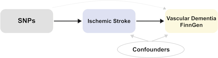
Figure 1. Workflow of the two-sample MR protocol. This figure summarizes the main steps of the protocol, including exposure dataset selection, instrumental variable screening, outcome data extraction, allele harmonization, MR estimation, heterogeneity testing, horizontal pleiotropy assessment, leave-one-out analysis, and visualization. Please click here to view a larger version of this figure.
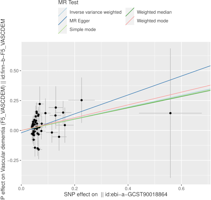
Figure 2. Scatter plot of MR estimates for the association between IS and VaD. Each point represents an SNP-specific estimate. The fitted lines represent the estimated association obtained using different MR methods. Please click here to view a larger version of this figure.
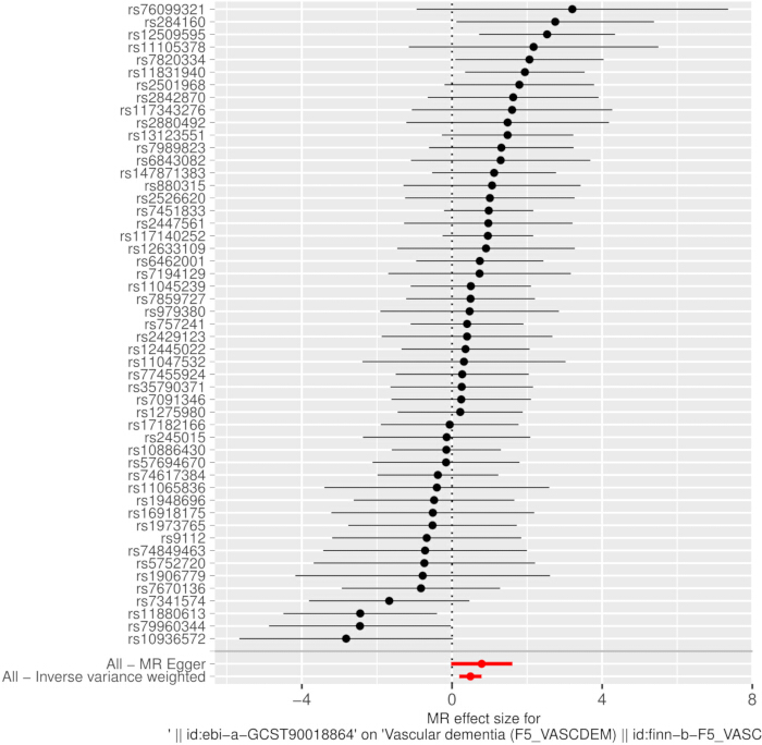
Figure 3. Forest plot of single-SNP MR estimates. This figure shows the individual SNP-specific estimates for the association between IS-associated genetic variants and VaD risk. Horizontal lines represent 95% confidence intervals. Please click here to view a larger version of this figure.
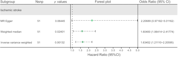
Figure 4. Forest plot of overall MR estimates across different methods. This figure summarizes the overall MR estimates obtained using the IVW, weighted median, and MR-Egger methods. Horizontal lines represent 95% confidence intervals. MR, Mendelian randomization; IVW, inverse variance weighted. Please click here to view a larger version of this figure.
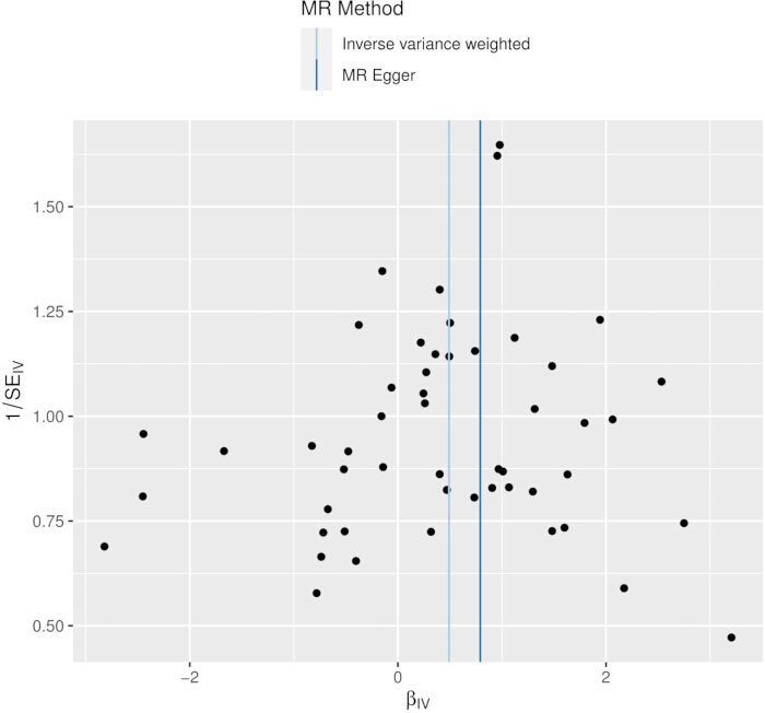
Figure 5. Funnel plot of SNP-specific MR estimates. This figure shows the distribution of SNP-specific MR estimates and allows visual assessment of symmetry across genetic instruments. MR, Mendelian randomization; IVW, inverse variance weighted. Please click here to view a larger version of this figure.
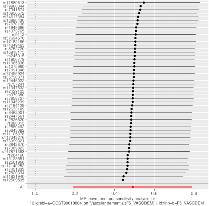
Figure 6. Leave-one-out sensitivity analysis. This figure shows the MR estimate after sequentially removing each SNP. The plot was used to assess whether the overall estimate was driven by any single genetic instrument. Please click here to view a larger version of this figure.
| No. | SNP | Gene | Chr. | EA | OA | EAF.IS | EAF.VD | IS β (SE) | VD β (SE) | F statistic | R² |
| 1 | rs10886430 | GRK5 | 10 | G | A | 0.118244 | 0.09536 | 0.1147 (0.0220) | -0.0172 (0.0852) | 27.18 | 5.61E-05 |
| 2 | rs10936572 | LOC107986051 | 3 | T | C | 0.179643 | 0.1235 | -0.0512 (0.0104) | 0.1444 (0.0743) | 24.24 | 5.01E-05 |
| 3 | rs11045239 | PDE3A | 12 | A | G | 0.492943 | 0.4629 | 0.0604 (0.0089) | 0.0303 (0.0494) | 46.06 | 9.51E-05 |
| 4 | rs11047532 | LOC105369698 | 12 | G | C | 0.305214 | 0.1513 | 0.0499 (0.0105) | 0.0159 (0.0689) | 22.59 | 4.66E-05 |
| 5 | rs11065836 | CUX2 | 12 | A | G | 0.159123 | 0.07442 | -0.0608 (0.0103) | 0.0245 (0.0929) | 34.84 | 7.20E-05 |
| 6 | rs11105378 | ATP2B1 | 12 | T | C | 0.203466 | 0.07522 | -0.0540 (0.0098) | -0.1174 (0.0916) | 30.36 | 6.27E-05 |
| 7 | rs117140252 | - | 14 | A | G | 0.041216 | 0.06988 | 0.1568 (0.0311) | 0.1498 (0.0967) | 25.42 | 5.25E-05 |
| 8 | rs117343276 | - | 10 | G | A | 0.030533 | 0.0431 | -0.0905 (0.0196) | -0.1449 (0.1233) | 21.32 | 4.40E-05 |
| 9 | rs11831940 | HDAC7 | 12 | A | G | 0.251914 | 0.3526 | 0.0631 (0.0130) | 0.1226 (0.0513) | 23.56 | 4.87E-05 |
| 10 | rs11880613 | DNM2 | 19 | A | G | 0.184857 | 0.1804 | -0.0613 (0.0110) | 0.1499 (0.0640) | 31.06 | 6.41E-05 |
| 11 | rs12445022 | LOC124903748 | 16 | A | G | 0.271667 | 0.3193 | 0.0605 (0.0112) | 0.0218 (0.0527) | 29.18 | 6.03E-05 |
| 12 | rs12509595 | - | 4 | C | T | 0.297929 | 0.3124 | 0.0577 (0.0091) | 0.1462 (0.0533) | 40.2 | 8.30E-05 |
| 13 | rs12633109 | - | 3 | T | G | 0.360897 | 0.3263 | 0.0436 (0.0089) | 0.0395 (0.0526) | 24 | 4.96E-05 |
| 14 | rs1275980 | KCNK3 | 2 | T | C | 0.498545 | 0.5481 | -0.0582 (0.0094) | -0.0128 (0.0495) | 38.33 | 7.92E-05 |
| 15 | rs13123551 | - | 4 | A | T | 0.616442 | 0.5065 | 0.0552 (0.0097) | 0.0818 (0.0493) | 32.38 | 6.69E-05 |
| 16 | rs147871383 | MIR99AHG | 21 | A | G | 0.02368 | 0.01925 | 0.2259 (0.0494) | 0.2534 (0.1903) | 20.91 | 4.32E-05 |
| 17 | rs16918175 | - | 10 | C | T | 0.104037 | 0.0811 | -0.0649 (0.0131) | 0.0332 (0.0895) | 24.54 | 5.07E-05 |
| 18 | rs17182166 | ACVR1 | 2 | T | G | 0.12494 | 0.137 | 0.0751 (0.0156) | -0.0046 (0.0703) | 23.18 | 4.79E-05 |
| 19 | rs1906779 | - | 15 | A | G | 0.211386 | 0.1239 | 0.0438 (0.0095) | -0.0342 (0.0758) | 21.26 | 4.39E-05 |
| 20 | rs1948696 | ITGB5 | 3 | C | T | 0.650138 | 0.6041 | -0.0459 (0.0091) | 0.0219 (0.0501) | 25.44 | 5.25E-05 |
| 21 | rs1973765 | LSP1 | 11 | C | T | 0.486717 | 0.4124 | 0.0441 (0.0092) | -0.0229 (0.0505) | 22.98 | 4.75E-05 |
| 22 | rs2429123 | CACNA1C, DCP1B | 12 | C | T | 0.729926 | 0.725 | 0.0473 (0.0098) | 0.0190 (0.0549) | 23.3 | 4.81E-05 |
| 23 | rs2447561 | - | 8 | T | A | 0.873442 | 0.8382 | -0.0589 (0.0116) | -0.0570 (0.0674) | 25.78 | 5.33E-05 |
| 24 | rs245015 | MSH3 | 5 | A | G | 0.685061 | 0.6562 | -0.0456 (0.0089) | 0.0065 (0.0519) | 26.25 | 5.42E-05 |
| 25 | rs2501968 | CENPQ | 6 | G | A | 0.465302 | 0.4229 | -0.0490 (0.0086) | -0.0879 (0.0498) | 32.46 | 6.71E-05 |
| 26 | rs2526620 | - | 7 | G | A | 0.252144 | 0.2459 | 0.0500 (0.0092) | 0.0505 (0.0576) | 29.54 | 6.10E-05 |
| 27 | rs284160 | TGFBR3 | 1 | A | G | 0.192644 | 0.1186 | 0.0572 (0.0096) | 0.1573 (0.0768) | 35.5 | 7.33E-05 |
| 28 | rs2842870 | PMF1, PMF1-BGLAP | 1 | C | T | 0.360398 | 0.3434 | -0.0446 (0.0087) | -0.0727 (0.0518) | 26.28 | 5.43E-05 |
| 29 | rs2880492 | NCOR2 | 12 | C | T | 0.035841 | 0.01984 | -0.1293 (0.0266) | -0.1917 (0.1781) | 23.63 | 4.88E-05 |
| 30 | rs35790371 | RBFOX1 | 16 | A | G | 0.005125 | 0.001903 | 0.5587 (0.1176) | 0.1447 (0.5420) | 22.57 | 4.66E-05 |
| 31 | rs5752720 | TTC28 | 22 | T | C | 0.28441 | 0.1844 | 0.0422 (0.0091) | -0.0311 (0.0635) | 21.51 | 4.44E-05 |
| 32 | rs57694670 | SH3PXD2A | 10 | G | A | 0.433638 | 0.3834 | -0.0507 (0.0086) | 0.0080 (0.0507) | 34.76 | 7.18E-05 |
| 33 | rs6462001 | - | 7 | T | G | 0.881494 | 0.8329 | -0.0765 (0.0151) | -0.0567 (0.0662) | 25.67 | 5.30E-05 |
| 34 | rs6843082 | - | 4 | A | G | 0.65294 | 0.6907 | -0.0438 (0.0092) | -0.0568 (0.0534) | 22.67 | 4.68E-05 |
| 35 | rs7091346 | SH3PXD2A | 10 | T | C | 0.45273 | 0.2664 | -0.0582 (0.0098) | -0.0143 (0.0552) | 35.27 | 7.28E-05 |
| 36 | rs7194129 | CFDP1 | 16 | T | C | 0.573691 | 0.5538 | 0.0399 (0.0084) | 0.0293 (0.0495) | 22.56 | 4.66E-05 |
| 37 | rs7341574 | ZFPM2 | 8 | T | C | 0.313243 | 0.3895 | 0.0463 (0.0094) | -0.0774 (0.0505) | 24.26 | 5.01E-05 |
| 38 | rs7451833 | - | 6 | G | A | 0.103042 | 0.1166 | 0.1280 (0.0220) | 0.1253 (0.0777) | 33.85 | 6.99E-05 |
| 39 | rs74617384 | LPA | 6 | T | A | 0.070999 | 0.04573 | 0.1415 (0.0281) | -0.0532 (0.1162) | 25.36 | 5.24E-05 |
| 40 | rs74849463 | PIK3C2B | 1 | T | C | 0.240949 | 0.2043 | 0.0445 (0.0092) | -0.0319 (0.0616) | 23.4 | 4.83E-05 |
| 41 | rs757241 | AFAP1-AS1 | 4 | C | G | 0.673377 | 0.6704 | -0.0681 (0.0145) | -0.0274 (0.0523) | 22.06 | 4.56E-05 |
| 42 | rs76099321 | CNNM2 | 10 | A | G | 0.052085 | 0.02979 | -0.0691 (0.0150) | -0.2215 (0.1464) | 21.22 | 4.38E-05 |
| 43 | rs7670136 | - | 4 | C | T | 0.571088 | 0.6269 | -0.0473 (0.0101) | 0.0391 (0.0509) | 21.93 | 4.53E-05 |
| 44 | rs77455924 | NTM | 11 | T | C | 0.056457 | 0.02996 | 0.1632 (0.0331) | 0.0444 (0.1477) | 24.31 | 5.02E-05 |
| 45 | rs7820334 | - | 8 | T | C | 0.246549 | 0.2949 | -0.0643 (0.0127) | -0.1327 (0.0648) | 25.63 | 5.29E-05 |
| 46 | rs7859727 | CDKN2B-AS1 | 9 | T | C | 0.518845 | 0.4151 | 0.0569 (0.0087) | 0.0281 (0.0498) | 42.77 | 8.83E-05 |
| 47 | rs7989823 | COL4A1, COL4A2 | 13 | C | A | 0.591615 | 0.6188 | 0.0527 (0.0089) | 0.0693 (0.0518) | 35.06 | 7.24E-05 |
| 48 | rs79960344 | - | 17 | G | T | 0.102808 | 0.1031 | 0.0651 (0.0130) | -0.1596 (0.0805) | 25.08 | 5.18E-05 |
| 49 | rs880315 | CASZ1 | 1 | C | T | 0.445525 | 0.4139 | 0.0416 (0.0089) | 0.0444 (0.0501) | 21.85 | 4.51E-05 |
| 50 | rs9112 | LOC100505841 | 5 | A | G | 0.436595 | 0.3573 | 0.0407 (0.0085) | -0.0274 (0.0523) | 22.93 | 4.74E-05 |
| 51 | rs979380 | - | 17 | A | G | 0.531844 | 0.6197 | -0.0417 (0.0084) | -0.0196 (0.0506) | 24.64 | 5.09E-05 |
| EAF.IS and EAF.VD denote the effect-allele frequencies in the ischemic stroke exposure and vascular dementia outcome datasets, respectively. F statistic = (β/SE)². Per-SNP R² = F/(F + N − 2), where N = 484,121. SNPs were selected using p < 5 × 10⁻⁶ and linkage disequilibrium clumping with r² < 0.001 within a 10,000 kb window. | |||||||||||
Table 1: Genetic instruments for ischemic stroke and corresponding SNP–outcome associations for VaD. The table lists the final 51 SNPs, including SNP ID, mapped gene, chromosome, alleles, EAF, SNP–trait estimates, F-statistics, and per-SNP R2. SNPs were selected at p < 5 × 10⁻⁶ and clumped at r2 < 0.001 within 10,000 kb. EAF.IS and EAF.VD denote effect-allele frequencies in the IS and VD datasets, respectively. Chr., chromosome; EA, effect allele; OA, other allele; EAF, effect-allele frequency; IS, ischemic stroke; VD, vascular dementia. Please click here to download this Table.
Supplementary Table 1. MR-PRESSO assessment of horizontal pleiotropy for the ischemic stroke–vascular dementia analysis. This table summarizes the MR-PRESSO analysis performed to assess global horizontal pleiotropy and potential outlier variants using the final harmonized dataset of 51 SNPs.Please click here to download this file.
Supplementary Table 2. Protocol steps and corresponding validating outputs. This table links each major step of the protocol to its corresponding representative output and reported location in the manuscript, demonstrating the implementation and validation of the analytical workflow.Please click here to download this file.
Discussion
This study presents a two-sample MR protocol for evaluating the potential causal association between IS and VaD using publicly available GWAS summary statistics. In the representative analysis, the IVW and weighted median methods supported a positive association between genetically predicted IS and VaD risk, whereas the MR-Egger estimate was directionally consistent but did not reach statistical significance. Therefore, these findings provide suggestive evidence of a possible causal effect, rather than definitive proof of causality.
The observed association is biologically plausible in the context of cerebrovascular injury. IS can lead to regional neuronal injury, impaired cerebral perfusion, and subsequent neurodegenerative changes. Previous studies have shown that VaDoften occurs in the setting of reduced cerebral blood flow or cerebrovascular damage13,14. Chronic cerebrovascular changes following IS may further contribute to cognitive decline and VaD risk15. In addition, post-stroke microvascular injury, inflammatory responses, and chronic neurovascular dysfunction may provide potential biological links between IS and VaD. However, the present MR protocol cannot directly establish these mechanisms, and the findings should be interpreted together with future mechanistic and clinical validation studies.
The MR-Egger estimate did not reach statistical significance. This finding should be interpreted cautiously rather than as directly contradicting the IVW and weighted median results. MR-Egger can provide estimates that are more robust to certain forms of directional pleiotropy, but it usually has lower statistical power, particularly when instrument effects are modest. In this analysis, the MR-Egger intercept did not indicate statistically significant directional horizontal pleiotropy, and the heterogeneity tests did not show substantial between-SNP heterogeneity. In addition, the MR-PRESSO global test showed no evidence of global horizontal pleiotropy. These sensitivity analyses reduce concern about measurable directional or global horizontal pleiotropy, but they do not exclude all possible sources of bias or establish causality.
The modest number of VaD cases should nevertheless be considered when interpreting these findings. Although the primary IVW analysis had an estimated post hoc power of 89.5% conditional on the observed effect size, this result is descriptive and should not be interpreted as a prespecified sample-size justification. The limited case count particularly reduced the precision of less efficient sensitivity estimators; the 80% minimum detectable effect for MR-Egger was an OR of 3.23, which was larger than its observed estimate. Accordingly, the non-significant MR-Egger result does not eliminate uncertainty regarding the magnitude of the association. These power calculations also do not address potential bias related to instrument validity, sample overlap, phenotype heterogeneity, or residual horizontal pleiotropy.
Several analytical steps are critical for the reliability of this MR workflow. First, the exposure and outcome GWAS datasets should be clearly identified using dataset IDs or accession information. Second, SNP selection and linkage disequilibrium clumping should be performed using predefined thresholds to obtain independent genetic instruments. Third, instrument strength should be assessed using F-statistics to reduce the risk of weak instrument bias. Fourth, allele harmonization is essential to ensure that SNP–exposure and SNP–outcome estimates correspond to the same effect allele. Finally, heterogeneity, horizontal pleiotropy, and leave-one-out analyses should be used to evaluate whether the primary estimate is influenced by inconsistent SNP effects, directional pleiotropy, or a single dominant genetic instrument.
Common sources of failure or bias in this workflow include insufficient exposure-associated SNPs, weak instruments, unavailable outcome SNPs, ambiguous allele alignment, palindromic variants, proxy SNP mismatch, heterogeneity across SNP-specific estimates, horizontal pleiotropy, population mismatch, phenotype heterogeneity, and possible sample overlap. These issues can be addressed by checking the GWAS dataset identifiers, applying consistent SNP selection and clumping thresholds, documenting proxy SNP use, inspecting harmonization outputs, summarizing F-statistics, and interpreting MR estimates together with heterogeneity, pleiotropy, and leave-one-out results. If substantial heterogeneity or pleiotropy is detected, the primary IVW estimate should be interpreted cautiously and additional sensitivity analyses or alternative datasets should be considered.
Potential sample overlap should also be considered. The exposure GWAS and FinnGen outcome GWAS were both derived from European-ancestry resources, and the extent of any participant overlap could not be quantified from the available summary statistics. Such overlap may bias two-sample MR estimates toward observational associations, particularly when instruments are not strongly associated with the exposure. This limitation should be considered when interpreting the representative result.
Compared with conventional observational cohort or case-control studies, MR can reduce confounding and reverse causality bias under valid instrumental variable assumptions. However, observational studies remain valuable for estimating disease incidence, temporal patterns, and clinical prognosis. Compared with randomized controlled trials or experimental models, MR can evaluate potential causal associations using existing genetic data when direct intervention studies are infeasible or unethical. Nevertheless, MR cannot directly reveal cellular mechanisms or replace mechanistic validation. Therefore, this protocol should be viewed as complementary to cohort studies, cross-sectional analyses, animal models, and cell experiments rather than as a substitute for them.
Previous studies have explored vascular risk factors and dementia-related outcomes using epidemiological and genetic approaches. For example, diabetes and hypertension have been associated with dementia risk in previous clinical and population-based research16. Existing MR-based studies have also investigated IS, VaD, and related comorbidity mechanisms. The present manuscript differs from these studies in its primary objective. Rather than aiming to identify new molecular targets or experimentally validate disease mechanisms, this article focuses on presenting a reproducible protocol for conducting a two-sample MR analysis using publicly available GWAS summary statistics.
This protocol has several limitations. First, the analysis was based on publicly available GWAS summary statistics, and the results may not be fully generalizable to non-European populations or datasets with different case definitions. Second, a relaxed SNP selection threshold (p < 5 × 10⁻⁶) was used to retain an adequate number of independent instruments for sensitivity analyses. Although all retained instruments had F-statistics >10, this threshold is less stringent than the conventional genome-wide significance threshold and may include variants with weaker or less robust exposure associations. Therefore, the representative findings should be interpreted as exploratory and suggestive rather than definitive evidence of causality. Third, although MR can reduce confounding and reverse causality bias, it cannot completely exclude horizontal pleiotropy, phenotype misclassification, sample overlap, or bias introduced by invalid instruments. Fourth, the non-significant MR-Egger estimate indicates that the causal interpretation should remain cautious. Fifth, this protocol does not include cell experiments, animal models, or independent cohort validation; these approaches would be valuable for clarifying biological mechanisms and clinical applicability.
In addition, IS was modeled as an overall phenotype. This representative protocol was not designed to identify whether any association is attributable to large-artery atherosclerotic stroke, small-vessel occlusion, cardioembolic stroke, or another subtype. Consequently, the result should not be interpreted as evidence of a subtype-specific effect. Future work should apply the same workflow to well-powered subtype-specific GWAS datasets using a prespecified, harmonized analysis plan.
Future applications of this protocol may extend beyond IS and VaD. The same workflow can be adapted to evaluate other cerebrovascular, neurodegenerative, metabolic, inflammatory, or cardiovascular exposure–outcome relationships when suitable GWAS summary statistics are available. Future studies may also extend this workflow by incorporating independent GWAS validation, bidirectional MR, multivariable MR, mediation MR, or integration with cohort-based and experimental evidence.
In summary, this protocol provides a reproducible workflow for conducting two-sample MR analysis using public GWAS summary statistics. The representative results provide suggestive evidence of a possible positive association between genetically predicted IS and VaD risk, mainly supported by the IVW and weighted median methods, while the MR-Egger estimate did not reach statistical significance. However, the findings should not be interpreted as definitive mechanistic proof. Independent population-based validation studies and experimental investigations are needed to further clarify the biological mechanisms and clinical relevance of this association.
Disclosures
The authors declare no competing financial interests. No artificial intelligence (AI) or large language model (LLM) tools were used in the writing, editing, or preparation of this manuscript.
Acknowledgements
The authors received no specific funding for this study.
Materials
| Name | Company | Catalog Number | Comments |
|---|---|---|---|
| FinnGen GWAS dataset | FinnGen | finn-b-F5_VASCDEM | Public GWAS dataset used as the outcome source for vascular dementia |
| IEU OpenGWAS database | MRC Integrative Epidemiology Unit, University of Bristol | ebi-a-GCST90018864 | Public GWAS dataset used as the exposure source for ischemic stroke |
| R software | R Foundation for Statistical Computing | Not Applicable | Statistical software used for MR analysis |
| RStudio | Posit Software, PBC | Not Applicable | Integrated development environment used to run R scripts |
| TwoSampleMR package | MRC Integrative Epidemiology Unit, University of Bristol | Not Applicable | R package used for instrument extraction, harmonization, MR analysis, and sensitivity analyses |
| MRPRESSO package | CRAN | Version 1.0 | R package used to assess global horizontal pleiotropy and potential outlier instruments |
| writexl package | CRAN | Not Applicable | R package used to export result tables as xlsx files |
References
- Sharma R, Lee K. Advances in treatments for acute ischemic stroke. BMJ. 2025;389:e076161.
- Zhu H, et al. Interleukins and ischemic stroke. Front Immunol. 2022;13:828447.
- Feske SK. Ischemic stroke. Am J Med. 2021;134(12):1457-1464.
- Lin HF, et al. Apolipoprotein E polymorphism in ischemic cerebrovascular diseases and vascular dementia patients in Taiwan. Neuroepidemiology. 2004;23(3):129-134.
- Semplicini A, et al. Hypertension and cerebrovascular diseases: a specific role of vascular protection for the prevention of dementia. J Cardiovasc Pharmacol. 2001;38(Suppl 2):S79-S82.
- Bulwa Z, et al. Management of blood pressure after acute ischemic stroke. Curr Neurol Neurosci Rep. 2019;19(6):29.
- Hosoki S, Tanaka T, Ihara M. Diagnostic and prognostic blood biomarkers in vascular dementia: from the viewpoint of ischemic stroke. Neurochem Int. 2021;146:105015.
- Yamagata K. Docosahexaenoic acid inhibits ischemic stroke to reduce vascular dementia and Alzheimer's disease. Prostaglandins Other Lipid Mediat. 2023;167:106733.
- Yeung S, Luo S, Iwagami M, Goto A. Introduction to Mendelian randomization. Ann Clin Epidemiol. 2025;7(1):27-37.
- Luo J, et al. Cardiovascular diseases and risk of dementia in the general population. Eur J Prev Cardiol. 2025:zwaf129. Available from: https://academic.oup.com/eurjpc
- Burgess S. Sample size and power calculations in Mendelian randomization with a single instrumental variable and a binary outcome. Int J Epidemiol. 2014;43(3):922-929. Available from: https://academic.oup.com/ije/article/43/3/922/757361
- Verbanck M, et al. Detection of widespread horizontal pleiotropy in causal relationships inferred from Mendelian randomization between complex traits and diseases. Nat Genet. 2018;50(5):693-698. Available from: https://www.nature.com/articles/s41588-018-0099-7
- Ng S, et al. Updates on vascular dementia. Stroke Vasc Neurol. 2025;10(5):542-550.
- Sanders AE, Schoo C, Kalish VB. Vascular Dementia. StatPearls Publishing; Treasure Island (FL); 2025. Available from: https://www.ncbi.nlm.nih.gov/books/
- Ho JP, Powers WJ. Contemporary management of acute ischemic stroke. Annu Rev Med. 2025;76(1):417-429.
- Yen FS, et al. Diabetes, hypertension, and the risk of dementia. J Alzheimers Dis. 2022;89(1):323-333.