Benzo[a]pyrene and Rheumatoid Arthritis: An Integrated Computational Investigation

Summary

This study employed an integrated computational toxicology approach to systematically investigate the link between Benzo[a]pyrene exposure and rheumatoid arthritis. The analysis identified five core target genes, revealed their enrichment in key immune pathways, and validated stable BaP-protein binding, elucidating potential molecular mechanisms for environmental pollutant-induced rheumatoid arthritis (RA).

Abstract

Polycyclic aromatic hydrocarbons (PAHs), ubiquitous environmental pollutants, are considered significant environmental factors contributing to the pathogenesis of RA. Benzo[a]pyrene (BaP), a key component of PAHs, may be associated with RA onset; however, the underlying toxicological mechanism remains to be fully elucidated. In this study, we systematically addressed this knowledge gap using an integrated approach combining network toxicology, machine learning, and molecular docking. Initially, a network toxicology analysis was conducted based on the molecular structure of BaP. By integrating and screening target information from multiple databases, 15 potential RA-related target genes of BaP were ultimately identified, and their interaction network was constructed. GO and KEGG enrichment analyses revealed that these genes were significantly enriched in biological processes such as leukocyte migration and immune cell signal transduction and were associated with the NF-κB and T cell receptor signaling pathways, among others. Subsequent topological analysis using the STRING database and Cytoscape software screened out five core genes (LCK, ZAP70, ITK, GZMA, and ITGAL), whose importance was further validated through machine learning. Molecular docking and molecular dynamics simulation results indicated that BaP exhibits strong binding affinity for the protein products of these target genes, resulting in the formation of conformationally stable complexes. In summary, this study employs an integrated computational approach to elucidate the potential mechanisms by which BaP may contribute to RA development, thereby offering a theoretical foundation for future investigations into the prevention and treatment of RA associated with environmental pollutants.

Introduction

RA is a common autoimmune disease characterized by chronic synovitis and pannus formation, which drive the progressive destruction of cartilage and bone erosion. These pathological changes lead to joint dysfunction, an increased risk of pathological fractures, and ultimately disability, thereby severely impairing the quality of life of affected individuals¹. While the etiology of RA is not fully understood, its pathogenesis is generally attributable to the combined effects of genetic (e.g., HLA-DR4 and HLA-DR1 gene subtypes) and environmental factors (e.g., smoking, alcohol consumption, Epstein-Barr virus infection, exposure to air pollution)². Epidemiological studies have established a significant association between PAHs from air pollution and an increased risk of RA onset³.

PAHs are common air pollutants originating from the incomplete combustion of substances such as coal, petroleum, natural gas, and tobacco, and are considered important environmental mediators of the pathogenesis of RA. They can bind to the aryl hydrocarbon receptor (AHR) complex in immune cells, leading to the exposure of nuclear localization signals, and the consequent translocation of the ligand–AHR complex into the nucleus. In the context of RA pathogenesis, PAH-bound AHR acts as a central environmental sensor that drives immune dysregulation through interconnected pathways. Upon activation, AHR forms heterodimers with ARNT and modulates CYP gene expression, initiating an inflammatory cascade⁴. This AHR activation simultaneously disrupts the balance between pro-inflammatory and regulatory T cells: on one hand, it triggers the AHR/Jag1/Notch signaling axis, enhancing Th17 cell cytokine release⁵. On the other hand, AHR directly binds to the GOT1 promoter to upregulate GOT1 expression, which induces hypermethylation of the FOXP3 locus and suppresses Treg differentiation⁶. The resulting Th17/Treg imbalance favors a pro-inflammatory environment. Moreover, AHR activation further amplifies Th2-type responses by increasing CCR8 expression and cytokines such as IL-4 and IL-13, which collectively perpetuate synovial inflammation and tissue damage⁷. Thus, AHR activation serves as a hub that links environmental PAH exposure to Th17/Treg/Th2 dysregulation, establishing a mechanistic bridge between genotype, environmental factors, and RA pathology.

In the atmosphere, PAHs exist as complex mixtures, with BaP serving as a key constituent. In human macrophages, BaP can induce CXCL8 (IL-8) production by promoting the binding of AHR to the CXCL8 promoter, subsequently inducing the expression of neutrophil chemotactic factors⁸. Additionally, BaP can upregulate Slug expression in fibroblast-like synoviocytes (FLS) from patients with RA in a dose-dependent manner, which exacerbates arthritis progression⁹. In wild-type mice, BaP promotes factor Receptor Activator of Nuclear-factor kappaB Ligand (RANKL)-mediated osteoclast (OC) activation by inducing CYP1A1 enzyme activity, ultimately leading to bone loss¹⁰. However, the precise mechanism underlying the role of BaP toxicity in RA pathogenesis remains unclear. We hypothesize that BaP promotes RA pathogenesis by directly interacting with key immune‑related target proteins and disrupting multiple signaling pathways involved in T cell activation, Th17/Treg balance, and inflammatory cytokine production, thereby linking environmental BaP exposure to synovial inflammation and joint destruction. Network toxicology is more suitable than traditional single-pathway experimental methods for this study because BaP likely acts on multiple immune-related targets and intersecting pathways. Compared to conventional experimental approaches that typically examine one pathway or a few targets at a time, network toxicology enables a holistic view of multi-target interactions and systemic effects, though its predictions are database-dependent and require experimental validation.

Existing research on the role of BaP in RA is mostly limited to single pathways or linear mechanistic descriptions, lacking integrated analysis of multi-target, multi-level network regulatory characteristics. Existing research on the role of BaP in RA is mostly limited to single pathways or linear mechanistic descriptions, lacking integrated analysis of multi-target, multi-level network regulatory characteristics. Therefore, holistic approaches such as network toxicology are needed to unravel the complex link between BaP exposure and RA pathogenesis^11,12,13. Nevertheless, there is a scarcity of network toxicology studies relating to environmental pollutant-induced diseases. The novelty of this study lies in integrating network toxicology, machine learning, and molecular docking to systematically investigate BaP‑mediated RA pathogenesis, rather than focusing on a single pathway or isolated targets. It identifies key hub genes through topological analysis combined with machine learning, and, for the first time, provides molecular‑level validation of the binding modes and thermodynamic stability between BaP and the products of each core gene.By systematically identifying the potential molecular mechanisms through which BaP may promote the occurrence and development of RA, this computational study aims to provide a theoretical basis for understanding environmental triggers of RA and for developing targeted therapeutic strategies. Compared with traditional single-pathway analyses, this integrated approach enables systematic evaluation of multi‑target interactions, offering broader applicability in studying complex environmental disease mechanisms. It should be noted, however, that our method prioritizes high‑confidence hub genes through intersection and topological analysis, which may inadvertently exclude biologically relevant candidate genes that do not simultaneously meet the selection thresholds. Future studies could explore complementary strategies, such as applying machine learning to the union set of predicted targets, integrating other omics data, or performing targeted experimental validation, to further confirm and expand upon our findings.

Protocol

Ethics statement
This study did not directly involve any human participants or animal subjects.

BaP Target acquisition
BaP was characterized by integrating data from multiple databases. The PubChem database (https://pubchem.ncbi.nlm.nih.gov/) was queried using the keyword "Benzo[a]pyrene" to obtain its chemical structure and canonical 2D structure (SMILES string: C1=CC=C2C3=C4C(=CC2=C1)C=CC5=C4C(=CC=C5)C=C3)¹⁴. Potential BaP targets were retrieved from the ChEMBL (https://www.ebi.ac.uk/chembl/), SEA (https://sea.bkslab.org/), and PharmMapper (http://lilab-ecust.cn/pharmmapper) databases^15,16,17. All predicted targets were restricted to the Homo sapiens proteome. Complete list of predicted BaP targets (n = 474) is provided in Supplementary Table S1. The complete analytical workflow is represented schematically in Figure 1.

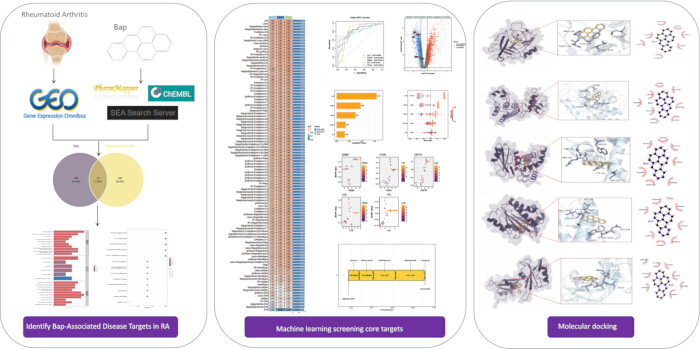
Figure 1. Flow-chart of dataset analysis in this paper, illustrating the overall workflow including data acquisition, preprocessing, differential expression analysis, network construction, and validation steps. Please click here to view a larger version of this figure.

Acquisition of RA-related targets
In this study, five RA datasets were acquired from the NCBI Gene Expression Omnibus (GEO) database(https://www.ncbi.nlm.nih.gov/gds/) using the keywords "Rheumatoid arthritis" and "Homo sapiens"¹⁸. Based on dataset size and experimental design, GSE77298 (RA: 16 samples; Control: 7 samples), GSE1919 (RA: 5 samples; Control: 5 samples), and GSE55235 (RA: 10 samples; Control: 10 samples) formed the training set for identifying differentially expressed genes (DEGs), while GSE12021 (RA: 24 samples; Control: 13 samples) and GSE55457 (RA: 13 samples; Control: 10 samples) served as the validation set. Further details on these datasets, such as platforms, samples, and GSE series, can be found in Table 1.

Data were standardized using the GEO2R online tool, generating log2-transformed expression matrices for subsequent analysis. To eliminate interference from different experimental batches, systematic biases between datasets were corrected using the ComBat function from the SVA package based on a parametric empirical Bayes framework. Principal Component Analysis (PCA) was subsequently used to verify the correction effect, showing significantly improved inter-batch sample clustering, and thus confirming the effective removal of batch effects. The merged and corrected data matrix was used for subsequent differential analysis.

GSE series	Samples	Platform	Group
GSE77298	16 RA and 7 controls	GPL570	Training cohort
GSE1919	5 RA and 5 controls	GPL91	Training cohort
GSE55235	10 RA and 10 controls	GPL96	Training cohort
GSE12021	24 RA and 13 controls	GPL96	Validation cohort
GSE55457	13 RA and 10 controls	GPL9	Validation cohort

Table 1: Summary of the five GEO datasets used in this study.
The table provides the GEO accession number (GSE series), sample composition (number of rheumatoid arthritis patients and healthy controls), platform identifier (GPL) for each dataset and assignment to either the training cohort or the validation cohort.

Weighted gene co-expression network analysis (WGCNA)
WGCNA was used to assess the co-expression network characteristics of the DEGs associated with RA¹⁹. Based on the batch-effect-corrected expression matrix, data preprocessing was first performed: low-variance genes with a standard deviation of less than 0.5 were removed, while sample and gene quality were evaluated using a function for assessing good samples and genes. Subsequently, hierarchical clustering was applied to identify and remove outlier samples. To construct a weighted co-expression network, a function for systematic evaluation of soft-thresholding power values was employed to systematically evaluate soft-thresholding power values ranging from 1 to 20. Power = 12 was selected as the optimal soft threshold (scale-free topology fit index R2 = 0.90), ensuring that the network topology adhered to a scale-free criterion. Based on this power value, an adjacency matrix was constructed, and the topological overlap matrix (TOM) was calculated. Genes were hierarchically clustered, and a dynamic tree‑cut algorithm was used to identify initial gene modules. Subsequently, similar modules were merged through the clustering of module eigengenes, resulting in a robust gene module network. All analyses were performed with a dedicated R package for weighted co-expression network analysis to ensure the reliability and reproducibility of network construction. An analysis of the intersection between DEGs/WGCNA hub genes and predicted BaP targets was undertaken to identify core targets of BaP associated with RA pathogenesis, which were visualized using Venn diagram software.

Identification of BaP-associated targets associated with RA pathogenesis
Intersection analysis was performed using an R package for Venn diagrams to identify targets of BaP that overlap with RA pathogenesis. These were imported into the STRING database to construct a protein–protein interaction (PPI) network, with the species set to "Homo sapiens" and the interaction confidence score set to > 0.7 to ensure high network reliability²⁰. This threshold was selected because it corresponds to a “high confidence” level in the STRING database, which balances the retention of biologically relevant interactions while minimizing false positives typically associated with lower confidence scores. A cutoff of > 0.7 has been widely adopted in network toxicology studies to prioritize robust and reproducible protein associations. The resulting TSV file was downloaded from the protein-protein interaction database (STRING) and imported into network visualization software (Cytoscape) for network visualization.Core proteins in the network were identified based on the ranking results generated by the Degree algorithm in the CytoHubba plugin and were used for subsequent analysis.

KEGG and GO enrichment analysis
The abbreviations of the genes associated with both BaP modulation and RA pathogenesis were converted to Entrez IDs using the "org.Hs.eg.db" annotation package in R. Subsequently, KEGG pathway enrichment analysis was performed using the clusterProfiler tool, with the significance threshold set to 0.05. Meanwhile, GO functional annotation covered the three major GO categories: Biological Process (BP), Cellular Component (CC), and Molecular Function (MF), and was performed using the enrichGO function, with both P-value and q-value cutoffs set to 0.05. It should be noted that no multiple testing correction was applied, as the primary objective of this exploratory analysis was to maximize the discovery of potentially relevant biological pathways and functional terms, thereby generating a broader set of testable hypotheses for future experimental validation. Finally, the enrichment analysis results were graphically displayed using the barplot and dotplot functions from the enrichplot package.

Machine learning-based validation of core genes
To assess the predictive capacity of the core genes associated with BaP and RA, and to maintain model transparency, we implemented a systematic machine learning workflow. Using the expression profiles of the selected core genes, predictive models were constructed with 11 distinct machine learning algorithms: Lasso regression (LR), Support Vector Machine (SVM), random forest (RF), glmBoost, stepwise Generalized Linear Model (GLM), ridge regression, elastic net (Enet), Gradient Boosting Machine (GBM), Linear Discriminant Analysis (LDA), eXtreme Gradient Boosting (XGBoost), and naive Bayes. Hyperparameters were optimized through five-fold cross-validation, with stratified sampling used to split the data into training and internal validation sets. A fixed random seed (set.seed(123)) was used throughout the machine learning workflow to ensure reproducibility of data splitting, cross‑validation folds, and model training. The key hyperparameters for each algorithm are provided in Supplementary Table S2. Model performance was evaluated using multiple metrics, including area under the curve (AUC), accuracy, and F1-score. To address the limitations inherent in single-model approaches, we applied a stacking ensemble strategy that integrated predictions from the best-performing base models. Recognizing the "black-box" nature of many machine learning models, we employed the SHapley Additive exPlanations (SHAP) algorithm to quantify each gene's contribution to the predictions. The magnitude and direction of SHAP values were used to interpret gene importance in the classification decisions, thereby enhancing the interpretability of the model outputs.

Molecular docking of BaP with core targets
To investigate the binding characteristics between BaP and the core gene products, molecular docking simulations were conducted. The three-dimensional structure of BaP (ligand) was obtained in SDF format from the PubChem database. Protein structures corresponding to the core targets were retrieved from the RCSB Protein Data Bank (https://www.rcsb.org/) in PDB format, selected according to their UniProt identifiers, with preference given to structures containing co-crystallized ligands or high-resolution coordinates. Prior to docking, protein preparation was carried out using PyMol, during which water molecules, co-crystallized ligands, and non-protein components such as ions were removed to prevent interference²¹. For proteins with co-crystallized ligands in their original PDB structures, the active site center was defined using the atomic coordinates of the bound ligand. For proteins without co-crystallized ligands, the active site center was determined based on coordinates of key residues reported in the literature to be critical for catalytic activity or inhibitor binding. The docking grid was centered at the defined active site coordinates, with a cubic box of 25 × 25 × 25 Å dimensions applied to each target. This standard 25 Å box size ensures full coverage of each active site with sufficient margin for ligand sampling while avoiding excessive computational cost. All docking calculations were executed with AutoDock Vina (version 1.2.5). The conformation exhibiting the most favorable Vina score was selected as the representative binding mode, and the corresponding binding energy was recorded. Three-dimensional binding poses were generated using PyMol (version 2.5.7), and two-dimensional interaction diagrams were produced using Discovery Studio (version 2021) to visualize key interactions, including hydrogen bonds and hydrophobic contacts.

Molecular dynamics simulation
Molecular dynamics simulations were carried out with Gromacs 2025.3, using the docking-derived complexes as starting structures. The protein atoms were modeled with the AMBER14SB force field, and water molecules were represented using the TIP3P model. Each protein–ligand complex was solvated in a cubic water box, with a minimum distance of 1 nm between the protein surface and the box boundary. Sodium or chloride ions were added as needed to achieve system electroneutrality. An initial energy minimization was conducted using a combination of steepest descent and conjugate gradient algorithms, each run for up to 10,000 steps. Long-range electrostatic interactions were computed via the Particle-Mesh Ewald (PME) method, while a cutoff distance of 1.0 nm was applied to both van der Waals and short-range electrostatic interactions. Following energy minimization, the systems were gradually equilibrated under NVT (constant volume and temperature) and NPT (constant pressure and temperature) conditions. Production runs of 100 ns were then performed under constant temperature and pressure, with a time step of 0.002 ps (2 fs) and a total of 50,000,000 steps. Each simulation was performed once (no replicates), as the primary aim was to assess the stability of the binding complexes under standard conditions. Temperature was maintained using the V-rescale thermostat, and pressure was controlled with the Parrinello–Rahman barostat. Throughout the simulation, a 1.0 nm cutoff was consistently applied for non-bonded interactions. To assess structural stability and flexibility, we calculated the root mean square deviation (RMSD) of atomic positions, the root mean square fluctuation (RMSF) per residue, the radius of gyration (Rg) as a measure of structural compactness, and the solvent-accessible surface area (SASA). All plots were generated using QtGrace.

Results

BaP Target acquisition
Data regarding the molecular structure of BaP were obtained from the PubChem database (Figure 2A). The potential biological targets of BaP were systematically predicted by integrating information from three complementary databases—ChEMBL, PharmMapper, and SEA—resulting in the identification of 474 potential targets (Figure 2B).

Discussion

RA is a complex autoimmune disease resulting from the interaction between genetic susceptibility and environmental factors. Among numerous environmental risk factors, PAHs, one of the most common air pollutants, are considered an important link connecting environmental exposure to RA onset. Earlier studies preliminarily revealed that PAHs can influence the balance of immune cell differentiation via the AHR pathway, as well as induce oxidative stress. BaP, a highly representative component of PAHs, has drawn significant a...

Materials

List of materials used in this article

Name	Company	Catalog Number	Comments
AutoDock Vina	https://vina.scripps.edu	1.2.5 (SCR_011958)	Molecular docking software
clusterProfiler (R package)	https://bioconductor.org/packages/clusterProfiler	4.10.0 (SCR_016884)	R package for enrichment analysis
CytoHubba (Cytoscape plugin)	https://apps.cytoscape.org/apps/cytohubba	0.1	Plugin for hub gene identification (Degree algorithm)
Cytoscape	https://cytoscape.org	3.10.1 (SCR_003032)	Network visualization software
Discovery Studio	Dassault Systèmes BIOVIA	2021	Software for 2D interaction diagram generation
enrichplot (R package)	https://bioconductor.org/packages/enrichplot	1.22.0 (SCR_021165)	R package for enrichment result visualization
GROMACS	https://www.gromacs.org	2025.3 (SCR_014565)	Molecular dynamics simulation software
limma (R package)	https://bioconductor.org/packages/limma	3.58.1 (SCR_010943)	R package for differential expression analysis
org.Hs.eg.db (R package)	https://bioconductor.org/packages/org.Hs.eg.db	3.18.0 (SCR_006442)	R annotation package for human gene identifiers
PyMol	Schrödinger, Inc	2.5.7 (SCR_000305)	Molecular visualization software
QtGrace	https://sourceforge.net/projects/grace/	0.2.6	Plotting tool for trajectory analysis
R (programming environment)	https://www.r-project.org	4.3.1 (SCR_001905)	Statistical computing software
STRING database	https://string-db.org	12 (SCR_005223)	Protein-protein interaction database
venn (R package)	https://cran.r-project.org/package=venn	1.11	R package for Venn diagram generation
WGCNA (R package)	https://cran.r-project.org/package=WGCNA	1.72 (SCR_003302)	Dedicated R package for weighted co-expression network analysis

References

- Zhao, Y., Chen, G. Y., Fang, M. Research trends of rheumatoid arthritis and depression from 2019 to 2023: a bibliometric analysis. J Multidiscip Healthc. 17, 4465-4474 (2024).
- Venetsanopoulou, A. I., Alamanos, Y., Voulgari, P. V., Drosos, A. A. Epidemiology of rheumatoid arthritis: genetic and environmental influences. Expert Rev Clin Immunol. 18 (9), 923-931 (2022).
- Beidelschies, M., et al. Polycyclic aromatic hydrocarbons and risk of rheumatoid arthritis: a cross-sectional analysis of the National Health and Nutrition Examination Survey, 2007 - 2016. BMJ Open. 13 (5), e071514(2023).
- Xi, X., et al. Polycyclic aromatic hydrocarbons affect rheumatoid arthritis pathogenesis via aryl hydrocarbon receptor. Front Immunol. 13, 797815(2022).
- Xia, M., et al. Vehicular exhaust particles promote allergic airway inflammation through an aryl hydrocarbon receptor-notch signaling cascade. J Allergy Clin Immunol. 136 (2), 441-453 (2015).
- Sun, L., et al. Particulate matter of 2.5 µm or less in diameter disturbs the balance of TH17/regulatory T cells by targeting glutamate oxaloacetate transaminase 1 and hypoxia-inducible factor 1α in an asthma model. J Allergy Clin Immunol. 145 (1), 402-414 (2020).
- Hew, K. M., et al. Childhood exposure to ambient polycyclic aromatic hydrocarbons is linked to epigenetic modifications and impaired systemic immunity in T cells. Clin Exp Allergy. 45 (1), 238-248 (2015).
- Podechard, N., et al. Interleukin-8 induction by the environmental contaminant benzo(a)pyrene is aryl hydrocarbon receptor-dependent and leads to lung inflammation. Toxicol Lett. 177 (2), 130-137 (2008).
- Lee, J., et al. A role for benzo[a]pyrene and Slug in invasive properties of fibroblast-like synoviocytes in rheumatoid arthritis: a potential molecular link between smoking and radiographic progression. Joint Bone Spine. 80 (6), 621-625 (2013).
- Iqbal, J., et al. Smoke carcinogens cause bone loss through the aryl hydrocarbon receptor and induction of Cyp1 enzymes. Proc Natl Acad Sci USA. 110 (27), 11115-11120 (2013).
- Chen, G. Y., et al. Mechanisms of total glucosides of paeony in alleviating methotrexate-induced liver injury. Drug Des Devel Ther. 19, 3407-3423 (2025).
- Chen, G. Y., et al. Prediction of Rhizoma Drynariae targets in the treatment of osteoarthritis based on network pharmacology and experimental verification. Evid Based Complement Alternat Med. 2021, 5233462(2021).
- Chen, G., Yan, Z., Wang, Y., Tao, Q. Rheumatoid Arthritis and Fibromyalgia Syndrome: A Bibliometric and Bioinformatics Perspective on Comorbidity Research. J Multidiscip Healthc. 18, 6811-6827 (2025).
- Kim, S., et al. PubChem 2023 update. Nucleic Acids Res. 51 (D1), D1373-D1380 (2023).
- Zdrazil, B., et al. The ChEMBL database in 2023: a drug discovery platform spanning multiple bioactivity data types and time periods. Nucleic Acids Res. 52 (D1), D1180-D1192 (2024).
- Keiser, M. J., et al. Relating protein pharmacology by ligand chemistry. Nat Biotechnol. 25 (2), 197-206 (2007).
- Liu, X., et al. PharmMapper server: a web server for potential drug target identification using pharmacophore mapping approach. Nucleic Acids Res. 38 (2), W609-W614 (2010).
- Barrett, T., et al. NCBI GEO: archive for functional genomics data sets—update. Nucleic Acids Res. 41 (D1), D991-D995 (2013).
- Langfelder, P., Horvath, S. Fast R functions for robust correlations and hierarchical clustering. J Stat Softw. 46 (11), 1-17 (2012).
- Szklarczyk, D., et al. The STRING database in 2023: protein-protein association networks and functional enrichment analyses for any sequenced genome of interest. Nucleic Acids Res. 51 (D1), D638-D646 (2023).
- wwPDB consortium. Protein Data Bank: the single global archive for 3D macromolecular structure data. Nucleic Acids Res. 47 (D1), D520-D528 (2019).
- Gentner, N. J., Weber, L. P. Intranasal benzo[a]pyrene alters circadian blood pressure patterns and causes lung inflammation in rats. Arch Toxicol. 85 (4), 337-346 (2011).
- Ordóñez, D., et al. Cell-mediated cytotoxicity in Lyme arthritis. Arthritis Rheumatol. 75 (5), 782-793 (2023).
- Zheng, Y., et al. Role of the granzyme family in rheumatoid arthritis: current insights and future perspectives. Front Immunol. 14, 1137918(2023).
- Wang, H., et al. Triple knockdown of CD11a, CD49d, and PSGL1 in T cells reduces CAR-T cell toxicity but preserves activity against solid tumors in mice. Sci Transl Med. 17 (782), eadl6432(2025).
- So, T., et al. Antigen-independent signalosome of CARMA1, PKCθ, and TNF receptor-associated factor 2 (TRAF2) determines NF-κB signaling in T cells. Proc Natl Acad Sci USA. 108 (7), 2903-2908 (2011).
- Genheden, S., Ryde, U. The MM/PBSA and MM/GBSA methods to estimate ligand-binding affinities. Expert Opi Drug Discov. 10 (5), 449-461 (2015).
Access restricted. Please log in or start a trial to view this content.