Transcriptomic Profiling and Bioinformatic Analysis of Bone Marrow Samples to Identify Chemotherapy Resistance Signatures in Acute Myeloid Leukemia

Summary

This protocol presents a standardized bioinformatic workflow to analyze transcriptomic alterations in acute myeloid leukemia (AML). The goal is to compare newly diagnosed and relapsed bone marrow samples and prioritize molecular signatures associated with chemotherapy resistance and disease progression for subsequent investigation.

Abstract

Acute myeloid leukemia (AML) is a highly heterogeneous hematologic malignancy in which relapse and acquired chemoresistance remain major causes of treatment failure. This article presents a bioinformatic protocol for transcriptomic analysis of bone marrow aspirates. The primary goal of the protocol is to provide a standardized workflow to identify molecular signatures associated with disease progression and therapy resistance in relapsed AML. The pipeline details the computational procedures for comparing unpaired bone marrow samples, demonstrated using sequencing data from five newly diagnosed cases and four relapsed cases. This method outlines the essential steps for processing RNA sequencing data, performing differential gene expression analysis, and conducting downstream functional evaluations. Applying this workflow identified 2,025 differentially expressed genes (DEGs), including FOXC1, HOXA11, HOXA11-AS, and AXL, as candidate transcripts associated with relapse in this representative dataset. Functional and network analyses further prioritized gene sets and interaction hubs related to small GTPase signaling, inflammatory signaling, extracellular matrix interactions, and RNA biosynthetic processes. Overall, this methodology provides a reproducible computational pipeline for mapping transcriptomic signatures associated with relapsed AML and for generating hypotheses that require subsequent experimental validation.

Introduction

Acute myeloid leukemia (AML) is a group of clonal malignant neoplasms originating from hematopoietic stem/progenitor cells, characterized by abnormal proliferation of immature myeloid cells in the bone marrow and suppression of hematopoietic differentiation^1,2,3. Although current standard induction chemotherapy (such as cytarabine combined with anthracyclines) can induce complete remission in most patients, the relapse rate remains as high as 50%–70%, and the prognosis for relapsed patients is significantly compromised^4,5,6. Acquired chemotherapy resistance is associated with AML treatment failure, necessitating an in-depth analysis of the molecular signatures linked to this process to improve therapeutic strategies and patient survival rates^7,8.

In the wider body of literature, existing studies indicate that chemotherapy resistance in AML is not limited to the upregulation of drug efflux pumps or abnormal drug metabolism but is also linked to the survival maintenance of leukemia stem cells (LSCs), the formation of epithelial-mesenchymal transition (EMT)-like phenotypes within the hematological niche, and interactions with the bone marrow microenvironment^9,10,11. For instance, LSC populations exhibit high self-renewal capacity and quiescence, which is associated with inherent resistance to cell cycle-specific chemotherapeutic agents¹². Additionally, the upregulation of receptor tyrosine kinases, such as AXL, has been associated with resistance in FLT3-ITD+ AML, occurring alongside the activation of PI3K/AKT and MAPK pathways and enhanced anti-apoptotic capabilities^13,14. Metabolic reprogramming and epigenetic remodeling have also been recognized as important regulatory axes in resistance formation. Evidence suggests that AML cells during relapse may adapt to chemotherapy-induced oxidative stress and DNA damage through enhanced oxidative phosphorylation (OXPHOS) activity, modulated NAD⁺/NADH ratios, and altered histone modification states^15,16,17. Inflammatory factors in the bone marrow microenvironment, such as IL-6 and CXCL8, are also associated with LSC survival and chemotherapy resistance, often occurring in coordination with the activation of STAT3/NF-κB signaling pathways^11,18.

Despite these recognized mechanisms, the transcriptomic changes associated with AML relapse and chemoresistance remain incompletely characterized, particularly when metabolic, epigenetic, and bone marrow microenvironment-related signals are evaluated together in clinical samples. This workflow addresses this need by prioritizing candidate DEGs, pathways, and regulatory networks associated with the transition from initial diagnosis to clinical relapse. The approach integrates differential expression analysis, gene set enrichment analysis (GSEA), and protein-protein interaction (PPI) network construction to map system-wide transcriptional reprogramming and to nominate candidates for subsequent mechanistic validation.

The overall goal of this method is to present a standardized, reproducible bioinformatics pipeline for comparing the bulk transcriptomes of newly diagnosed versus relapsed AML bone marrow samples. The rationale behind using this in silico technique is its capacity to capture unbiased, genome-wide transcriptional events, moving beyond the limitations of single-pathway analyses to prioritize complex, multidimensional regulatory networks. This technique offers significant advantages over alternative methods, such as microarrays or targeted multiplex qPCR panels, by providing a higher dynamic range, the ability to detect novel transcripts, and precise quantification of gene expression without the limitations of pre-designed probes^19,20. To determine whether this method is appropriate for their application, readers should note that this pipeline is specifically designed for investigators processing bulk RNA sequencing data from paired or unpaired clinical cohorts, such as tissue aspirates. It is suitable for identifying broad resistance-associated signatures and candidate regulatory networks, whereas researchers requiring cell-type-specific or spatial resolution would need to use complementary single-cell or spatial sequencing workflows. Ultimately, this computational protocol enables the prioritization of candidate genes, pathways, and regulatory networks for subsequent experimental investigation.

Protocol

All methods involving the use of human tissue sampling were performed in compliance with institutional guidelines and the Declaration of Helsinki (revised in 2013). The clinical bone marrow samples were obtained with approval from the institutional ethics committee (Approval Nos. TY-ZKY2024-116-01 and TY-ZKY2024-116-02).

1. Clinical Sample Collection and Patient Classification

1. Select bone marrow aspirate specimens from patients formally diagnosed with acute myeloid leukemia (AML) based on World Health Organization (WHO) classification criteria.
2. Apply specific inclusion and exclusion criteria during patient selection to ensure cohort homogeneity and reproducibility. Include adult patients with primary AML, and exclude patients with secondary AML, acute promyelocytic leukemia, or a prior history of other malignancies (Table 1).
3. Assign the collected sample to the newly diagnosed group if the patient presents with previously untreated AML at the time of initial clinical diagnosis.
4. Assign the collected sample to the relapsed group if the patient demonstrates a reappearance of leukemic blasts in the peripheral blood or greater than 5% blasts in the bone marrow following a documented complete remission.
5. Collect the de-identified residual bone marrow samples immediately following the routine clinical bone marrow aspiration procedure.
   NOTE: In the demonstration of this specific protocol, nine consecutive specimens (five newly diagnosed and four relapsed) were collected from September 2024 to September 2025. Because this utilized only de-identified residual clinical samples, the ethics committee waived the requirement for written informed consent.
6. Process the collected bone marrow aspirate immediately for RNA preservation using a standard phenol-guanidinium lysis method²¹.
   1. Transfer the freshly collected bone marrow aspirate into a collection tube containing an anticoagulant. Shake the tube to thoroughly mix the aspirate and the anticoagulant.
   2. Extract a measured volume of the anticoagulated sample and add it to a commercial phenol-guanidinium lysis reagent. Maintain a volume ratio of 3 parts lysis reagent to 1 part sample.
      CAUTION: The phenol-guanidinium lysis reagent contains toxic and corrosive chemicals that can cause severe burns and tissue damage. Perform all reagent handling inside a chemical fume hood while wearing appropriate personal protective equipment.
   3. Shake the tube vigorously to completely homogenize the sample and the lysis reagent. Ensure the mixture is fully blended and verify that no visible clots remain in the solution.
   4. Snap-freeze the homogenized sample immediately by submerging the tube in liquid nitrogen.
      CAUTION: Liquid nitrogen is extremely cold and can cause severe frostbite upon contact. Wear cryogenic gloves and a full face shield when handling liquid nitrogen.
7. Transfer the snap-frozen samples to a -80 °C freezer for long-term storage prior to the downstream RNA isolation and transcriptome sequencing pipeline. This represents a safe point at which the experiment can be paused and restarted later.
   NOTE: The workflow presented in this protocol focuses entirely on generating computational resistance signatures. No independent experimental validation, such as real-time quantitative PCR (RT-qPCR), was performed on the key differentially expressed genes identified through this specific pipeline.

2. RNA Quality Control and Library Preparation

1. Assess the RNA integrity using a microfluidic capillary electrophoresis system. For this representative workflow, include RNA samples with an RNA integrity number (RIN) ≥ 6.0, A260/280 ratio between 1.8 and 2.1, and no visible degradation peak. Record the measured RIN and purity ratios for each sample before library preparation.
2. Input 1 µg of total RNA per sample for the library preparation. Purify the mRNA from the total RNA utilizing poly-T oligo-attached magnetic beads to enrich for polyA-tailed transcripts.
3. Fragment the enriched mRNA using divalent cations. Incubate the mixture at 94 °C for 15 min in a 5X first-strand synthesis reaction buffer.
4. Synthesize the first-strand cDNA using random hexamer primers and a reverse transcriptase lacking RNase H activity.
5. Degrade the RNA template strand using RNase H. Synthesize the second-strand cDNA utilizing DNA Polymerase I and dNTPs in a 20 µL reaction system.
6. Incubate the second-strand synthesis reaction at 16 °C for 1 h. Centrifuge the reaction mixture briefly at 2,000 x g to collect the liquid at the bottom of the tube.
7. Convert the remaining overhangs into blunt ends utilizing exonuclease and polymerase activities. Adenylate the 3' ends of the DNA fragments and ligate adaptors with hairpin loop structures to prepare for hybridization.
8. Purify the library fragments using magnetic solid-phase reversible immobilization beads to preferentially select cDNA fragments 370–420 bp in length.
9. Perform ethanol washes during the bead purification. Centrifuge the tubes at 2,000 x g for 30 s to collect and completely remove any residual ethanol prior to the final elution.
10. Perform PCR amplification using a high-fidelity DNA polymerase, universal PCR primers, and sample-specific index primers.
11. Execute the PCR thermal profile with an initial denaturation at 98 °C for 30 s. Follow this with 12 cycles of 98 °C for 10 s, 60 °C for 30 s, and 72 °C for 30 s, ending with a final extension at 72 °C for 5 min.
12. Purify the PCR products again using the magnetic beads. Apply the identical centrifugation parameters from step 2.9 to obtain the final library.
13. Quantify the initial library concentration using a fluorometer. Dilute the final library to a concentration of 1.5 ng/µL.
14. Mix the diluted library thoroughly. Centrifuge the mixture at 10,000 x g for 1 min at 4 °C to remove any remaining debris before the final analysis.
15. Assess the insert size of the library using the microfluidic capillary electrophoresis system.
16. Quantify the effective concentration of the library accurately via real-time quantitative PCR (qRT-PCR) upon confirming the insert size meets expectations. Ensure the concentration is higher than 1.5 nM to guarantee library stability and sequencing quality.
    NOTE: This represents a safe point at which the experiment can be paused. The prepared libraries can be stored at -20 °C until clustering and sequencing.

3. Clustering and Transcriptome Sequencing

1. Perform the clustering of the index-coded samples on an automated cluster generation system. Use a commercial paired-end cluster kit according to the manufacturer’s instructions.
2. Sequence the library preparations on a high-throughput sequencing platform following successful cluster generation. Generate 150 base pair (bp) paired-end reads.

4. Data Quality Control and Reads Mapping

1. Assess the quality of the raw data (FASTQ format) using fastp v0.23.2 for raw-read quality control and filtering. Record the command-line parameters in an analysis log. In this workflow, clean reads were generated by removing adapter-containing reads, reads containing poly-N sequences, and low-quality reads using identical filtering settings across samples. A representative paired-end command is provided in Supplementary File 1.
2. Process the raw reads through an automated pre-processing software. Obtain clean reads by removing reads containing adapters, reads containing poly-N sequences, and low-quality reads. Use identical filtering parameters for all samples and record the retained read number, Q20, Q30, and GC content after filtering.
3. Calculate the Q20, Q30, and GC content of the clean data. Define potential batch variables before downstream analysis, including sample collection date, RNA extraction date, library preparation batch, sequencing lane, and sequencing run.
4. Evaluate batch effects by PCA and sample-to-sample correlation analysis using normalized expression values. If samples cluster primarily by technical variables rather than clinical state, document the affected variable and include it as a covariate in the differential expression design formula or apply an established batch-adjustment method before downstream visualization.
5. Acquire the reference genome (Homo sapiens, GRCh38) and the corresponding Ensembl release 109 gene annotation files for read alignment.
6. Build the index of the reference genome using HISAT2 v2.0.5.
7. Align the paired-end clean reads to the reference genome using HISAT2 v2.0.5. Use this splice-aware alignment approach to generate a database of splice junctions based on the gene model annotation file.

5. Novel Transcript Prediction and Gene Expression Quantification

1. Assemble the mapped reads of each sample using StringTie v1.3.3b in a reference-based approach. Utilize this tool to assemble and quantitate full-length transcripts representing multiple splice variants for each gene locus.
2. Count the number of reads mapped to each gene using featureCounts v1.5.0-p3. Use the resulting raw integer read-count matrix as the input for downstream differential expression analysis.
3. Configure featureCounts v1.5.0-p3 for paired-end sequencing data using the paired-end option (e.g., -p). Provide the downloaded GRCh38 GTF annotation file to define the correct genomic feature boundaries.
4. Calculate the Fragments Per Kilobase of transcript per Million mapped reads (FPKM) for each gene. Use FPKM values only for descriptive visualization, PCA, heatmap display, and exploratory expression summaries; do not use FPKM values as the input matrix for DESeq2 differential expression testing.

6. Differential Gene Expression Analysis

1. Perform differential expression analysis between the newly diagnosed and relapsed groups using R v3.5.0 and the DESeq2 R package v1.20.0. Import the raw read count matrix generated in step 5.2 into the R environment, and retain FPKM values only for visualization and exploratory analyses.
2. Construct the specialized dataset object required by the analysis package. Execute the specific command (e.g., DESeqDataSetFromMatrix()) to bind the count data matrix with the corresponding sample metadata table.
3. Define the experimental design formula within the software object. Specify the clinical state (newly diagnosed versus relapsed) as the primary variable for comparison (e.g., design = ~ condition). If a technical batch variable is identified in step 4.3 and is not completely confounded with clinical state, include it in the design formula (e.g., design = ~ batch + condition).
4. Execute the core differential expression analysis function (e.g., DESeq()). Allow the software to automatically perform size factor estimation, dispersion estimation, and negative binomial Wald test fitting²².
5. Extract the results table utilizing the result extraction function (e.g., results()). Specify the contrast argument to define the exact comparison (relapsed versus newly diagnosed).
6. Adjust the resulting P-values to control for the false discovery rate. Utilize the integrated Benjamini and Hochberg procedure automatically applied by the software package²³.
7. Filter the extracted results table to isolate the significant differentially expressed genes (DEGs). Assign any gene with an adjusted P-value < 0.05 and an absolute log₂ fold change > 1 as significantly differentially expressed.

7. Gene Ontology (GO) Enrichment Analysis

1. Perform Gene Ontology (GO) enrichment analysis of the identified DEGs using clusterProfiler v3.8.1 and org.Hs.eg.db v3.6.0. Input the list of Entrez gene IDs corresponding to the significant DEGs identified in step 6.7.
2. Execute the GO enrichment function (e.g., enrichGO()). Specify the required parameters, including the appropriate background organism database (e.g., OrgDb = org.Hs.eg.db), the specific ontology domain (Biological Process, Cellular Component, or Molecular Function), and the adjusted P-value cutoff (0.05).
3. Ensure the algorithm applies the necessary corrections during the enrichment calculation. Confirm that the software internally corrects for gene length bias and adjusts the P-values using the Benjamini and Hochberg method²⁴.
4. Consider GO terms with a corrected P-value less than 0.05 as significantly enriched. Generate a dot plot or bar chart utilizing the package's integrated visualization functions to display the top enriched GO terms.

8. Kyoto Encyclopedia of Genes and Genomes (KEGG) Pathway Enrichment Analysis

1. Utilize a comprehensive database resource dedicated to understanding high-level biological system functions to identify the dysregulated pathways. Prepare the identical list of significant DEG Entrez IDs utilized in step 7.1.
2. Execute the KEGG enrichment function (e.g., enrichKEGG()) within the functional annotation R package.
3. Define the critical parameters within the function call. Set the organism code strictly to human (e.g., organism = 'hsa') and define the P-value adjustment method (e.g., pAdjustMethod = 'BH').
4. Extract the statistically significant KEGG pathways. Filter the output to retain only those pathways demonstrating a corrected P-value less than 0.05.
5. Visualize the most heavily enriched KEGG pathways. Utilize the integrated plotting functions (e.g., dotplot()) to map the statistical significance and gene counts associated with each pathway.

9. Gene Set Enrichment Analysis (GSEA)

1. Prepare the pre-ranked gene list required for the analysis. Calculate the ranking metric for all expressed genes using the signed -log10(P-value) multiplied by the sign of the log₂ fold change derived from the differential expression analysis.
2. Launch a local installation of the Broad Institute GSEA software v4.2.3. Input the newly generated pre-ranked gene list into the software interface²⁵.
3. Download the required predefined gene sets. Acquire the Gene Ontology (GO) and Kyoto Encyclopedia of Genes and Genomes (KEGG) datasets from the Molecular Signatures Database (MSigDB, version 7.5.1)²⁶.
4. Configure the software parameters to perform the statistical enrichment test. Set the number of permutations to 1,000 and select the permutation type as 'gene_set'.
5. Execute the analysis algorithm to determine if the predefined gene sets show a statistically significant, concordant difference between the newly diagnosed and relapsed biological states.
6. Evaluate the statistical significance of the generated enrichment profiles. Define significant gene sets using strict thresholds: a normalized enrichment score (NES) absolute value > 1.0, a nominal P-value < 0.05, and a false discovery rate (FDR) q-value < 0.25.

10. Protein-Protein Interaction (PPI) Network Analysis

1. Access the STRING database for known and predicted protein-protein interactions. In this workflow, the PPI analysis was performed with STRING v11.5²⁷.
2. Input the list of Entrez gene IDs or official gene symbols for the significant differentially expressed genes (identified in step 6.7) into the database search interface. Select Homo sapiens as the target organism.
3. Configure the network construction parameters to ensure high-quality interactions are retrieved. Set the minimum required interaction score to a high confidence threshold (score > 0.700).
4. Export the resulting interaction network data to a local directory. Save the interaction map as a standard tabular file (e.g., TSV format).
5. Import the exported interaction data into Cytoscape v3.9.1 for network visualization and analysis²⁸.
6. Filter the constructed network to improve visualization clarity and highlight key regulatory hubs. Remove any disconnected nodes or orphan genes that do not exhibit continuous interactions meeting the established confidence threshold.

Results

Clinical Cohort and Sequencing Validation

The successful execution of the upstream RNA extraction and library preparation protocol (Figure 1) was confirmed by sequencing yield and quality metrics. In this representative dataset, bone marrow samples from five newly diagnosed AML patients and four relapsed AML patients yielded an average of approximately 6.0 GB of raw data per sample. Quality control assessment (Table 2) confirmed that base quality and read depth met the thresholds required for downstream bioinformatic analysis9. Low RNA integrity (for example, RIN < 6.0), low mapping rates, or high transcript degradation bias would represent suboptimal input quality and would compromise the reliability of downstream differential expression analysis.

Global Transcriptomic Variance and PCA

To assess global transcriptome variance and inspect clinical grouping, PCA was performed on the normalized expression data. In this representative dataset, the newly diagnosed and relapsed groups showed separation in two-dimensional space (Figure 2A)²⁰, with PC1 and PC2 accounting for 23.82% and 18.75% of the total variance, respectively. The Venn diagrams in Figure 2B,C provide an additional descriptive summary of genes detected across samples within the newly diagnosed and relapsed groups, supporting sample-level reproducibility checks before downstream differential expression analysis. Because the cohort was small and unpaired, PCA separation was interpreted as an illustrative workflow output rather than definitive evidence of disease-state-specific biology.

Differential Expression Gene (DEG) Analysis

Applying the established protocol thresholds (|log₂FC| ≥ 1 and adjusted P-value ≤ 0.05) to the DESeq2 output identified 2,025 DEGs, comprising 772 upregulated and 1,253 downregulated genes in the relapsed group (Figure 3A). Candidate transcripts with high variation included FOXC1 (log₂FC = 7.55, P = 4.92 x 10^-5), HOXA11 (log₂FC = 7.76), HOXA11-AS (log₂FC = 7.23), and AXL (log₂FC = 3.50), alongside downregulated RHOB, PTX3, and CXCL8. Existing literature links several of these genes to AML stemness, signaling, or therapy response^13,29; however, the present workflow identifies them only as relapse-associated candidate transcripts. Any definitive mechanistic role in clinical resistance requires subsequent independent functional validation.

Functional and Pathway Enrichment (GO, KEGG, and GSEA)

The functional annotation protocol mapped the DEGs to broader biological systems. GO analysis identified enrichment of terms related to small GTPase-mediated signal transduction, metal ion transport, and chromatin assembly (Figure 4A–C). KEGG pathway mapping identified associations with ECM-receptor interactions and cytokine-cytokine receptor interactions (Figure 4D). GSEA showed enrichment of RNA biosynthetic processes in the relapsed group and enrichment of energy metabolism pathways in the newly diagnosed group (Figure 5A). These enrichment results provide a descriptive roadmap of altered gene sets and should be interpreted as hypothesis-generating associations rather than proven drivers of relapse.

Protein-Protein Interaction (PPI) Network Construction

The initial STRING network contained 56 nodes and 193 interactions. After removal of disconnected or orphan nodes, the displayed Cytoscape subnetwork contained 42 nodes and 136 interactions (Figure 5B). Network modular analysis prioritized TP53, CCL2, CXCL8, and IL6 as central mathematical hubs with the highest number of interactions. Because the PPI network relies on database-predicted interaction scores (e.g., ATF3 score: 0.982), hub identification should be interpreted as target prioritization for future empirical studies rather than direct evidence of p53-mediated apoptosis evasion or other resistance mechanisms.

The raw RNA sequencing data generated in this protocol have been deposited in the Figshare repository and are publicly accessible via the following DOI: https://doi.org/10.6084/m9.figshare.30655814. The processed data and associated analysis files are included in the article and its supplementary materials. Representative command-line parameters and analysis settings used to reproduce the computational workflow are provided as Supplementary File 1. All data supporting the findings of this study are available without restriction.

Patient ID	Age (Years)	Sex	Molecular Mutations	Survival/Follow-up (Months)	Clinical Status
R_AML_1	70	Male	FLT3-ITD (+)	22	Deceased
R_AML_2	29	Female	NPM1 (+)	11	Alive
R_AML_3	40	Male	CEBPA (+)	17	Alive
R_AML_4	55	Female	Triple Negative*	24	Deceased

Table 1: Demographic and Clinical Characteristics of Patients in the Relapsed AML (R_AML) Group. Table 1 summarizes the demographic and clinical features of the relapsed AML cohort used in the representative analysis, including patient-level clinical characteristics relevant to interpretation of the transcriptomic workflow.

Sample	Library	Raw_reads	Raw_bases	Clean_reads	Clean_bases	Error_rate	Q20	Q30	GC_pct
AML_1	FRAS25 0244891-1r	48705066	7.31G	47807532	7.17G	0.01	99.35	97.48	47.48
AML_2	FRAS25 0244896-1r	42969940	6.45G	42237962	6.34G	0.01	99.35	97.44	46.74
AML_3	FRAS2502 44906-1r	48738386	7.31G	47744462	7.16G	0.01	99.36	97.48	47.28
AML_4	FRAS250 244915-1r	48723650	7.31G	47688240	7.15G	0.01	99.29	97.26	47.45
AML_5	FRAS2502 44920-1r	49508198	7.43G	47740308	7.16G	0.01	99.37	97.53	47.73
R_AML_1	FRAS2502 44892-1r	47879408	7.18G	46671584	7.0G	0.01	99.39	97.49	47.63
R_AML_2	FRAS2502 70005-1r	47657378	7.15G	46957882	7.04G	0.01	99.39	97.49	50.5
R_AML_3	FRAS250 405722-1r	58754766	8.81G	56867112	8.53G	0.01	99.38	97.42	46.52
R_AML_4	FRAS2502 44902-1r	48491122	7.27G	47469334	7.12G	0.01	99.23	97.21	46.43

Table 2: Summary of data quality. Table 2 reports sequencing quality metrics for each sample, including read yield, base quality, GC content, and mapping-related quality-control information used to determine whether samples were suitable for downstream analysis.

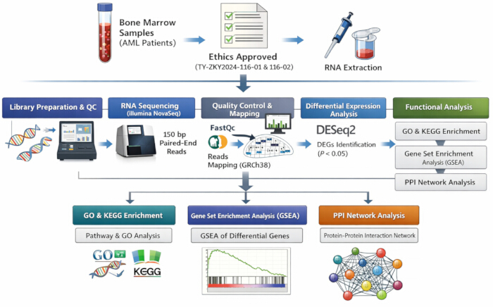
Figure 1: Workflow of the protocol. The workflow summarizes the major experimental and computational stages, including clinical sample collection, RNA quality control, library preparation and sequencing, read processing and alignment, transcript quantification, differential expression analysis, GO/KEGG enrichment, GSEA, and PPI network construction. Please click here to view a larger version of this figure.

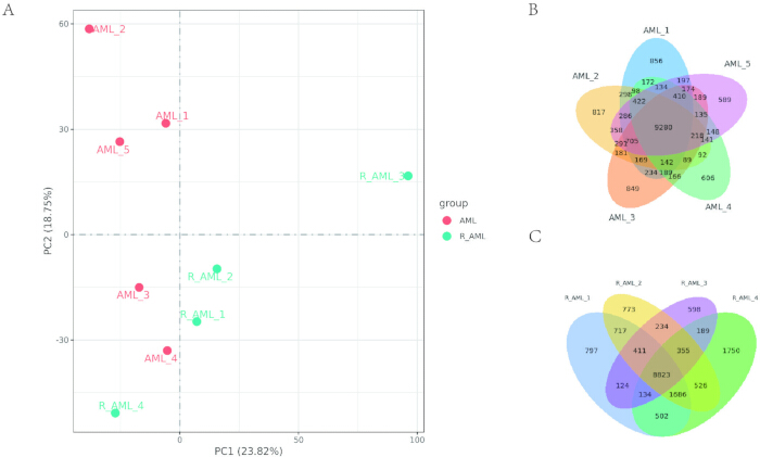
Figure 2: Quantitative analysis of samples. (A) Principal component analysis (PCA) was performed to evaluate intergroup differences and within-group sample reproducibility. PCA was conducted using linear algebraic methods based on normalized gene expression values across all samples. (B, C) Venn diagrams showing genes detected across samples in the AML and R_AML groups, respectively. Sample-restricted regions indicate genes detected in individual samples, while overlapping areas represent genes commonly detected across two or more samples. Please click here to view a larger version of this figure.

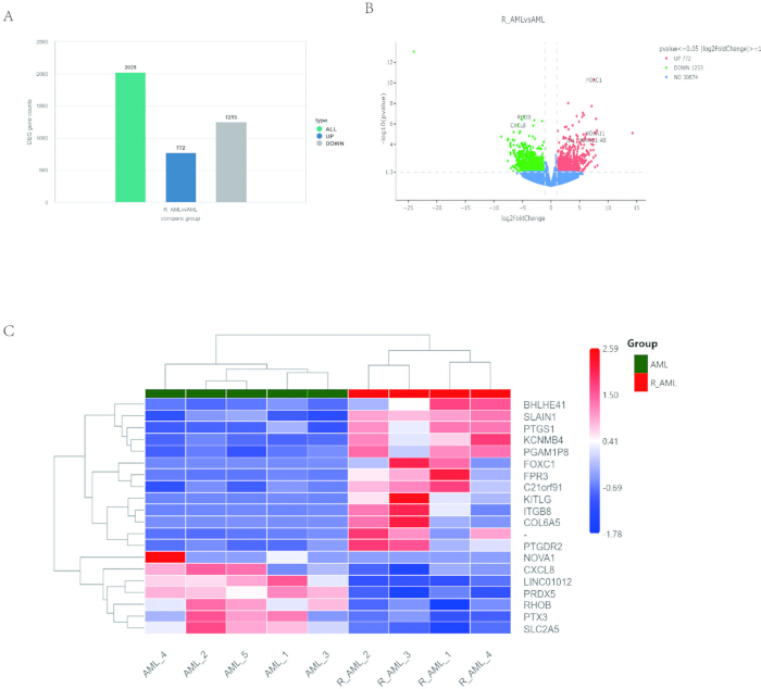
Figure 3: Differential gene expression analysis. (A) Bar plot showing the number of differentially expressed genes (DEGs) between comparison groups, identified by DESeq2 with thresholds of adjusted P-value ≤ 0.05 and |log₂FoldChange| ≥ 1. (B) Volcano plot of DEGs. The x-axis represents log₂FoldChange values, and the y-axis represents -log10(P-value). Blue dashed lines indicate the threshold lines used for DEG selection. (C) Hierarchical clustering heatmap of DEGs. The x-axis denotes sample names, and the y-axis shows normalized expression values of the DEGs. Please click here to view a larger version of this figure.

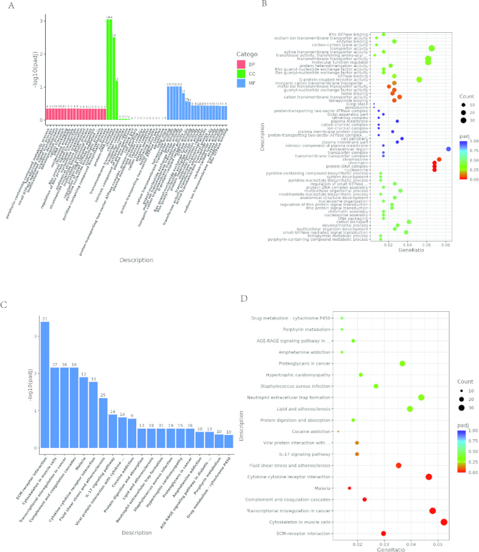
Figure 4: Functional enrichment analysis of differentially expressed genes. (A) GO enrichment bar plot. The x-axis represents GO terms, and the y-axis shows enrichment significance, expressed as -log10(padj). Colors represent BP (Biological Process), CC (Cellular Component), and MF (Molecular Function). (B) GO enrichment bubble plot. The x-axis represents the ratio of DEGs annotated to each GO term relative to the total number of DEGs, and the y-axis indicates the GO terms. Bubble size corresponds to the number of annotated genes, and color gradients represent enrichment significance. (C) KEGG enrichment bar plot. The x-axis represents KEGG pathways, and the y-axis denotes enrichment significance. (D) KEGG enrichment bubble plot. Bubble size indicates the number of annotated genes, and color gradients reflect enrichment significance. Please click here to view a larger version of this figure.

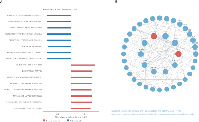
Figure 5: GSEA enrichment and protein–protein interaction (PPI) network analysis. (A) Bar plot showing normalized enrichment scores (NES) for selected significant gene sets. Positive NES values indicate enrichment in the R_AML group, whereas negative NES values indicate enrichment in the newly diagnosed AML group. (B) Protein–protein interaction (PPI) network. Each node represents a protein, and each edge denotes an interaction between connected proteins. Please click here to view a larger version of this figure.

Discussion

Critical Steps in the Protocol

The successful execution of this bioinformatic workflow relies on several critical steps. First, the immediate snap-freezing and proper lysis of the bone marrow aspirate (Step 1.6) are paramount, as the bone marrow microenvironment is rich in ribonucleases that can rapidly degrade transcriptomic integrity³⁰. During the computational phase, the correct configuration of the experimental design formula within the DESeq2 package (Step 6.3) is critical for accurate differential expression, particularly when clinical state (newly diagnosed versus relapsed) is contrasted while potential confounding variables are considered. Finally, applying rigorous false discovery rate (FDR) thresholds during Gene Set Enrichment Analysis (GSEA) (Step 9.6) is a critical statistical checkpoint to prevent the over-interpretation of false-positive functional networks.

Modifications and Troubleshooting

A common challenge in this method is the presence of batch effects, which frequently occur when clinical samples are collected and sequenced across extended timeframes. Batch variables should be defined before analysis, including sample collection date, RNA extraction date, library preparation batch, sequencing lane, and sequencing run. If PCA or sample correlation analysis reveals clustering based on sequencing date or another technical variable rather than clinical phenotype, users should modify the protocol by including the batch variable in the differential expression design formula when statistically feasible or by applying batch correction algorithms, such as ComBat or SVA, before visualization³¹. If applying this protocol to whole blood instead of bone marrow aspirates, an essential modification is the inclusion of a globin mRNA depletion step during library preparation to prevent highly abundant globin transcripts from monopolizing sequencing read depth. Software versions and principal parameters for the representative workflow were supplemented as follows: fastp v0.23.2, HISAT2 v2.0.5, StringTie v1.3.3b, featureCounts v1.5.0-p3, R v3.5.0, DESeq2 v1.20.0, clusterProfiler v3.8.1, org.Hs.eg.db v3.6.0, paired-end 150 bp sequencing, GSEA v4.2.3 with 1,000 gene-set permutations, MSigDB v7.5.1, STRING v11.5 with high-confidence interactions, and Cytoscape v3.9.1. Representative command-line parameters and analysis settings are provided in Supplementary File 1.

Limitations of the Method

While comprehensive, this protocol has inherent methodological limitations. First, it uses bulk RNA sequencing, which captures the average transcriptomic profile of the entire bone marrow aspirate and lacks single-cell spatial resolution. Therefore, the workflow cannot determine whether an upregulated relapse-associated signature originates from leukemia stem cells, stromal cells, immune cells, or changes in cell-type composition³². Second, the representative dataset is small (n = 9) and unpaired, which limits statistical robustness and prevents definitive causal inference. Third, the workflow is purely in silico. It generates candidate regulatory hubs and signaling pathways, but it cannot independently validate their functional necessity in chemoresistance without orthogonal in vitro or in vivo experimental validation.

Recent single-cell and single-cell genomic studies have expanded the AML reference framework by resolving cell-state heterogeneity, clonal architecture, and therapy-associated evolution at higher resolution^33,34,35,36. These approaches are complementary to the bulk RNA-seq workflow described here: bulk sequencing provides a practical and cost-effective screening strategy for cohort-level transcriptomic signatures, whereas single-cell and multi-omic methods can be used in follow-up studies to assign candidate signals to specific malignant or microenvironmental cell populations.

Significance with Respect to Existing Methods

Despite these limitations, this transcriptomic pipeline offers advantages over alternative diagnostic and analytical techniques. Traditional clinical assessments of AML relapse often rely on targeted multiplex qPCR panels or standard flow cytometry. While useful for rapid diagnostics, these targeted methods are constrained by predefined probes and can only evaluate known resistance markers¹⁹. By utilizing unbiased, genome-wide transcriptome sequencing paired with network analysis, this protocol can nominate novel transcripts and system-wide associations that existing targeted methods may overlook.

Importance and Potential Applications

The methodology outlined in this protocol is relevant to translational hematology and personalized medicine because it can prioritize transcriptomic signatures associated with relapse for additional study. A potential downstream application is the nomination of surface antigens or immune-evasion pathways that emerge during relapse. Such candidates could inform the design of future validation studies and, if experimentally confirmed, may contribute to the development of next-generation immunotherapies, including CAR-T or CAR-NK cell strategies³⁷. These translational applications should be considered hypothesis-generating rather than established conclusions from the present dataset.

Materials

List of materials used in this article

Name	Company	Catalog Number	Comments
Agilent 2100 Bioanalyzer	Agilent Technologies, Santa Clara, CA, USA	RRID:SCR_019389	G2939BA
AMPure XP system	Beckman Coulter, Brea, CA, USA	RRID:SCR_008452	A63881
cBot Cluster Generation System	Illumina, San Diego, CA, USA	-	SY-301-2002 or institution-specific system ID
clusterProfiler (Software)	Bioconductor	RRID:SCR_016884	v3.8.1
Cytoscape (Software)	Cytoscape Consortium	RRID:SCR_003032	v3.9.1
DESeq2 (Software)	Bioconductor	RRID:SCR_015687	v1.20.0
DNA Polymerase I	New England Biolabs (NEB, Ipswich, MA, USA	-	M0209L
dNTP Solution Mix	New England Biolabs (NEB, Ipswich, MA, USA	-	N0447L
edgeR (Software)	Bioconductor	RRID:SCR_012802	v3.22.5
fastp (Software)	OpenGene	RRID:SCR_016962	v0.23.2
featureCounts / Subread (Software)	The Walter and Eliza Hall Institute	RRID:SCR_012919	featureCounts v1.5.0-p3
GRCh38 reference genome	Genome Reference Consortium / Ensembl	-	GRCh38; Ensembl release 109
GSEA software	Broad Institute	RRID:SCR_003199	v4.2.3
HISAT2 (Software)	Johns Hopkins University	RRID:SCR_015530	v2.0.5
M-MuLV Reverse Transcriptase (RNase H-)	New England Biolabs (NEB, Ipswich, MA, USA	-	M0253L
MSigDB gene sets	Broad Institute	RRID:SCR_016863	v7.5.1
NEBNext Ultra II Directional RNA Library Prep Kit for Illumina	New England Biolabs (NEB, Ipswich, MA, USA	-	E7760L/E7765L or laboratory-specific kit
NEBNext Ultra II RNA Library Prep Kit for Illumina	New England Biolabs (NEB, Ipswich, MA, USA	-	E7770L
NovaSeq sequencing platform	Illumina, San Diego, CA, USA	RRID:SCR_016387	NovaSeq system; service-provider instrument ID
org.Hs.eg.db (Annotation package)	Bioconductor	-	v3.6.0
Phusion High-Fidelity DNA Polymerase	Thermo Fisher Scientific, Waltham, MA, USA	RRID:AB_2756816	F530L
Qubit 2.0 Fluorometer	Thermo Fisher Scientific, Waltham, MA, USA	RRID:SCR_018095	Q32866
Qubit dsDNA HS Assay Kit	Thermo Fisher Scientific, Waltham, MA, USA	-	Q32851
R software	R Foundation for Statistical Computing	RRID:SCR_001905	v3.5.0
Random Hexamer Primer	Thermo Fisher Scientific, Waltham, MA, USA	-	SO142
RNA 6000 Nano Kit	Agilent Technologies, Santa Clara, CA, USA	-	5067-1511
RNase H	New England Biolabs (NEB, Ipswich, MA, USA	-	M0297L
RNA-seq Library Prep Kit / Sequencing Service	Novogene, Beijing, China	-	Project No. X101SC25054246-Z01-J003
STRING database	STRING Consortium	RRID:SCR_005223	v11.5
StringTie (Software)	Johns Hopkins University / Center for Computational Biology	RRID:SCR_016323	v1.3.3b
TruSeq PE Cluster Kit v3-cBot-HS	Illumina, San Diego, CA, USA	-	PE-401-3001

References

- Döhner H, et al. Diagnosis and management of AML in adults: 2017 ELN recommendations from an international expert panel. Blood. 2017;129(4):424-47.
- Papaemmanuil E, et al. Genomic classification and prognosis in acute myeloid leukemia. N Engl J Med. 2016;374(23):2209-21.
- Arber DA, et al. The 2016 revision to the World Health Organization classification of myeloid neoplasms and acute leukemia. Blood. 2016;127(20):2391-405.
- Burnett AK, et al. Optimization of chemotherapy for younger patients with acute myeloid leukemia: results of the Medical Research Council AML15 trial. J Clin Oncol. 2013;31(27):3360-8.
- Ravandi F, et al. Phase I/II study of combination therapy with sorafenib, idarubicin, and cytarabine in younger patients with acute myeloid leukemia. J Clin Oncol. 2010;28(11):1856-62.
- Thol F, Schlenk RF, Heuser M, Ganser A. How I treat refractory and early relapsed acute myeloid leukemia. Blood. 2015;126(3):319-27.
- Zahreddine H, Borden KL. Mechanisms and insights into drug resistance in cancer. Nat Rev Drug Discov. 2013;12(4):314-28.
- Meads MB, Gatenby RA, Dalton WS. Environment-mediated drug resistance: a major contributor to minimal residual disease. Nat Rev Cancer. 2009;9(9):665-74.
- Ishikawa F, et al. Chemotherapy-resistant human AML stem cells home to and engraft within the bone-marrow endosteal region. Nat Biotechnol. 2007;25(11):1315-21.
- Pollyea DA, et al. Targeting acute myeloid leukemia stem cells: a review and principles for the development of clinical trials. Haematologica. 2014;99(8):1277-84.
- Shafat MS, Gnaneswaran B, Bowles KM, Rushworth SA. The bone marrow microenvironment-home of the leukemic blasts. Blood Rev. 2017;31(5):277-86.
- Lagadinou C, et al. BCL-2 inhibition targets oxidative phosphorylation and selectively eradicates quiescent human leukemia stem cells. Cell Stem Cell. 2013;12(3):329-41.
- Park IK, et al. Receptor tyrosine kinase Axl is required for resistance of leukemic cells to FLT3-targeted therapy in acute myeloid leukemia. Leukemia. 2015;29(12):2382-9.
- Ben-Batalla I, et al. Axl, a prognostic and therapeutic target in acute myeloid leukemia mediates paracrine crosstalk of leukemia cells with bone marrow stroma. Blood. 2013;122(14):2443-52.
- Farge T, et al. Chemotherapy-resistant human acute myeloid leukemia cells are not enriched for leukemic stem cells but require oxidative metabolism. Cancer Discov. 2017;7(7):716-35.
- Bosc C, et al. Mitochondrial inhibitors circumvent survival of leukemic stem cells. Cancer Cell. 2017;32(5):724-5.
- Li S, et al. Distinct evolution and dynamics of epigenetic and genetic heterogeneity in acute myeloid leukemia. Nat Med. 2016;22(7):792-9.
- Stevens AM, et al. Increased STAT3 activity in acute myeloid leukemia is driven by the bone marrow microenvironment. Cancer Res. 2017;77(18):5053-62.
- Wang Z, Gerstein M, Snyder M. RNA-Seq: a revolutionary tool for transcriptomics. Nat Rev Genet. 2009;10(1):57-63.
- Conesa A, et al. A survey of best practices for RNA-seq data analysis. Genome Biol. 2016;17(1):13.
- Chomczynski P, Sacchi N. Single-step method of RNA isolation by acid guanidinium thiocyanate-phenol-chloroform extraction. Anal Biochem. 1987;162(1):156-9.
- Love MI, Huber W, Anders S. Moderated estimation of fold change and dispersion for RNA-seq data with DESeq2. Genome Biol. 2014;15(12):550.
- Benjamini Y, Hochberg Y. Controlling the false discovery rate: a practical and powerful approach to multiple testing. J R Stat Soc Series B Stat Methodol. 1995;57(1):289-300.
- Yu G, Wang LG, Han Y, He QY. clusterProfiler: an R package for comparing biological themes among gene clusters. OMICS. 2012;16(5):284-7.
- Subramanian A, et al. Gene set enrichment analysis: a knowledge-based approach for interpreting genome-wide expression profiles. Proc Natl Acad Sci U S A. 2005;102(43):15545-50.
- Liberzon A, et al. Molecular signatures database (MSigDB) 3.0. Bioinformatics. 2011;27(12):1739-40.
- Szklarczyk D, et al. STRING v11: protein-protein association networks with increased coverage, supporting functional discovery in genome-wide experimental datasets. Nucleic Acids Res. 2019;47(D1):D607-13.
- Shannon P, et al. Cytoscape: a software environment for integrated models of biomolecular interaction networks. Genome Res. 2003;13(11):2498-504.
- Somerville TD, et al. Frequent derepression of the mesenchymal transcription factor gene FOXC1 in acute myeloid leukemia. Cancer Cell. 2015;28(3):329-42.
- Stark R, Grzelak M, Hadfield J. RNA sequencing: the teenage years. Nat Rev Genet. 2019;20(11):631-56.
- Leek JT, et al. The sva package for removing batch effects and other unwanted variation in high-throughput experiments. Bioinformatics. 2012;28(6):882-3.
- Hwang B, Lee JH, Bang D. Single-cell RNA sequencing technologies and bioinformatics pipelines. Exp Mol Med. 2018;50(8):1-14.
- Döhner H, et al. Diagnosis and management of AML in adults: 2022 recommendations from an international expert panel on behalf of the ELN. Blood. 2022;140(12):1345-77.
- Khoury JD, et al. The 5th edition of the World Health Organization classification of haematolymphoid tumours: myeloid and histiocytic/dendritic neoplasms. Leukemia. 2022;36(7):1703-19.
- Morita K, et al. Clonal evolution of acute myeloid leukemia revealed by high-throughput single-cell genomics. Nat Commun. 2020;11:5327.
- Miles LA, et al. Single-cell mutation analysis of clonal evolution in myeloid malignancies. Nature. 2020;587(7834):477-82.
- Kenderian SS, et al. CD33-specific chimeric antigen receptor T cells exhibit potent preclinical activity against human acute myeloid leukemia. Leukemia. 2015;29(8):1637-47.