A Semi-automated Method For Detecting Group Differences In Protocerebral Anterior Medial Cluster Dopaminergic Neuron Numbers In The Drosophila Brain

Summary

This protocol presents a semi-automated method for quantifying dopaminergic neuron numbers in the large Drosophila protocerebral anterior medial cluster. Designed specifically to detect and compare differences between experimental and control groups, this approach reduces reliance on manual counting and provides a practical tool for group-level analyses.

Abstract

Drosophila melanogaster serves as a powerful model organism for studying neurodegenerative diseases, including Parkinson's disease (PD), primarily through the analysis of dopaminergic (DA) neuron degeneration and associated locomotion deficits. Historically, quantification of DA neuron loss in the fly brain has been confined to smaller, readily countable clusters, including protocerebral posterior medial (PPM) clusters and protocerebral posterior lateral (PPL) clusters. In contrast, the substantially larger protocerebral anterior medial (PAM) cluster, comprising over 100 neurons, presents a significant challenge for manual counting, leading to its underrepresentation in quantitative studies. To date, reported investigations still rely on labor-intensive manual counts through confocal Z-stacks, which are time-consuming and prone to variability. To address this methodological gap, we developed a semi-automated image analysis pipeline using the open-source tool Labkit. This protocol enables efficient group-relative quantification of tyrosine hydroxylase (TH)-positive neurons in the PAM cluster within the same experimental batch. The method starts with standard immunofluorescence staining and confocal imaging, followed by a detailed, step-by-step guide for segmentation and analysis. This approach addresses the bottleneck of PAM cluster quantification and provides a practical workflow for detecting intergroup differences in DA neuron vulnerability in models of neurodegeneration. The relative scarcity of PD studies on the PAM cluster reflects a historical technical barrier rather than a lack of biological relevance. By overcoming this barrier, our method opens the door to systematic investigation of PAM neuron vulnerability in PD and its potential link to non-motor symptoms.

Introduction

The vinegar fly, Drosophila melanogaster, is a popular model organism for investigating the genetic and molecular underpinnings of neurodegenerative diseases, most notably Parkinson's disease (PD)¹. Its conserved neuronal signaling pathways, sophisticated genetic toolkit, and short lifespan make it exceptionally suited for studying age-dependent neuronal vulnerability and for conducting high-throughput genetic and pharmacological screens^2,3. Central to these investigations is the analysis of dopaminergic (DA) neurons, whose selective degeneration is a pathological hallmark of PD⁴. In the Drosophila brain, DA neurons are organized into discrete, genetically identifiable clusters^5,6. The progressive loss of DA neurons within specific clusters, visualized by TH immunostaining and quantified through microscopy, serves as a primary functional readout for assessing disease progression and neuroprotective interventions in experimental models^7,8. Thus, reliable quantification of DA neuron loss is essential for translating the power of Drosophila genetics into meaningful PD research outcomes.

Conventionally, quantitative analysis of DA neuron loss has focused on tyrosine hydroxylase (TH) immunostaining of small clusters, including protocerebral posterior medial (PPM) clusters and protocerebral posterior lateral (PPL) clusters, with each cluster containing fewer than 10 cells that are readily countable by eye⁷. Manual enumeration through confocal Z-stacks, while laborious, has been the established method for these clusters in many PD studies using Drosophila^9,10,11. In contrast, manual counting of the protocerebral anterior medial (PAM) cluster, the largest DA neuron group in the fly brain, comprising over 100 cells, presents a long-standing methodological bottleneck and precludes its inclusion in the majority of PD studies^9,10,11. Despite the critical role of PAM neurons in learning, memory, and motivation circuits, this limitation has resulted in their relative underrepresentation in quantitative analyses of neurodegeneration^12,13,14,15. Notably, even recent investigations continue to rely on this inefficient manual counting approach, underscoring a persistent and unmet need for a standardized, automated solution within the field¹³.

To address this critical gap, we have developed a semi-automated image analysis pipeline that enables efficient group-relative quantification of TH-positive (TH⁺) neurons in the PAM cluster within an experiment. This protocol leverages the open-source, machine learning-based plugin Labkit within the Fiji/ImageJ platform and 3D image processing software^16,17. The core workflow requires the user to annotate a representative subset of images to train a pixel classification model, which is then applied to batch-process experimental TH-staining datasets, followed by nucleus spot creation and classification relative to the TH⁺ region. This approach balances automation with expert oversight: it reduces the burden and variability of fully manual counts while retaining researcher input for guiding the algorithm and reviewing results.

The goal of this article is to provide researchers with a step-by-step protocol for efficient PAM cluster DA neuron relative quantification for group-relative comparisons within an experiment. We demonstrate the complete workflow, from brain dissection, immunofluorescence staining, and confocal imaging to the detailed image analysis pipeline using the semi-automated method. By standardizing this key quantitative step, this protocol aims to empower the research community to consistently incorporate the large PAM cluster into their analyses. This semi‑automated method is specifically designed for the PAM cluster and is not applicable to other dopaminergic clusters or to TH‑positive neurons in the optic lobes. This method may facilitate batch-level studies of PAM cluster DA neuron vulnerability and further investigations into synaptic plasticity, neurodegeneration, and therapeutic screening using the Drosophila model.

Protocol

1. Sample preparation and confocal imaging

1. Fly husbandry and collection
   1. Cross parent flies of the desired genotypes to generate experimental progeny. Upon eclosion, collect 20–30 flies per fresh food vial. Maintain flies according to the user's experimental design until the desired experimental age is reached.
2. Preparation for dissection
   1. Prepare a dissection dish by filling the lid of a 30 mm Petri dish to half‑height with Sylgard silicone elastomer. Fill the dish with 1x Phosphate-Buffered Saline (PBS). Aliquot 450 µL of fixative containing 1x PBS and 4% paraformaldehyde (PFA) in a 0.6 mL microcentrifuge tube, then place the tube on ice.
   2. Anesthetize 10–20 flies with a 5–10 s pulse of CO₂, then immediately transfer them onto a 60 mm Petri dish placed on ice to maintain immobility.
      CAUTION: PFA is toxic and a suspected carcinogen. Handle in a fume hood with gloves, lab coat, and safety goggles. Dispose of waste per institutional hazardous material guidelines.
3. Fly brain dissection and fixation
   1. Grasp a fly by the wing root using forceps and immerse it ventral side up into the PBS-filled dissection dish. Pierce the thorax with a fine dissection pin to anchor the fly on the Sylgard pad.
   2. Orient the body horizontally (e.g., head left, abdomen right). Hold the proboscis base with one forceps while using the other to remove the entire proboscis, creating an opening between the compound eyes.
   3. Grasp the exposed eye edges with two forceps and very slowly pull them apart symmetrically, exposing the brain while preserving its connection to the ventral nerve cord.
   4. Remove the tracheal sacs and fat body surrounding the brain. Sever the ventral nerve cord to free the brain and allow it to settle on the dish with its anterior side facing upward.
      NOTE: If the settled brain shows the ventral half positioned higher than the dorsal half (Figure 1B,C), use forceps to gently press down the raised portion.
   5. Prewet a P10 pipette tip with 0.1% Triton X-100 to prevent the dissected brain from adhering to the inner wall of the tip. Using this prewetted tip, transfer each dissected brain into the tube containing fixative, then proceed to the next dissection. After all brains have been transferred, invert the tube 5x and place it horizontally on ice for 30 min. Incubate the tube at room temperature (RT) for 1 h with agitation.
   6. Allow brains to settle to the bottom for 1 min. Wash the brains for 3 x 10 min with washing solution containing 1x PBS and 0.1% Triton X-100 (PBST) with agitation. Store the brains in PBS containing 0.1% sodium azide at 4 °C or proceed to immunostaining.
4. Immunostaining
   1. Stain brains in 300 µL of primary antibody staining solution containing 1x PBS, 0.1% Triton X‑100, 5% Normal Goat Serum, 0.1% Sodium azide, and rabbit anti-TH antibody (1:500 dilution) for 2 days at 4 °C with agitation. Wash the brains for 3 x 10 min with PBST.
   2. Stain the brains in secondary antibody solution containing 1x PBS, 0.1% Triton X‑100, 5% Normal Goat Serum, 0.1% Sodium azide, and anti‑rabbit Alexa Fluor 635 for 2 days at 4 °C. Wash the brains once with PBST.
   3. Incubate brains in PBST supplemented with 4’,6-diamidino-2-phenylindole (DAPI) (1:1,000 dilution) for 2 h at RT, then wash the brains in PBST for 2 h. Store brains at 4 °C overnight or proceed to mounting.
5. Mounting
   1. Load 0.5 mL of mountant to a 1 mL syringe fitted with a fine-gauge needle. Create a mounting chamber by affixing two parallel strips of transparent adhesive tape onto a glass slide, leaving a 3 mm gap (Figure 1A,D).
      CAUTION: Sharp needles pose a puncture hazard. Always handle with care, recap using a one-handed scoop technique if necessary, and dispose of used needles immediately in an approved sharps container.
   2. Transfer brains into a clean Petri dish using a truncated P200 tip. Remove excess liquid surrounding brains and dispense 10 µL of mountant onto the brains. Gently mix the brains with the mountant.
   3. Dispense three droplets of mountant along the gap on the slide and spread evenly across the gap. Transfer and position the brains along the central line of the gap with a P10 pipette (Figure 1A).
   4. Position brains evenly along the centerline of the gap with the anterior side facing upward. Slowly cover the gap with a coverslip. Press down near the edges of the coverslip with thumbs for 3 s to ensure firm contact.
   5. Place the slide horizontally in a slide folder to cure overnight at RT in the dark, then at 4 °C for long-term storage.
6. Confocal imaging
   1. Power on the confocal microscope system and wait for 15 min for laser stabilization. Locate the brains in bright field with a 10x objective lens, then switch to a 100x oil immersion objective lens and navigate to the PAM cluster under live view.
   2. Adjust stage XY to locate one PAM cluster in the imaging center. Preview through Z to confirm the boundaries and orientation. Adjust the digital zoom and orientation until the PAM cluster fits the imaging frame along the diagonal.
   3. Set the top and bottom position of the stack. Set the Z-step size to 0.34 µm and image resolution to 512 x 512. Set the pin hole to auto mode. Set the display lookup table (LUT) to saturation indicator.
   4. Adjust the laser power and detector gain of the TH channel until a minimum amount of scattered, discrete puncta within PAM neurons is saturated. Adjust the settings of the DAPI channel to obtain a bright, clear nuclear signal without saturation.
      NOTE: The optimal zoom factor varies. Differences in tissue shrinkage can occur between experimental batches and among individual brains within the same batch.
   5. Acquire and save images in raw format with 12-bit or 16-bit in the input folder (e.g., D:\Confocal\images). Return to live view, reset zoom, and browse along the gap to find the next brain without switching to lower magnification.
      NOTE: Do not save, export, or convert the primary data files into a processed .tif format at this stage. Preserving the original raw metadata is essential for subsequent image processing.

2. Image processing and quantification

1. Image file conversion and TH channel split
   1. Convert raw images located in the input folder to a format compatible with the 3D image analysis software using the associated file converter (Table of Materials). Place the converted files in the converted folder (e.g., D:\Confocal\converted)
   2. Open Fiji and navigate to File | New | Script. In the script editor, click File | Open to load macro file ImageFolder_Split_ChannelAndSaveMacro_UltimateDepth.ijm (Supplemental File 1). Click Run near the bottom of the editor window (if the button is hidden, click the small triangular icon to show it).
   3. In the configuration dialog, click Browse and select the converted folder. Under Naming Convention, select option 3. Under Channel to export, select the channel index corresponding to TH. Click OK to batch-split the TH channel; the exported TH stacks will be saved automatically in a folder ending with ChannelSplitOut.
2. Training the Labkit classifier
   1. Preparation of the training dataset
      1. Select 20 representative stacks that capture a range of signal intensities and background variations of samples from the TH stack folder. Copy the selected files to the selection folder (e.g., D:\Confocal\selection).
      2. Run the Fiji macro ImageFolder_UniCropZStack_ToThinestLayers.ijm (Supplemental File 2). When prompted, select the folder containing the training images. The macro trims each stack to the same number of Z-slices and concatenates the stacks into a time-lapse TIFF file for training.
   2. Interactive training of pixel classifier
      1. Launch Labkit via Fiji Plugins | Labkit | Open Current Image With Labkit (Table of Materials). In the toolbar, click the 3D Box button to switch to Slice View mode for navigation through Z‑slices (slider on right side) and across samples (slider on bottom).
      2. Press S to open the Brightness and Contrast panel and adjust the Max slider for optimal visualization of TH⁺ neurons. Set an appropriate brush size (e.g., 5 pixels). Click Settings to expand the tool panel. Keep the default Display Modes (Fused, Source, Nearest).
      3. Click Draw. In the Labeling panel, highlight Background and draw on a few non‑cellular regions; highlight Foreground and draw on the interior of a few TH⁺ neurons.
      4. Zoom in and out of the field with Ctrl + Shift + Scroll. Navigate to other Z‑slices using the vertical slider and to other training samples using the bottom slider. Repeat drawing several times to ensure robust classifier training.
      5. Click the Pixel Classification. Click the Start Training triangle to initiate training and lazy prediction, which later provides real‑time segmentation feedback while navigating across samples, slices, or positions (right-click and drag) anytime.
      6. Click Draw to add corrective annotations where prediction is inaccurate, with optional toggling of the visibility of prediction and label in the Sources panel and re-train. Iterate until the classifier reliably distinguishes TH⁺ neurons from background, then save the classifier via Segmentation | Save Classifier before closing Labkit.
3. Batch Labkit segmentation
   1. Open a random image from TH stack folder in Fiji. Launch Labkit and click Remove All, then load the pretrained classifier via Segmentation | Open Classifier to segment the image. Visually inspect the quality to validate classifier generalizability, then close the window.
   2. Repeat 2.3.1 on several other random images. Close the window after each inspection except the final one.
   3. Create a Labkit output folder (e.g., D:\Confocal\LabkitOut). Start batch processing via Others > Batch Segment Images. Set Input Directory to the TH stack folder and set Output Directory to the Labkit output folder, and then click OK to start batch processing.
   4. For future experiments using the same TH antibody and comparable confocal settings, skip 2.2 and re-use the previous classifier.
      NOTE: We also provide a pretrained classifier for testing purposes (Supplemental File 3).
4. DAPI spot creation and TH⁺ neuron quantification
   1. Place XT_Jove_Labkit_TH.m (Supplemental File 4) in a script folder (e.g., D:\scripts). Open 3D software and navigate to File | Preferences, then select Custom Tools. On the XTension Folder panel, click Add… to select script folder and click OK.
   2. For each converted file, the script will automatically execute the following sequential operations.
      ​NOTE: This explanatory section does not contain actions for the user but is essential for proceeding to the next steps.
      1. The DAPI channel is processed by Background Subtraction and Gaussian Filter to facilitate optimized DAPI spot identification.
      2. The Labkit segmentation mask is refined by denoising and hole‑filling and attached as a mask channel to the dataset. A refined TH surface object is constructed from the mask channel. The TH surface object further generates a refined mask to overwrite the mask channel.
      3. A distance transform channel is created from the TH surface, where voxels inside the surface are set to 0 and voxels outside the surface are assigned with floating‑point values representing their Euclidean distance to the nearest TH surface.
      4. Use the intensity profile of each DAPI spot in the distance transform channel as a metric for TH⁺ neuron identification. DAPI spots located within or close to TH⁺ regions have low distance values. This criterion helps rescue false negatives, such as real DA neuron nuclei located just outside but immediately adjacent to an imperfect Labkit-predicted foreground region.
   3. Manual optimization of Quality for DAPI spot creation
      1. Open a random sample from the converted folder in 3D software. Navigate to Edit | Image Properties and verify whether the Voxel Size Z in the Coordinates panel is 0.340 µm. If not, manually change it to 0.340 µm.
      2. Apply background subtraction to the DAPI channel by clicking Image Processing | Thresholding | Background Subtraction. In the dialog, tick only the DAPI channel, set Filter Width to 3, and click OK. Repeat this step once more and then perform a third repeat with a filter width of 1.
      3. Apply Gaussian smoothing by clicking Image Processing | Smoothing | Gaussian Filter. Tick only the DAPI channel, set Filter Width to 0.2, and click OK.
      4. In the Surpass Scene, click Add New Spots to launch the Spots creation wizard. Select the DAPI channel and enter an Estimated XY Diameter of 1.2 µm. Following the wizard, add a "Quality above" filter and finetune the threshold until it robustly yields an accurate single spot for each nucleus.
      5. Repeat steps 2.4.3.1–2.4.3.4 across several random selected samples, and finalize threshold value(s) that work reliably across samples.
   4. Open the script XT_Jove_Labkit_TH.m (Supplemental File 4) in the text editor to modify the following user‑defined parameters.
      1. Set ims_Folder to the path of the converted folder; set LabkitOut_Folder to the path of the Labkit output folder. Set Ch_DAPI to the DAPI channel index for all files in the converted folder (e.g., 1 if DAPI is the first channel, 2 if DAPI is the second channel).
      2. Set reVoxelSizeX, reVoxelSizeY, reVoxelSizeZ. If voxel sizes are correct in Image Properties (see step 2.4.3.1), leave the answers as empty brackets []. Otherwise, manually enter suitable values (e.g., 0.130, 0.130, 0.340, respectively) which will be applied to all files in converted folder.
   5. Finalize the spot creation parameters.
      1. Customize multiple versions of parameters in the SpotsParameterAss cell array, where each row specifies one version. This includes defining Estimated XY diameter (µm) for DAPI spot detection in the left part of each row, and defining Filter String composed of criteria filter(s) in the right part of each row, containing the Quality threshold(s) from step 2.4.3.4 and/or Intensity thresholding on the refined mask channel from step 2.4.2.2 or distance transformed channel from step 2.4.2.3.
      2. Set "Intensity Center Ch=aSizeC+1" above 0.5 to retain only spots whose geometric center falls within the refined TH mask channel from 2.4.2.2 (voxel value > 0.5). This is the most direct and stringent criterion for TH⁺ DAPI spot filtering.
      3. Set “Intensity Mean Ch=aSizeC+2” below [threshold] to retain spots whose average intensity in the distance transform channel from step 2.4.2.3 falls below a specified threshold. Lower thresholds select spots positioned inside or extremely close to the TH surface; higher thresholds include spots progressively farther away. This allows empirical calibration of the acceptable proximity for TH⁺ assignment.
      4. Preconfigured example:
         SpotsParameterAss = {
         1.2, ['"Quality" above 94.5,"Intensity Center Ch=aSizeC+1" above 0.5'];
         1.2, ['"Quality" above 94.5,"Intensity Mean Ch=aSizeC+2" below 0.0001'];
         1.2, ['"Quality" above 94.5,"Intensity Mean Ch=aSizeC+2" below 0.001'];
         1.2, ['"Quality" above 94.5,"Intensity Mean Ch=aSizeC+2" below 0.01'];
         ... more combinations of filter are provided in script.
         };
      5. For future experiments using the same TH antibody and confocal settings, re-use the previous parameter combinations. Delete those poor combinations that yield spot counts deviating substantially from the actual numbers, thereby reducing unnecessary computational burden.
   6. Batch spot creation
      1. Save all above modifications to the script XT_Jove_Labkit_TH.m. Open a new 3D software window. Click menu Image Processing | PAM_TH_processing to execute the script in batch.
      2. Initially, observe for a few minutes that for each filter combination, the script creates a Spots object named to reflect its parameters, and that files from the converted folder are processed and saved as copies in a new output folder suffixed with "processed". Then leave the computer unattended.
      3. Upon completion, a spreadsheet will be generated. Observe the first column containing file names, and subsequent columns containing DAPI spots counts corresponding to each filter combination, with column headers indicating the Estimated XY diameter and Filter String used.
   7. Postprocessing validation
      1. After step 2.4.6 completes, manually open a few random files from the "processed" folder and examine the different Spots objects in overlay with the original TH channel. Based on visual inspection, select one or two optimal filters that yield the most faithful representation of true TH⁺ neuron counts. Export the corresponding columns from the spreadsheet for downstream statistical analysis and figure preparation.
      2. To correct spot-count errors in the preferred filter combination(s), select the corresponding Spots object(s) in the Surpass scene and click the Edit tab. Manually remove erroneous spots or add missed spots as needed by pressing Shift and clicking on the screen. Save the updates using Store as/Export as/Save as to overwrite the corresponding file in the "processed" folder with the same file name.
         NOTE: Do not delete, add, rename, or drag/reposition any Spots objects—only edit the spots preferred. No modifications to the script are required; simply re‑run the script to instantly generate an updated spreadsheet reflecting manual refinements. For consistency, either leave none edited, or edit the preferred Spots object(s) for all samples in an experiment.

Results

The raw data collected from the software have been deposited in a public repository and are accessible at the following DOI: 10.5281/zenodo.19814348. To demonstrate the use of this semi-automated quantification pipeline, we applied it to a well-established Drosophila model of PD using pan-neuronal expression of human α-synuclein (nSyb-QF2>QUAS-SNCA). Control flies harbored the nSyb‑QF2 driver alone. Both genotypes were aged at 29 °C for 3 weeks, after which brains were dissected, immunostained for TH, and imaged for the PAM cluster. As shown in Figure 3E, the semi-automated pipeline detected a significant reduction in PAM TH⁺ neuron counts in α-synuclein-expressing flies compared to controls (Student’s t-test, p < 0.0001), demonstrating that the method can capture genotype-dependent differences within the same experimental batch. The following sections describe the mounting configuration (Figure 1), the Labkit training interface (Figure 2), and the image processing steps (Figure 3) that enable this quantification.

Figure 1 illustrates the mounting configuration of dissected Drosophila brains and its impact on PAM cluster imaging. After dissection, brains occasionally exhibit bending or tilting-up of the tissue adjacent to the severed ventral nerve cord. This lifting at the ventral part of the brain alters the perspective under the stereoscope, leading to altered projection of the stereotypic furrow in the dorsal contour and a difference in the relative perspective of ventral landmarks. (Figure 1B,C). This deformation often occurs at the moment the brain is detached from the body. Such deformation affects the orientation of the PAM cluster during mounting, consequently influencing the required Z-stack depth (Figure 1C,D). Under optimal mounting conditions, the single-layer Scotch tape spacer creates an adequate compression on the central brain region, causing the dorsally located PAM cluster to assume a horizontal orientation immediately adjacent to the coverslip. This configuration yields Z-stacks of 15–25 slices at 0.34 µm intervals (Figure 1D). In the other condition, the PAM cluster retains a tilted position, necessitating deeper Z-stacks (Figure 1D). Similarly, use of a double-layer tape spacer fails to provide adequate compression, leaving the PAM cluster in its native, tilted conformation and likewise increasing Z-stack depth (Figure 1D). Figure 1E shows representative lateral projection views of TH-stained Z-stacks under both optimally positioned and tilted conditions.

Figure 2 presents the Labkit user interface and a representative training workflow. With only a few sparse scribble annotations on a single sample (Figure 2A), the initial pixel classifier already produces a remarkably reasonable segmentation (Figure 2B). However, it is critical to emphasize that such minimal annotation is insufficient for robust, generalizable performance across an entire dataset. Substantially more iterative labeling—spanning multiple Z-slices, samples, and staining variations—is required to generate a classifier that reliably segments TH⁺ neurons across the full dataset. Notably, the multiple training images are concatenated along the time (frame) dimension rather than stacked along the Z-axis. This design preserves the spatial integrity of each individual brain volume, ensuring that 3D filter kernels operate exclusively within—not across—biological specimens. If samples were instead stacked vertically into a single thick Z-stack, Z-slices at the boundaries between adjacent samples would become spatially contiguous, causing voxels from different brains to be treated as neighboring structures, which would increase the risk of unnecessary manual corrections (Figure 2C). Concatenation along the time axis avoids such cross-sample contamination while still enabling efficient, multi-sample training in a single Labkit session.

Figure 3 illustrates the post-processing pipeline and final quantification. Raw Labkit segmentation masks (Figure 3A) contain numerous small false-positive speckles and internal holes. After applying morphological denoising and hole-filling operations (Figure 3B), a smoothed TH surface is constructed and used to generate a refined binary mask (Figure 3C). The improvement achieved by this refinement is visualized as an overlay comparing the initial and final masks (Figure 3D, upper). Notably, some TH-rich neurite regions are occasionally retained in the final mask; however, these areas are almost invariably devoid of DAPI-stained nuclei and therefore contribute negligibly to final neuron counts. Advanced users may further adjust the morphological parameters in the provided batch-processing script to fine-tune the elimination of such residual artifacts. Figure 3D (lower) shows the final DAPI spots (magenta) overlaid on the TH channel (green) from a maximum intensity projection. Figure 3D also reveals a rare type of false positive occasionally observed in our pipeline: a DAPI‑stained nucleus located within a TH‑rich neurite region may be incorrectly classified as a TH⁺ spot when the neurite signal strongly overlaps with the nucleus. However, as shown in Figure 3C, DAPI‑positive nuclei in the vicinity of neurites are generally sparse. Moreover, the few DAPI signals present near such neurite regions often remain correctly classified as true negatives (i.e., not counted as TH⁺), as they are not misidentified by the pipeline. Figure 3E demonstrates the practical utility of the method: 3-week-old nSyb-QF2>SNCA flies exhibit a significant reduction in PAM TH⁺ neuron counts compared to nSyb-QF2 controls across multiple filters (Student's t-test, p < 0.0001). Although the absolute spot counts may vary across different filter combinations and the method does not achieve perfect single-spot accuracy, the relative difference between experimental and control groups remains robust. For multiple filters tested, the statistical outcome of group comparison is largely preserved across filters within the same experimental batch. Accordingly, the output should be interpreted as a within-batch comparative readout rather than an error-free absolute count of PAM neurons.

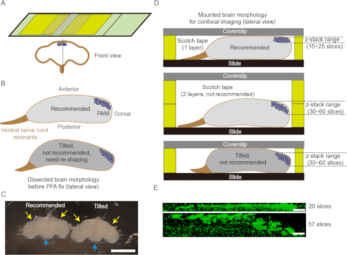
Figure 1. Drosophila brain dissection and mounting configuration. (A) Schematic diagram of the brain mounting assembly. Yellow bars represent Scotch tape spacers. An enlarged brain schematic indicates the approximate location of the PAM cluster (purple). (B) Lateral cross-sectional schematics corresponding to the dashed plane in A depicting two common brain morphologies after dissection: optimally positioned (upper) and tilted (lower). (C) Two dissected fly brains viewed under a stereoscope: optimally positioned (left) versus tilted (right). Yellow arrows indicate the stereotypic furrow along the dorsal contour. Blue dashed lines connect two corresponding landmarks on the left and right sides of the ventral half. Blue arrows highlight the resulting shift in the relative perspective of these ventral landmarks. Scale bar = 500 µm. (D) Schematic illustration showing how brain morphology and tape spacer thickness (single- vs. double-layer) influence the vertical positioning of the PAM cluster and consequently the required Z-stack depth. (E) Representative lateral views (Y projection) of TH-stained confocal Z-stacks from optimally positioned (upper) and deformed (lower) mounting conditions. Scale bar = 5 µm. Abbreviation: PAM = protocerebral anterior medial. Please click here to view a larger version of this figure.

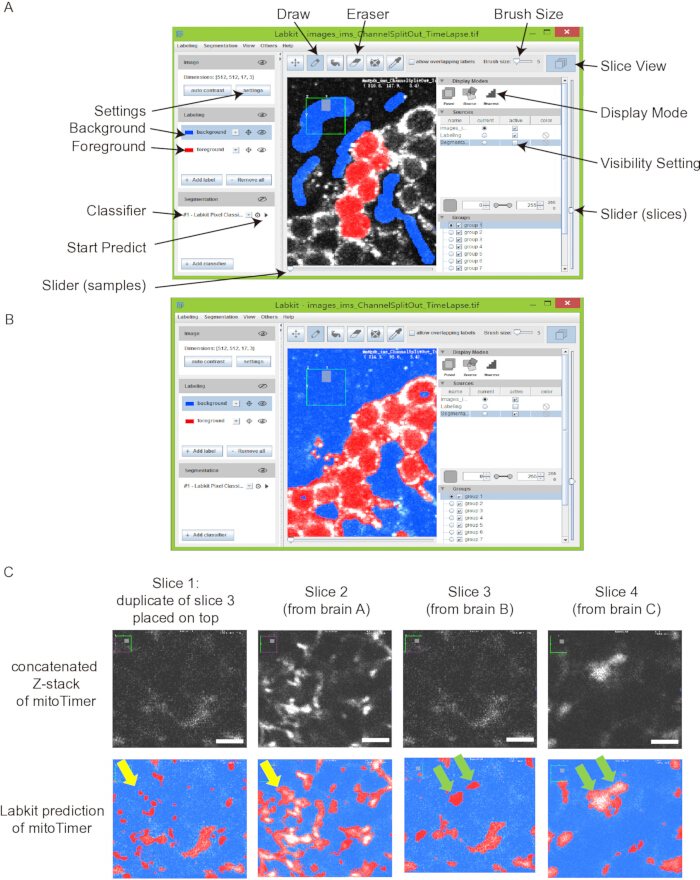
Figure 2. Labkit training and interactive segmentation. (A) Labkit graphical user interface. Annotations (scribbles) are shown in two classes: foreground (red) and background (blue). (B) Segmentation result generated immediately after training on the scribbles shown in A. Red indicates foreground color; blue indicates background color. Scale bar = 5 µm. (C) Cross-talk between adjacent Z-slices. Single-slice images of fluorescent protein-labeled mitochondria from different fly brains were concatenated along the Z-axis. Slices 1 and 3 are identical copies of the same image, while slices 2 and 4 originate from different brains. Yellow arrows, prediction bleed-through from slice 2 into slice 1. Green arrows, prediction bleed-through from slice 4 into slice 3. Scale bar = 3 µm. Please click here to view a larger version of this figure.

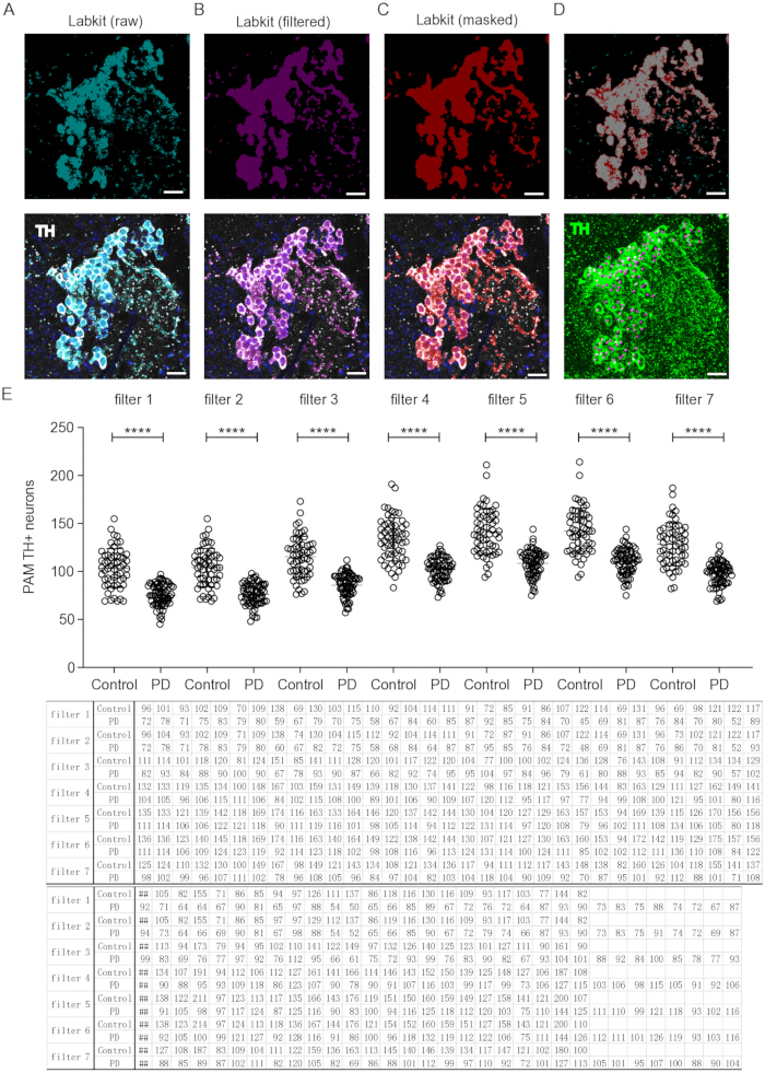
Figure 3. Postprocessing of Labkit segmentation masks and TH⁺ neuron quantification. (A) Raw Labkit binary mask (cyan, upper) and overlay with the original TH channel (lower). Note abundant small speckles and incomplete filling of neuronal cell bodies. (B) Mask after morphological denoising and hole-filling (magenta, upper); overlay with TH channel (lower). (C) Refined binary mask (red, upper) from a smoothed TH surface for B and re-masking; overlay with TH channel (lower). (D) Upper: Overlay of raw (cyan) and refined (red) masks, highlighting regions corrected by post-processing. Lower: Maximum intensity projection showing final DAPI spots (magenta) superimposed on the TH channel (green). Note that the two spots on the upper-right corner originate from the contralateral PAM cluster. Filter 4 was used for illustration. (E) Quantitative validation in a Parkinson's disease model using multiple filter combinations. Three-week-old nSyb-QF2>SNCA (PD model) flies exhibit a significant reduction in PAM TH⁺ neuron counts compared to nSyb-QF2 controls in multiple filters (top). Raw data is provided in a spreadsheet (bottom). filter 1: 1.2, ['"Quality" above 94.5,"Intensity Mean Ch=aSizeC+2" below 0.0001']; filter 2: 1.2, ['"Quality" above 94.5, "Intensity Mean Ch=aSizeC+2" below 0.001']; filter 3: 1.2, ['"Quality" above 94.5,"Intensity Mean Ch=aSizeC+2" below 0.01']; filter 4: 1.2, ['"Quality" above 94.5,"Intensity Mean Ch=aSizeC+2" below 0.05']; filter 5: 0.6, ['"Quality" above 94.5,"Intensity Mean Ch=aSizeC+2" below 0.001']; filter 6: 0.6, ['"Quality" above 94.5,"Intensity Mean Ch=aSizeC+2" below 0.01']; filter 7: 0.9, ['"Quality" above 94.5,"Intensity Mean Ch=aSizeC+2" below 0.01']; n = 57 brains (control), n = 65 brains (PD); Student's t-test, p < 0.0001 (****). Flies were cultured at 29 °C. Scale bars = 5 µm (A–D). Data are presented as mean ± SD. Please click here to view a larger version of this figure.

Supplemental File 1. Fiji macro for splitting the TH channel from converted image files and saving the output stacks.Please click here to download this file.

Supplemental File 2. Fiji macro for cropping training Z-stacks to a common Z-slice depth and concatenating them into a time-lapse TIFF file for Labkit classifier training.Please click here to download this file.

Supplemental File 3. Pretrained Labkit classifier used for testing the PAM TH segmentation workflow.Please click here to download this file.

Supplemental File 4. MATLAB script for batch processing Labkit masks, generating DAPI spots, applying filter combinations, and exporting TH⁺ neuron counts.Please click here to download this file.

Discussion

Quantification of DA neurons in the Drosophila PAM cluster has historically been a formidable challenge. Here, we present a semi-automated workflow that integrates machine learning-based pixel classification with image analysis software to address this long-standing issue. This method enables batch-level detection of variations in TH⁺ neurons in the PAM cluster among groups within the same experiment, supporting comparative studies in Parkinson's disease models¹⁸.

When selecting the optimal filter for a given experiment, users may either choose the filter that best matches visual inspection of the raw images, or refer to the reported range and/or average of wild‑type PAM neuron numbers in the literature^12,13. However, caution is warranted: only two studies have reported PAM cluster counts, neither of which is PD‑related, and the reported values show considerable inconsistency. Moreover, the standard deviation may increase with age, further complicating cross‑study comparisons. Therefore, literature‑based reference should be used only as a rough guide, not as an absolute standard. We acknowledge that this pipeline does not yield error‑free absolute counts (Figure 3D). However, as long as comparisons are confined to groups within the same experimental batch (i.e., not pooling data across different batches in a single plot), the method can be used to detect relative differences between genotypes or treatment conditions within a batch.

In our experience, AF488‑conjugated secondary antibodies should be avoided due to high background, and AF546 should be avoided due to higher signal attenuation along the Z‑axis. We also found that thorough DAPI incubation and washing are critical for achieving high signal‑to‑noise ratio and clear nuclear signals, which directly impact the performance of automated segmentation. DAPI is preferable to Hoechst for this application, as its preferential staining of heterochromatin generates brighter and more sharply defined nuclear spots, facilitating more accurate detection.

Troubleshooting discussion for common failure modes

Staining‑related failures. Dissection skill is a major determinant of data quality. The PAM cluster is located superficially and is easily damaged when removing the two tracheal sacs and fat body dorsal to this region. Forceps should be handled with care to avoid piercing or compressing the PAM area. Ventral deformation often occurs at the moment the ventral nerve cord is severed, causing the brain to tilt or curl when placed on a glass slide; this deformation can become permanently fixed after PFA incubation. Users should experiment with forceps angles during severing to find an optimal technique. If tilting is observed post‑dissection, gentle pressure on the elevated region may reverse the deformation (acceptable if the compressed area is not the region of interest).

Segmentation failures. Poor segmentation usually arises from insufficiently diverse training data. The Labkit classifier must be trained on a representative set of images spanning the full range of staining quality within the batch, including best, average, and poorest. During iterative correction, prioritize annotating false positives and false negatives that you are confident about. Avoid correcting ambiguous or uncertain regions, as this may mislead the classifier and degrade performance.

Spot detection failures. Parameter optimization requires systematic exploration on a small subset of representative samples. Test different estimated spot diameters and Quality filter threshold, or even filter types beyond the "Quality above" filter used in this protocol. The spot creation wizard offers various filtering options (e.g., intensity). Users are encouraged to adapt filter thresholds and types to their specific dataset, and to perform empirical tuning before batch processing.

Why does manual counting of PAM cluster neurons remain exceptionally difficult? The PAM cluster presents unique anatomical and staining characteristics that render traditional manual counting methods inadequate. First, TH immunofluorescence in the cytosol of Drosophila dopaminergic neurons predominantly labels a thin cytoplasmic ring surrounding a large, unstained nuclear void. Consequently, the DAPI-stained nucleus and the TH⁺ cytoplasmic compartment exhibit minimal spatial overlap. This fundamental lack of colocalization precludes the direct "DAPI spot within TH mask" classification strategy. Second, the PAM cluster comprises over 100 densely packed neurons arranged in a three-dimensional, grape-like architecture. As one navigates through confocal Z-stacks, neurons gradually appear and disappear—some entering the plane, others exiting—creating a high cognitive load and substantial inter-observer variability. The most recent study quantifying PAM DA neurons relied on manual counting using ImageJ's cell-counter plugin. While entirely appropriate for smaller clusters such as PPM1/2 or PPL1, this approach becomes prohibitively labor-intensive when applied to the PAM cluster, particularly in studies requiring dozens or hundreds of samples.

Why is Labkit’s random forest architecture particularly well-suited for TH neuron segmentation? Labkit implements a random forest-based pixel classifier that is exceptionally well adapted to the specific challenges of TH-stained PAM cluster images. The algorithm computes a comprehensive feature vector for each pixel by applying a cascade of transformation filters, including Gaussian blur, difference of Gaussians, Gaussian gradient magnitude, Laplacian of Gaussian, and Hessian eigenvalues—each evaluated at multiple sigma scales (1, 2, 4, 8). This multi-scale feature extraction effectively captures the textural and edge characteristics that distinguish the nuclear interior from the extracellular background. Importantly, because random forests require orders of magnitude less training data than deep learning approaches, users can iteratively refine the classifier with sparse scribble annotations on as few as 20–40 representative images. Each iteration adds new decision trees to the ensemble, which collectively vote to classify each pixel. This process inherently accommodates batch-to-batch variability in staining and imaging conditions—a critical advantage given the biological variability inherent in Drosophila genetic crosses and aging studies. Using this approach, TH⁺ neuron loss in α-synuclein-expressing Parkinson's models can be detected, and the effects of genetic enhancers and suppressors on PAM cluster neuron counts can be compared within an experimental batch.

Importantly, for the purpose of training, the cropped stacks are concatenated along the time dimension rather than stacked along the Z-axis. This design choice is critical for optimal classifier training. Labkit's 3D pixel classification considers voxel information across consecutive Z-slices, which is essential for accurately resolving the thin, cytoplasmic TH ring that defines PAM neuron morphology. If the individual samples were instead stacked vertically into a single, ultra-thick Z-stack, the Z-slices at the boundaries between adjacent samples would become spatially contiguous in the stack. Consequently, voxels belonging to different biological samples would be treated as neighboring structures within the same three-dimensional volume. During interactive training, a scribble drawn near such a boundary may inadvertently capture features from two different samples simultaneously, confusing the classifier (Figure 2B, arrows). Moreover, false-positive signals originating from one sample could project into the adjacent sample's volume, resulting in erroneous corrective scribbles which propagate through subsequent training iterations, generating decision trees that encode biologically meaningless rules. Concatenating samples along the time axis preserves the spatial integrity of each individual volume, allowing the 3D filter kernels to operate exclusively within—not across—biological specimens, while still enabling efficient, multi-sample training in a single Labkit session.

Methodological considerations and limitations

Several important caveats merit discussion. First, this protocol is optimized specifically for the PAM cluster and may not generalize to other DA clusters (e.g., PPM1/2/3, PPL1) or to TH⁺ neurons in the optic lobes. The PAM region benefits from relatively sparse DAPI density, with nuclei well-separated in three-dimensional space, enabling robust and unambiguous DAPI spot detection. In contrast, this workflow is not readily transferable to other DA clusters such as PPL1 or PPM1/2. In those regions, neurites are more likely to be juxtaposed with or overlap DAPI‑stained nuclei of non‑DA cells. Given the very low baseline number of DA neurons in these small clusters (often fewer than 10 cells per cluster), even a few misclassifications can lead to proportionally large errors, making the method less reliable for such applications. Second, TH immunostaining also labels neurites and axonal projections within the neuropil. Despite corrective annotations during training, these fiber tracts occasionally produce strong TH signals and may be misclassified as foreground by the classifier. However, these regions in PAM cluster are almost invariably devoid of DAPI-stained nuclei; thus, false-positive voxels in neurite-rich region of PAM cluster contribute minimally to final neuron counts. Third, Labkit's pixel classification operates on local texture features within a finite neighborhood (default filter kernels respond to approximately 16 × 16 pixel windows). This design ensures computational efficiency and enables real-time interactive segmentation, but it also means the classifier cannot leverage global anatomical context. Consequently, rare artifacts or staining irregularities that deviate substantially from the training set may require case-by-case curation. Finally, the batch processing pipeline described here—integrating Labkit segmentation with DAPI spot detection and distance transformation—generates multiple output channels and filter combinations. Users should systematically validate the optimal filter parameters for their specific experimental conditions rather than uncritically adopting the default thresholds presented in this protocol.

Future applications

Beyond the PD model demonstrated here, this semi‑automated pipeline can be directly applied to any Drosophila model involving PAM cluster DA neuron quantification, including studies of learning and memory, motivation, sleep regulation, and age‑related neurodegeneration. Specifically, the batch-processing capacity of this method may make it suitable for: (1) Medium-to-high throughput drug screens: Testing multiple neuroprotective compounds across doses becomes more feasible without a proportional increase in manual counting effort. (2) Genetic modifier screens: Quantifying PAM neuron counts in hundreds of genetic crosses (e.g., RNAi lines, overexpression lines) to identify enhancers or suppressors of α‑synuclein toxicity. (3) Longitudinal aging studies: Tracking PAM neuron loss across multiple time points with reduced manual counting burden. Moreover, the Labkit‑based segmentation workflow is not limited to TH staining; with appropriate retraining, it can be adapted to quantify other neuronal populations in the Drosophila brain, provided they share two key features with the PAM cluster: a relatively low density of DAPI‑stained nuclei and minimal interference from neurite staining. Beyond Labkit and the 3D software used here, the overall logic of this pipeline—machine learning‑based pixel classification followed by spot detection and distance transformation—can be implemented in other supported 3D image analysis platforms, thereby increasing its accessibility and flexibility for the broader research community.

In summary, we present a semi-automated workflow for detecting group differences in PAM cluster TH⁺ neuron numbers. By combining Labkit-based pixel classification with spot detection and distance transformation, this method enables comparison of TH⁺ neuron numbers between experimental and control groups within the same batch, while reducing the burden of manual counting as sample size increases. Scaling from tens to hundreds of samples increases compute time proportionally, but the additional manual effort is mainly limited to file organization and quality spot-checking. While the PAM cluster has received little attention in PD research to date, this is largely due to technical limitations rather than biological irrelevance. By providing a practical quantification tool, our protocol will, in the future, facilitate the investigation of whether and how PAM neurons degenerate in PD models and explore their potential contribution to non-motor symptoms, such as olfactory deficits and motivational decline. We anticipate this protocol will facilitate batch-level comparative studies of dopaminergic neurodegeneration, synaptic plasticity, and neuroprotective drug screening in the Drosophila model system.

Materials

List of materials used in this article

Name	Company	Catalog Number	Comments
3D image processing software - Bitplane Imaris 8.0+	Oxford Instruments	http://www.bitplane.com/	3D image analysis software used in this study
4',6-diamidino-2-phenylindole (DAPI)	Thermo Fisher Scientific	62248
D. melanogaster: nSyb-QF2	Bloomington Drosophila Stock Center	51960
D. melanogaster: nSyb-QF2>QUAS-SNCA	Bloomington Drosophila Stock Center	600605
DOWSIL SYLGARD 184	Tat Lee Engineering Pte Ltd	https://www.tatlee.com.sg/
Dumont tweezer Styple 3C Dumoxel, 0.04/0.08 mm	Electron Microscopy Sciences	72680-D(0203-3C-PO)
FV3000 confocal	Olympus	https://www.olympus-global.com/
Goat anti-Rabbit IgG (H+L) Cross-Adsorbed Secondary Antibody, Alexa Fluor 647	Thermo Fisher Scientific	A-21244
ImageJ/Fiji (1.53q)	Fiji/ImageJ	https://imagej.net/software/fiji/
Labkit	Fiji/ImageJ	https://imagej.net/plugins/labkit/
Minutien Pins, Stainless Steel, 0.15 mm Diameter	Austerlitz	https://mothandbeetle.com/products/austerlitz-stainless-steel-minutens.html
Normal Goat Serum, Lyophilized Solid	Sigma-Aldrich	566380
Numerical computing software - Python	Python	3.8+
Numerical computing software - Matlab	Mathwork	R2016a+	Numerical computing software used in this study
Octylphenol Ethoxylate (Triton X-100)	Bio-rad	1610407
Paraformaldehyde solution 4% in PBS	Santa Cruz Biotechnology	sc-281692
Polystyrene Cell Culture Dish	Nest Scientific	706001
ProLong Gold Antifade Mountant	Thermo Fisher Scientific	P36934
Rabbit anti-Tyrosine Hydroxylase (TH)	Pel Freeze	P40101-0
Sodium azide	Sigma-Aldrich	S2002
Stereoscope	Olympus	SZ51
Sterican Einmalkanülen 27 G grau 0.40 x 12 mm	Sterican	D-34209
Syringe, 1 mL	Terumo	DVR-5175
Transparent adhesive tape	3M Scotch 600, clear	600